On Localized “X-shaped” Superluminal Solutions
to Maxwell Equations${}^{\>({\dagger})}$

Erasmo Recami

Facoltà di Ingegneria, Università Statale di Bergamo, Dalmine (BG), Italy;

INFN—Sezione di Milano, Milan, Italy;  and

DMO–FEEC and CCS, State University of Campinas, Campinas, S.P., Brazil.

This is a revised version of a paper submitted on March 1, 1996,

to appear in Physica A with the original submission date (03.01.1966)

Abstract  –  In this paper we extend for the case of Maxwell equations the “X-shaped” solutions previously found in the case of scalar (e.g., acoustic) wave equations. Such solutions are localized in theory: i.e., diffraction-free and particle-like (wavelets), in that they maintain their shape as they propagate.  In the electromagnetic case they are particularly interesting, since they are expected to be Superluminal.  We address also the problem of their practical, approximate production by finite (dynamic) radiators.  Finally, we discuss the appearance of the X-shaped solutions from the purely geometric point of view of the Special Relativity theory.

PACS nos.:  03.50.De ;   41.20.Jb ;   03.30.+p ;   03.40.Kf ;   14.80.-j

Keywords: X-shaped waves; localized solutions to Maxwell equations; Superluminal waves; Bessel beams; Limited-diffraction beams; electromagnetic wavelets; Special Relativity; Extended Relativity

I. – INTRODUCTION

Starting with the 1915 pioneering work by H.Bateman[1], it became slowly known that all the relativistic homogeneous wave equations —in a general sense: scalar, electromagnetic and spinorial— admit also solutions with group velocities slower than the ordinary wave velocity in the considered medium. More recently, solutions had been constructed for those homogeneous wave equations with group velocities even higher than the ordinary wave velocity in the medium[2].

In the case of acoustic waves, for instance, the existence has been shown of “sub-sonic” and “Super-sonic” solutions in some well-known papers[3-6]. We may expect such solutions to exist also for seismic wave equations (and perhaps in the case of gravitational waves too).

Here we shall fix our attention on Maxwell equations, which is the most intriguing case since their new solutions will be subluminal and Superluminal, respectively (i.e., with group velocities in vacuum lower and higher than $c$, respectively).  In ref.[2], e.g., one Superluminal solution was found just by applying a Superluminal Lorentz “transformation”[7,8].

Only in the last few years the “subluminal” and “Superluminal” solutions of wave equations have been systematically investigated, in particular by Donnelly and Ziolkowski[9] (see also refs.[10]).

Most of the attention, till now, has been paid however to the fact that some —both among the subluminal and among the Superluminal new solutions— are localized (wavelet-type) beams[11], which theoretically can propagate to an infinite distance without changing their wave shape; in other words they are “undistorted progressive waves”, to use the Courant and Hilbert’s terminology[12].  Localized beams were discovered as early as 1941 by Stratton[13] and rediscovered by Durnin[14] in 1987. These beams have a priori an infinite depth of field. Durnin termed these beams “nondiffracting beams”, or “diffraction-free beams”, while a more realistic name would be that of “limited diffraction” (or, rather, “limited diffraction”) beams since in all the practically realizable situations they will diffract eventually[15-17]. Durnin’s beams are also called Bessel beams because their transverse beam profile is a Bessel function[14]. Bessel beams are monochromatic and are obtained by treating as usual the (scalar) amplitude related to one transverse component only of either the electric or the magnetic field of light as a solution to the scalar wave equation; in a sense, they are the cylindrical counterpart of the plane-wave solutions. It is interesting that the Bessel beam essentially maintains its propagation–invariance property even in its physically realizable approximate versions[14].  Due to their large “depth of field” with a zero diffraction angle, limited-diffraction beams are having applications in non-destructive evaluation of materials[18], Doppler velocity estimation, tissue characterization, and particularly medical imaging[3,16,17].  Besides in acoustics[3,16-18], they can have applications in electromagnetism[19-21,23-25] and in optics[14,22,26,27].

But localized, non-diffractive solutions to homogeneous wave equations can play an important theoretical rôle in non-relativistic and relativistic Quantum Mechanics for a suitable description of elementary particles[28] (usually described by unsuitable wave-packets that spread even in vacuum).

II. – LOCALIZED SOLUTIONS TO FREE MAXWELL EQUATIONS

Localized beams have been studied extensively in recent years in both acoustics[29,30] and optics[22,27].

Recently, a new family of localized beams has been discovered[4]. These beams have been called “X waves” because they are X-shaped in a plane ($r,z$) passing through the propagation axis[5,31,32]. The X-shaped waves are different from the Bessel beams because they contain multiple frequencies, but possess the extremely important characteristic of being non-diffractive in isotropic-homogeneous media or free space[4,5,23].  Let us recall that Bessel beams are “localized” at a single frequency, but become diffractive for multiple frequencies because the phase velocity of each frequency component of theirs is different[33].

Even more important, for us, is the fact that the X-shaped waves are Superluminal[5,6,9,23], i.e., propagate rigidly with Superluminal speed.

In cylindrical coordinates, localized beams propagating along the $z$ axis can be written in the following form

$\Phi(r,\phi,z-c_{1}t)\ ,$ (1)

where: $r,\phi,z$ and $t$ represent the radial distance, polar angle, axial distance, and time, respectively; $\Phi$ represents the Hertz potential (or, in other cases, the acoustic pressure, or the velocity potential); $z-c_{1}t$ is a propagation term, and $c_{1}$ is the velocity of the beam. Because the variables, $z$ and $t$, appear only in the propagation term in eq.(1), localized beams are only a function of $r$ and $\phi$ if $z-c_{1}t={\rm const.}$; that is to say, travelling with the beam at the speed of $c_{1}$, one sees a constant beam pattern. This is different from conventional focused beams[34] and from the localized waves studied by Brittingham[19] and other investigators[20,21,35].

In Section 3, we shall extend the theory of the X-shaped beams to electromagnetic waves, i.e., we shall consider X-shaped wave solutions to the free Maxwell equations.

Let us start by recalling the well-known fact that, even if Maxwell’s are vector equations, in various cases such as optics and microwaves, they can be simplified, i.e., only the scalar amplitude of one transverse component of either the electric field $E$ or the magnetic field $H$ strength is considered, and any other components of interest are treated independently in a similar fashion (treating light and microwaves as a scalar phenomenon). This is approximately true —for ordinary experimental setups— under the following conditions[36]: (i) the diffracting aperture must be large compared with a wavelength, and (ii) the diffracted fields must not be observed too close to the aperture. In this case, localized beams developed in acoustics[3,16-21] can be directly applied to electromagnetism because they share the same wave equation (this was verified even experimentally in optics by Durnin et al. for Bessel beams[14]).

Another way to solve the Maxwell equations is to use the (magnetic) Hertz vector potential  $\mbox{\boldmath$\Phi$}=\Phi{\hat{\mbox{\boldmath$n$}}}$, where ${\hat{\mbox{\boldmath$n$}}}$ is a unit vector (this implies that the electromagnetic wave given by the Maxwell equation $\mbox{\boldmath$\nabla$}{\cdot}\mbox{\boldmath$E$}=0$ is a TE (“Transverse Electric field”) polarization wave that is perpendicular to ${\hat{\mbox{\boldmath$n$}}}$; for TM (“Transverse Magnetic field”) polarization, the procedure is similar).  This approach is rigorous, as opposed to the scalar method above. But one easily gets (cf., e.g., ref.[24]) expressions for $E$ and $H$ in terms of $\Phi$, where the Hertz vector potential is still a solution of the scalar wave equation.  Of course, not all the solutions of the scalar wave equation are localized. However, if $\Phi$ is a localized solution, then also the solution of the Maxwell equations is localized (since the derivatives with respect to the variables do not change[16] the propagation term $z-c_{1}t$).  Because of this, numerous limited diffraction (relativistic) electromagnetic waves can be obtained from the scalar localized (non-relativistic) beams studied in acoustics.

Actually, families of generalized solutions of the equation

$\left(\nabla^{2}-\displaystyle{{1\over c^{2}}{{\partial^{2}}\over{\partial t^{2}}}}\right)\Phi=0\ ,$ (2)

were discovered recently in the acoustic case[4]. One of the families of solutions is given by[24]:

$\Phi_{\zeta}(s)\ =\ \int_{0}^{\infty}T(k)\;\left[{1\over{2\pi}}\int_{-\pi}^{\pi}A(\theta)\;f(s)\;d\theta\right]\;dk\ ,$ (3)

where

$s\ \equiv\ \alpha_{0}(k,\zeta)r\cos(\phi-\theta)+b(k,\zeta)[z{\pm}c_{1}(k,\zeta)\,t]\ ,$ (3a)

and where

$c_{1}(k,\zeta)\ \equiv\ c\sqrt{1+[\alpha_{0}(k,\zeta)/b(k,\zeta)]^{2}}\ .$ (3b)

The quantity $T(k)$ is any complex function (well behaved) of $k$ and can include the temporal frequency transfer function of a practical electromagnetic antenna (or acoustic transducer);  $A(\theta)$ is any complex function (well behaved) of $\theta$ and represents a weighting function of the integration with respect to $\theta$;  quantity $f(s)$ is any complex function (well behaved) of $s$;  quantities $\alpha_{0}(k,\zeta)$ and $b(k,\zeta)$ are any complex function of $k$ and $\zeta$; while $c$ is the speed of light (or of sound) entering eq.(2), and $k$, $\zeta$ are variables that are independent of the spatial position $\mbox{\boldmath$r$}=(r\cos\phi,r\sin\phi,z)$ and of time $t$.  At last, $\zeta$ is the Axicon angle [4,37], that we confine in the range  $0<\zeta<\pi/2$.

If $c_{1}(k,\zeta)$ in eq.(3b) is real, then “${\pm}$” in eq.(3a) represent forward and backward propagating waves, respectively (in the following analysis, we consider only the forward propagating waves and all results will be the same for the backward propagating waves). Furthermore, $\Phi_{\zeta}(s)$ will represent a family of localized waves if $c_{1}(k,\zeta)$ is independent of $k$ (containing, that is, the same propagation terms $z-c_{1}(\zeta)\;t$ for all frequency components $k$).  It must be noticed that $\Phi_{\zeta}(s)$ in eq.(3) is very general. It contains some of the localized solutions known previously, such as the plane wave and Durnin’s localized beams, in addition to a quantity of new beams.

III. – ELECTROMAGNETIC X-SHAPED WAVES

We shall now find that the localized X-shaped waves discovered in the scalar case[4] exist also in electromagnetism, i.e., hold also as solutions to Maxwell equations, by use of the Hertz potential. Let us recall that, in terms of $\Phi$, when ${\hat{\mbox{\boldmath$n$}}}$ is chosen in the $z$-direction, the quantities $E$ and $H$ read[24]

$\mbox{\boldmath$E$}=-\mu_{0}\displaystyle{{1\over r}{{\partial^{2}\Phi}\over{\partial t\partial\phi}}}{\hat{\mbox{\boldmath$r$}}}+\mu_{0}\displaystyle{{{\partial^{2}\Phi}\over{\partial\phi\partial r}}}{\hat{\phi}}$ (3’)

and

$\mbox{\boldmath$H$}=\displaystyle{{{\partial^{2}\Phi}\over{\partial r\partial z}}}{\hat{\mbox{\boldmath$r$}}}+\displaystyle{{1\over r}{{\partial^{2}\Phi}\over{\partial\phi\partial z}}}{\hat{\phi}}+\left(\displaystyle{{{\partial^{2}\Phi}\over{\partial z^{2}}}-{1\over c^{2}}{{\partial^{2}\Phi}\over{\partial t^{2}}}}\right){\hat{z}}\ ,$ (3”)

respectively.

A. – X-Shaped Wave Solutions

Let us consider eq.(3).  When $T(k)=B(k)\exp[-a_{0}k]$;  $A(\theta)=i^{n}\exp[in\theta]$;  $\alpha_{0}(k,\zeta)=-ik\sin{\zeta}$;  $b(k,\zeta)=ik\cos{\zeta}$ and $f(s)=\exp[s]$, we obtain an $n\/$th-order scalar localized “X-wave”[24] that has an X-like shape in a plane ($r,z$) passing through the propagation axis $z$:

$\Phi_{X_{n}}(r,\phi,z-c_{1}t)\ =\hfill\break\hfill=\ e^{in\phi}\;\int_{0}^{\infty}\;B(k)J_{n}(kr\sin\zeta)e^{-k[a_{0}-i\cos\zeta(z-c_{1}t)]}\;dk\ ,\ \ \ \ \ (n=0,1,2,\ldots)\ ,$ (4)

where $B(k)$ is any well-behaved function of $k$ (representing as before the transfer function of an electromagnetic antenna); the quantity $J_{n}({\cdot})$ is the $n\/$th-order Bessel function of the first kind;  $c_{1}=c/\cos{\zeta}$;  $k=\omega/c$;  $\omega$ is the angular frequency; while $a_{0}>0$  and  $0<\zeta<\pi/2$ are constant.

It can be immediately noticed that $c_{1}$ is larger than the light speed in the medium; i.e., in vacuum, is larger than $c$.  Let us recall that one can get the group velocity $v_{\rm g}$ by the stationary phase method[38] (provided the considered wave-packet presents a clear bump), i.e., by equating to zero the partial derivative with respect to $k$ of the unitary phase factor entering eq.(4):  $\partial[k\cos\zeta-c_{1}k\cos\zeta t]/\partial k\ =\ 0$,  which yields  $z-c_{1}t=0$  and therefore  $v_{\rm g}=c_{1}$. Notice that for each component it is $v_{\rm g}=d{\cal E}/dk$, and $v_{\rm g}$ depends only on the relation ${\cal E}={\cal E}(k)$ (the quantity ${\cal E}$ being the energy).

If $B(k)=a_{0}$, from eq.(4) we get the $n\/$th-order broadband[4,24] X-wave

$\Phi_{X{\rm BB}_{n}}(r,\phi,z-c_{1}t)\ =\ \displaystyle{{{a_{0}(r\sin\zeta)^{n}e^{in\phi}}\over{\sqrt{M}(\tau+\sqrt{M})^{n}}}}\ ,\ \ \ (n=0,1,2,\ldots)\ ,$ (4’)

where the subscript “BB” means “broadband”;  $M=(r\sin\zeta)^{2}+r^{2}$,  and  $\tau=a_{0}-i\cos\zeta(z-c_{1}t)$.

If $B(k)$ is a band-limited function[4,24], we obtain a $n\/$th-order band-limited X-wave that is a convolution of functions ${\cal F}^{-1}[B({\omega\over c})]/a_{0}$  and  $\Phi_{X{\rm BB}_{n}}(r,\phi,z-c_{1}t)$  with respect to time $t$

$\Phi_{X{\rm BL}_{n}}(r,\phi,z-c_{1}t)\ =\ \displaystyle{{1\over a_{0}}}\;{{\cal F}}^{-1}\left[B{\displaystyle{({\omega\over c})}}\right]\;*\;\Phi_{X{\rm BB}_{n}}\ ,\ \ \ (n=0,1,2,\ldots)\ ,$ (4”)

where ${{\cal F}}^{-1}$ represents the inverse Fourier transform, the star “*” denotes the convolution, and subscript “BL” means “band-limited”.

By eq.(4’), one obtains finally the $n\/$th-order broadband electromagnetic X-shaped wave[24]:

$(\mbox{\boldmath$E$}_{X{\rm BB}_{n}})_{r}\ =\ -\displaystyle{{{n\mu_{0}c}\over{rM}}}\;\left(\tau+n\sqrt{M}\right)\;\Phi_{X{\rm BB}_{n}}\ ,$ (5a)

$(\mbox{\boldmath$E$}_{X{\rm BB}_{n}})_{\phi}\ =\ \displaystyle{{{i\mu_{0}c}\over{rM}}}\;\Phi_{X{\rm BB}_{n}}{\cdot}\hfill\break\hfill{\cdot}\left\{\displaystyle{{{3\tau+2n\sqrt{M}}\over M}}\;r^{2}\sin^{2}\zeta\;+\;n(\tau+n\sqrt{M})\;\left[\displaystyle{{{r^{2}\sin^{2}\zeta}\over{\sqrt{M}(\tau+\sqrt{M})}}}-1\right]\right\}\ ,$ (5b)

$(\mbox{\boldmath$H$}_{X{\rm BB}_{n}})_{r}\ =\ -\displaystyle{{{\cos\zeta}\over{\mu_{0}c}}}\;(\mbox{\boldmath$E$}_{X{\rm BB}_{n}})_{\phi}\ ,$ (5c)

$(\mbox{\boldmath$E$}_{X{\rm BB}_{n}})_{\phi}\ =\ \displaystyle{{{\cos\zeta}\over{\mu_{0}c}}}\;(\mbox{\boldmath$E$}_{X{\rm BB}_{n}})_{r}\ ,$ (5d)

$(\mbox{\boldmath$E$}_{X{\rm BB}_{n}})_{z}\ =\ \displaystyle{{{\sin^{2}\zeta}\over{M^{2}}}}\;\left[(n^{2}-1)M+3\tau(\tau+n\sqrt{M})\right]\;\Phi_{X{\rm BB}_{n}}\ ,$ (5e)

with  $n=0,1,2,\ldots$   Since Maxwell equations are linear, both real and imaginary parts of their solutions are also solutions. In the following, we shall consider the real part only.

B. – Pointing Flux and Energy Density

From eqs.(5a)-(5e), one obtains[24] the Poynting flux $\mbox{\boldmath$P$}_{X{\rm BB}_{n}}$ and the energy density $U_{X{\rm BB}_{n}}=\varepsilon_{0}|{\rm Re}\mbox{\boldmath$E$}_{X{\rm BB}_{n}}|^{2}+\mu_{0}|{\rm Re}\mbox{\boldmath$H$}_{X{\rm BB}_{n}}|^{2}$ of the $n\/$th-order localized (limited-diffraction) electromagnetic X-waves [$n=0,1,2,\ldots$]:

$(\mbox{\boldmath$P$}_{X{\rm BB}_{n}})_{r}\ =\ {\rm Re}(\mbox{\boldmath$E$}_{X{\rm BB}_{n}})_{\phi}\;{\rm Re}(\mbox{\boldmath$H$}_{X{\rm BB}_{n}})_{z}\ ,$ (6a)

$(\mbox{\boldmath$P$}_{X{\rm BB}_{n}})_{\phi}\ =\ -{\rm Re}(\mbox{\boldmath$E$}_{X{\rm BB}_{n}})_{r}\;{\rm Re}(\mbox{\boldmath$H$}_{X{\rm BB}_{n}})_{z}\ ,$ (6b)

$(\mbox{\boldmath$P$}_{X{\rm BB}_{n}})_{z}\ =\ {{\cos\zeta}\over{\mu_{0}c}}\;\left[|{\rm Re}(\mbox{\boldmath$E$}_{X{\rm BB}_{n}})_{r}|^{2}+|{\rm Re}(\mbox{\boldmath$E$}_{X{\rm BB}_{n}})_{\phi}|^{2}\right]\ ,$ (6c)

and

$U_{X{\rm BB}_{n}}\ =\ \varepsilon_{0}(1+\cos^{2}\zeta)\;\left[|{\rm Re}(\mbox{\boldmath$E$}_{X{\rm BB}_{n}})_{r}|^{2}+|{\rm Re}(\mbox{\boldmath$E$}_{X{\rm BB}_{n}})_{\phi}|^{2}\right]+\mu_{0}|{\rm Re}(\mbox{\boldmath$H$}_{X{\rm BB}_{n}})_{z}|^{2}\ .$ (7)

The total energy of the $n\/$th-order localized electromagnetic X-waves is given by

$U^{\rm tot}_{X{\rm BB}_{n}}\ =\ \int_{-\pi}^{\pi}d\phi\ \int_{-\infty}^{\infty}dz\ \int_{0}^{\infty}rdrU_{X{\rm BB}_{n}}\ ,$ (7’)

which —at least for the solutions described in this paper— is infinite because in the present case the decay of the energy density along the X branches[4,16] approaches  $1/|z-{c\over{\cos\zeta}}t|$.  This is just the same situation met when using plane waves (which also correspond to infinite total energies, but finite energy densities).  And, as in the case of plane waves, any realistic X-wave (approximately produced with a finite aperture) will possess a finite energy[5]. We shall come back to this question.  Let us mention that —however— Special (Extended) Relativity [see Sect.V, below] predicts the existence also of finite-energy (non-truncated) X-shaped waves[39].  (Moreover, finite energy, localized beams can a priori be obtained even via suitable superpositions of X-waves, i.e., by suitable superpositions of Bessel beams).

As already mentioned, the beams represented by eq.(4) can be particle-like. As the scaling parameter, $a_{0}$, decreases, the wave-function energy density around the wave centre increases. The off-center energy density of the X-shaped waves decays slowly along the X branches, which might provide a way to communicate with other wave particles[28,40,41].

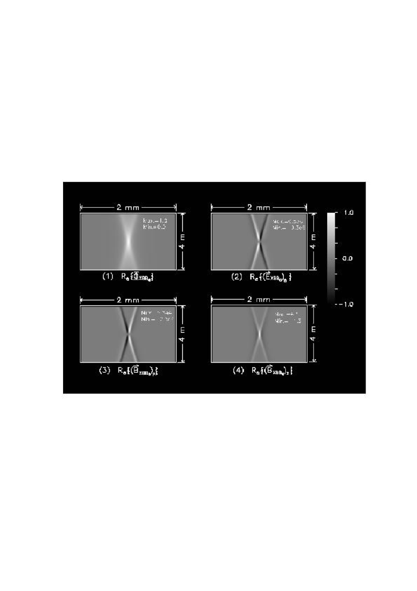
Figure 1: Real part of the Hertz potential and field components of the zeroth-order ($n=0$) localized electromagnetic X-shaped wave at time $t=z/c_{1}$.  Panel (1) is the Hertz potential ${\rm Re}\{\Phi_{X{\rm BB}_{0}}\}$;  Panel (2) is the $\phi$ component of the electric field strength, ${\rm Re}\{(\mbox{\boldmath$E$}_{X{\rm BB}_{0}})_{\phi}\}$;  and Panels (3) and (4) are the $r$ and $z$ components of the magnetic field strength, ${\rm Re}\{(\mbox{\boldmath$H$}_{X{\rm BB}_{0}})_{r}\}$ and ${\rm Re}\{(\mbox{\boldmath$H$}_{X{\rm BB}_{0}})_{z}\}$, respectively.  The dimension of each panel is 4 m ($r$ direction) ${\times}$ 2 mm ($z$ direction). The free parameters $\zeta$ and $a_{0}$ are $0.005^{\rm o}$ and 0.05 mm, respectively. The values shown on the right-top corner of each panel represent the maxima and the minima of the images before normalization for display [MKSA units] (see also Table I).

C. – An Example

In the following, we give an example of electromagnetic X-shaped wave. For simplicity, only the zeroth-order ($n=0$) X-wave is considered. Notice that for $n=0$, eqs.(4’)-(5e) are axially symmetric (not a function of $\phi$), and $(\mbox{\boldmath$E$}_{X{\rm BB}_{0}})_{r}$, $(\mbox{\boldmath$H$}_{X{\rm BB}_{0}})_{\phi}$ and $(\mbox{\boldmath$P$}_{X{\rm BB}_{0}})_{\phi}$ are zero.

The real part of the zeroth-order scalar Hertz potential (eq.(4’)) and the electromagnetic X-shaped waves (eqs.(5b),(5c) and (5e)) are shown in Fig.1. The Poynting flux and energy density are shown in Fig.2. Their maxima and minima are summarized in Tables I and II, respectively. From Table I, we see that, with the parameters given in Fig.1, the electromagnetic X-shaped waves are almost transverse waves where their axial components are much smaller than those of the transverse components. This is also shown in Table II, where the axial component of the Poynting flux is at least four orders larger than its lateral components. Lateral line plots of Figs.1 and 2 along X branches are shown in Fig.3.

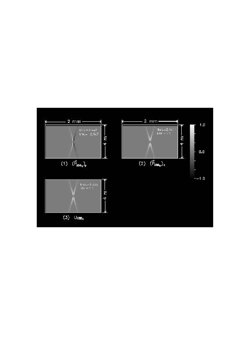
Figure 2: Poynting flux and energy density of the zeroth-order localized electromagnetic X-shaped wave at time $t=z/c_{1}$. Panels (1) and (2) are the $r$ and $z$ components of the Poynting flux, $(\mbox{\boldmath$P$}_{X{\rm BB}_{0}})_{r}$ and $(\mbox{\boldmath$P$}_{X{\rm BB}_{0}})_{z}$, respectively; and Panel (3) is the energy density $U_{X{\rm BB}_{0}}$.  The dimension of each panel and the parameters of the X-waves are the same as those in Fig.1. The values shown on the right-top corner of each panel represent the maxima and the minima of the images before normalizing for display [MKSA units] (see also Table II).

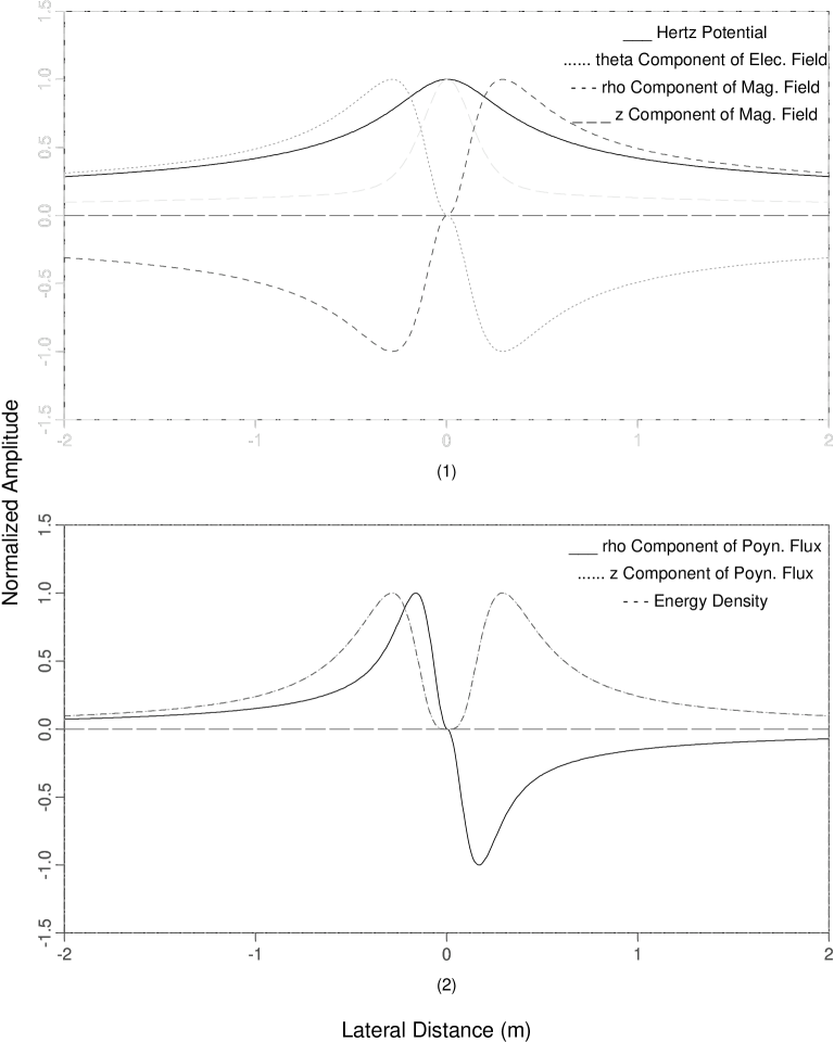
Figure 3: Line plots of the zeroth-order electromagnetic X-shaped wave in Figs.1 and 2 along one of the “X” branches (from left bottom to top right).  Panel (1) shows the line plots of the field components:  ${\rm Re}\{\Phi_{X{\rm BB}_{0}}\}$ (full line);  ${\rm Re}\{(\mbox{\boldmath$E$}_{X{\rm BB}_{0}})_{\phi}\}$ (dotted line);  ${\rm Re}\{(\mbox{\boldmath$H$}_{X{\rm BB}_{0}})_{r}\}$ (dashed line);  ${\rm Re}\{(\mbox{\boldmath$H$}_{X{\rm BB}_{0}})_{z}\}$ (long-dashed line).  Panel (2) is the line plot of the Poynting flux and energy density:  $(\mbox{\boldmath$P$}_{X{\rm BB}_{0}})_{r}$ (full line);  $(\mbox{\boldmath$P$}_{X{\rm BB}_{0}})_{z}$ (dotted line);  and  $U_{X{\rm BB}_{0}}$ (dashed line).

D. – Finite-Aperture Approximation of X-Shaped Waves and their Depth of Field.

The localized electromagnetic X-shaped waves obtained above by us are exact solutions to the free-space Maxwell wave equations. In these equations, there are no boundary conditions and thus the apertures required to produce the waves are infinite; therefore, they cannot be realized in practice. However, these waves can be approximated very well, over a certain “depth of field”, by truncating them in both space and time.

One important question is how far the truncated X-shaped waves can travel without appreciable distortion, i.e., how long is their field depth. The answer is that they travel practically undistorted along a large depth of field, and then they suddenly decay. This has been shown, even experimentally, in the acoustic case[4-6,16,17], and mathematically in the more general case of the slingshot pulses (X-shaped–type waves, found independently in ref.[23] for the case of homogeneous, general scalar wave-equations) as well as for other pulses[15,26].  Let us address the same question in the present (electromagnetic) case.

Since  $|\mbox{\boldmath$E$}_{X{\rm BB}_{n}}(r,\phi,z-c_{1}t)|\ll|\mbox{\boldmath$E$}_{X{\rm BB}_{n}}(r,\phi)|$  and  $|\mbox{\boldmath$H$}_{X{\rm BB}_{n}}(r,\phi,z-c_{1}t)|\ll|\mbox{\boldmath$H$}_{X{\rm BB}_{n}}(r,\phi)|$  for $|z-c_{1}t|>d_{z}/2$  within a finite transverse aperture, where $d_{z}$ is a constant quantity, the X-shaped waves can be truncated e.g. within the axially moving window $[c_{1}t-d_{z}/2,\ c_{1}t+d_{z}/2]$. The truncated waves do not meet the problems of the theoretical (infinitely extended) ones.  If the diameter of the aperture is $D$, the depth of field (which, following Durnin, is defined as the axial distance at which the field amplitude falls to half of that at the surface of the source) of the X-wave Hertz potential (eqs.(4’) and (4”)) is given by[4,16,24,42]

$Z_{\rm max}\ =\ \displaystyle{{D\over 2}\;\displaystyle{{1\over{\sqrt{({c_{1}/c})^{2}-1}}}}}\ =\ \displaystyle{{D\over 2}}\;\cot\zeta\ .$ (8)

Because the derivatives in eqs.(3’) and (3”) do not change the cone angle $\zeta$, the field depth of the electromagnetic X-waves is the same as that of the Hertz potential produced by the same aperture. In addition, eq.(8) is also valid for band-limited electromagnetic X-waves[16].  As an example, if the diameter of the aperture is 20 m and the cone angle is $\zeta=0.005^{\rm o}$, the depth of field of both broadband and band-limited electromagnetic X-waves is 115 km.  For instance, simulation[4] of a finite aperture X-wave Hertz potential with the Rayleigh-Sommerfeld diffraction formula[36] and its production[5] with an acoustic transducer have been reported in the past literature.

Another, even more important question is whether the truncated X-wave (after having been produced, and without further support from the finite antenna) does still travel with Superluminal group-velocity, at least along its depth of field.  One may observe that any wave packet of the type of eq.(4), even with different weights (as far as only $z$ depends on $t$), does not spread in the energy–impulse space;  in other words, there is not spreading in the energy–impulse space of the wave packet even after its truncation, if the linearity between ${{\cal E}}$ and $|\mbox{\boldmath$p$}|$ (i.e., between the coefficients of $z$ and of $t$ in the exponential phase-factor entering eq.(4)) is maintained.  Therefore, after its emission (even if in a truncated form, implying a distortion in the ordinary space, but not in the energy–impulse space), the wave packet’s energetic spectrum does not change, and thus its group velocity $d{{\cal E}}/dk$ is not expected to change too.  We may conclude that, till when the group-velocity has a meaning (i.e., till the abrupt decay of the truncated X-wave), $v_{\rm g}$ is expected to remain Superluminal.

E. – A digression: Localized solutions to the free Schroedinger equation.

We already mentioned that non-diffractive solutions to the quantum equations, including Klein-Gordon’s and Dirac’s, being localized and particle-like, can well be related to elementary particles (and their wave nature)[28,43].  Let us here make a brief digression with respect to the particular case of the Schroedinger equation which, being non-relativistic, presents different problems.

It is well-known[44] that the time-independent Schroedinger and Helmholtz equations are mathematically identical (so that, for instance, the tunnelling of a particle through and under a barrier has been simulated by the travelling of photons in a subcritical waveguide).  Those equations are however different (due to the different order of the time derivative) in the time-dependent case. Nevertheless, it can be shown that they still possess in common classes of analogous solutions, differing only in their spreading properties[45].  We are going to see an example of this fact in the particularly simple case of free space.

The three-dimensional, time-dependent Schroedinger wave equation for free objects is given by

$-\displaystyle{{\hbar\over{2m}}}\;\nabla^{2}\Phi\ =\ i\displaystyle{{{\partial\Phi}\over{\partial t}}}\ ,$

where $\Phi=\Phi(r,\phi,z,t)$ is now the wave-function.  It is easy to verify that eq.(3) is an exact solution also of such equation, if $f(s)=e^{s}$, with  $s=a_{0}(k,\zeta)r\cos(\phi-\theta)+b(k,\zeta)[z-c_{1}(k,\zeta)t]$  and  $c_{1}(k,\zeta)=\hbar[\alpha_{0}^{2}(k,\zeta)+b^{2}(k,\zeta)]/[i2m\,b(k,\zeta)]$.  The quantities $\alpha_{0}(k,\zeta)$ and $b(k,\zeta)$ are any functions of the free parameters $k,\ \zeta$, while $k\equiv 2\pi/\lambda$ it the wave-number and $\lambda$ the wavelength.

Let  $\alpha_{0}(k,\zeta)=-ik\,\sin\zeta$  and  $b(k,\zeta)=ik\,\cos\zeta$;  we then obtain  $c_{1}(k,\zeta)\;=\;\hbar k/[2m\cos\zeta]\;=\;v/[2\cos\zeta]$,  where we used the de Broglie relation $\hbar k=h/\lambda=p$, with $p=mv$, the quantity $v$ being the particle speed.   By using these last relations, and by putting $f(s)=s$,  $T(k)=B(k)\,e^{-a_{0}k}$,  and  $A(\theta)=i^{n}e^{in\theta}$ into eq.(3), we obtain[24] an $n\/$th-order localized solution to the free Schroedinger equation [$n=0,1,2,\ldots$]

$\Phi_{X_{n}}\ =\ e^{in\phi}\;\int_{0}^{\infty}\;B(k)J_{n}(kr\sin\zeta)e^{-k[a_{0}-i\cos\zeta(z-{v\over{2\cos\zeta}}t)]}\;dk\ ,$ (9)

However, in the present non-relativistic case, the integration variable $k$ enters the exponential non-linearly (due to the presence of $v$), so that in eq.(9) the integration cannot be performed in general (a trivial exception being, e.g., the case when the weight $BJ_{n}$ is gaussian).  The same non-linear relation between the coefficients of $z$ and $t$ in the phase factor implies (at variance with the relativistic case) the existence of a spreading.

The group velocity is still given, as usual, by the relation  $\partial[kz\cos\zeta-kvt/2]\,/\,\partial k\;=\;0$, with  $v=\hbar k/m$  But now it is necessary to introduce[46] a mean speed, $\overline{v}$, and only at the price of such an averaging one can write (even in presence of the spreading)  $v_{\rm g}={\overline{v}}/\cos\zeta$.  Quantity $v_{\rm g}$ can be either slower or faster than $v$ (and even than $c$).

If $\zeta=0,\ a_{0}=0$, and $B(k^{\prime})=\delta(k^{\prime}-k)$, eq.(9) represents just a plane wave propagating in the $z$-direction.

For similar work in connection with the Schroedinger equation, see e.g. Barut, refs.[11,28] and Ignatovich[28].  For the relativistic case, see e.g. refs.[47].

IV. – DISCUSSION

A. – Hertz vector potentials and $n\/$th-order X-shaped waves

The scalar X-shaped wave $\Phi_{X{\rm BB}_{n}}$ in eq.(4’) satisfies the wave equation (2). It is the component of a Hertz vector potential in the $z$ direction. If $n=0$, quantity $\Phi_{X{\rm BB}_{0}}$ is axially symmetric and has a single peak at the wave center. For $n>0$, it is zero on the $z$-axis and is axially asymmetric. (When both $n$ and $\zeta$ are zero, $\Phi_{X{\rm BB}_{n}}$ represents the limiting case of a plane wave.)  The Hertz potential $\Phi_{X{\rm BB}_{n}}$, which may or may not have a physical meaning, has been used above as an auxiliary function from which new electromagnetic X-waves are derived, through eqs.(3’) and (3”).  If $\Phi_{X{\rm BB}_{n}}$ is treated approximately as one component of $E$ or of $H$, it has a physical meaning: Many microwave and optical phenomena are treated this way under suitable conditions[36].

From our Hertz vector potential, $\mbox{\boldmath$\Phi$}=\Phi{\hat{\mbox{\boldmath$z$}}}$, the family of electromagnetic X-waves, eqs.(5a)-(5e), has been obtained above, the nonnegative integer $n$ representing the order of the waves. Because the variable $\phi$ appears in $\Phi_{X{\rm BB}_{n}}$ only, $E$ and $H$ have the same axial symmetry as $\Phi_{X{\rm BB}_{n}}$.  However, for $n=1$, $E$ and $H$ are not zero on the axis $z$, and they are not axially symmetric. This means they are not single-valued on the $z$-axis and thus it does not seem they can be approximated with a physical device.

For some components of the electromagnetic X-waves the field on the axial axis $z$ is zero. In such a case, there are multiple peaks around the X-wave center, and the energy density is high on these peaks. For example, the energy density of the zeroth-order electromagnetic X-wave has four sharp peaks (see Panel (3) of Fig.2). This is similar to the case of Ziolkowski’s localized electromagnetic wave[21]. Notice that any higher-order ($n>0$) scalar X-shaped waves are zero on the $z$-axis and also produce multiple peaks[4].

For the electromagnetic X-waves given by eqs.(5a)-(5e),  $(\mbox{\boldmath$E$}_{X{\rm BB}_{n}})_{\phi}/(\mbox{\boldmath$E$}_{X{\rm BB}_{n}})_{r}$  or  $(\mbox{\boldmath$H$}_{X{\rm BB}_{n}})_{\phi}/(\mbox{\boldmath$H$}_{X{\rm BB}_{n}})_{r}$  is not a function of $r$ and $\phi$.  In addition, the $z$-component is very small as compared to the other two components (see Table I). This means that the major component of the Poynting flux (eqs.(6a)-(6c)) is in the $z$ direction (the direction of the vector Hertz potential) (see Table II).

One can make recourse to other Hertz vector potentials, like $\mbox{\boldmath$\Phi$}=\Phi{\hat{\mbox{\boldmath$r$}}}$  or  $\mbox{\boldmath$\Phi$}=\Phi{\hat{\mbox{\boldmath$\phi$}}}$.  In the latter case, by using eq.(4’), we obtain electromagnetic X-waves whose electric components stay in the radial (r,z) plane.  Similarly, in the former case, if $\Phi$ is still an X-wave solution, we obtain localized electromagnetic X-waves with their electric components perpendicular to $\hat{\mbox{\boldmath$r$}}$.  In all these cases, however, for lower-order $\Phi_{X{\rm BB}_{n}}$  (small values of $n$),  $E$ or $H$ may be singular around the axial axis because of terms of the type $1/r$ and $1/r^{2}$.

B. – Method to obtain other limited-diffraction electromagnetic waves

We have seen that, when new localized solutions to eq.(2) are found, the corresponding localized electromagnetic waves can be obtained [cf. for instance eqs.(3’)-(3”)].  There are many ways to obtain new localized solutions to the scalar wave equation, such as the variable substitution method, that converts any existing solutions to a localized solution[48]; and the superposition method, that uses Bessel beams or rather X-waves as basis functions to construct localized beams of practical usefulness[42].

Let us here add the observation that the sidelobes of the scalar X-shaped waves (eq.(4)) are high along the X branches[16]. The asymptotic behaviour of the electromagnetic X-wave sidelobes are similar to that of the scalar waves (see Figs.1 and 2).  Low sidelobes are necessary for example to obtain high contrast imaging. To reduce sidelobes of the scalar X-waves in pulse-echo imaging, recently, unsymmetrical limited diffraction beams such as bowtie X-waves were developed in acoustics[16]: These waves are obtained by taking derivatives in one direction, say $y$, of the zeroth-order X-wave;   when a bowtie X-wave is used to transmit and its $90^{\rm o}$-rotated beam pattern (around the $z$-axis) is used to receive, sidelobes of pulse-echo imaging systems can be reduced dramatically without compromising the image frame rate.  The same technique could also be applied to the electromagnetic X-shaped waves for low sidelobe imaging.

C. – Limited Dispersion and Wave Speed

Because $E$ or $H$ in eqs.(3’)-(3”), and in similar equations are obtained by derivatives of the scalar X-waves in terms of their spatial and time variables, the propagation term $z-c_{1}t$ is retained after the derivatives. Therefore, the electromagnetic X-shaped waves are also localized beams: that is, travelling with the wave at speed $c_{1}$, one will see a constant wave pattern in space.

We have seen that the wave speed $c_{1}$ of localized beams (eq.(1)) along the $z$ axis is greater than or equal to the speed of light (in electromagnetism or optics), or to the speed of sound (in acoustics). For example, the speed of the X-shaped waves is  $c_{1}=c/\cos\zeta\geq c$,  where $0\leq\zeta<\pi/2$ is the cone (Axicon) angle. This behaviour is said to be “tachyonic” or Superluminal[39], and has been studied by many investigators in both “particle”[7,8,49,50] and wave [4-11,23-28,49] physics.  In particular, recently (see e.g. refs.[9,23]) it has been mathematically shown that all relativistic (homogeneous) wave equations admit also sub- and Super-luminal solutions: a claim theoretically confirmed, e.g., in ref.[10] (and that in the past had been verified only in some particular cases[7]).

Although the theoretical Superluminal waves encountered in this paper cannot be exactly produced, due to their infinite energy, they can be approximated with a finite aperture radiator and retain —as we have seen above— their essential characteristics (limited-diffraction and Superluminal group velocity) over a large depth of field. Each component (wavelet) of the approximated wave propagates at the speed of light (or of sound), but the conic, or X-shaped wave, created by their superposition travels at a speed greater than the light (or sound) speed.

The X-waves, however, do not appear to violate[7,39,49] the special theory of relativity, as we are going to discuss below in Section V, when we shall also show that Superluminal X-shaped waves, in particular, are predicted by Relativity itself to travel in space rigidly, without deforming[7,39].

Since Superluminal motions seem to appear even in other sectors of experimental science, we deem it proper to present in an Appendix at the end of this paper some information about those experimental results. In fact, the subject of Superluminal objects [or tachyons] addressed in this paper is still regarded frequently as unconventional, and in this respect it can get therefore more support from experiments than from theory.  Moreover, such pieces of information are presently scattered in four different areas of science, and it can be useful to find them all collected in one and the same place.

D. – Role of superposition and interference

The X-waves considered by us are a superposition of Bessel beams and therefore can be regarded, eventually, as linear superposition of $c$-speed plane waves travelling at different angles about the beam axis. If the aperture is infinite, plane waves will not deform and diverge as they propagate to infinity.  If the aperture is finite, plane waves travel to a large distance in which they do not diverge significantly: However, beyond that large distance, plane waves, so the X-waves, start to diverge.  The speed of the X-waves along the axis, that is greater than $c$, is caused by the plane waves that do not travel along the axis but at an angle (Axicon angle) with it.

If the aperture is infinite, X-waves travel to infinite distance without deformation: This is because antennas continue to support the waves from the X branches which extend to infinity in time as the aperture goes to infinity (remember that the X-wave extension in time is equal to $(D/2)\,\tan\zeta$, where $D$ is the diameter of the aperture and $\zeta$ is the cone angle).

If the X-waves are truncated, they are no longer X-waves in the original sense. As soon as truncated X-waves leave the source that produces them, they start deforming progressively. We have seen that the truncated X-waves deforms negligibly within their depth of field and significantly beyond it; the peak of the truncated X-waves happens near the wave axis: it travels faster than $c$. Beyond the support (depth of field) of the X branches, truncated waves start to diverge quickly. In the limit (infinite distance), truncated X-waves behave like a spherical wave travelling at speed $c$. In conclusion, truncated X-waves can send signals at a speed greater than $c$ only within the support of the X branches: but this is achieved at the cost that the wave front must be leaning forward in space to form the advanced X branches.  Namely, the outmost ring of the finite antenna has to be excited first; then, since the waves from this ring travel at $c$, the peak of the X-waves travels faster than $c$ on the axis.  The waves deform quite dramatically near the boundary of the depth of field $d=a\cot\zeta$, where $a$ is the radius of the circular aperture and $\zeta$ is the cone angle.

Notice that, however, the peak (vertex) of the truncated X-wave is formed with wave components from the X branches in a continuously changing way as the beam propagates, so that it does not represent the speed of the centroid of the beam.  This is particularly true when the arms carry large amounts of energy.

V. – A THEORETICAL FRAMEWORK WITHIN SPECIAL RELATIVITY FOR THE X-SHAPED WAVES

Let us here mention that a simple theoretical framework exists[7] (merely based on the space-time geometrical methods of Special Relativity (SR)) which incorporates the Superluminal X-shaped waves without violating the Relativity principles.

Actually, SR can be derived from postulating: (i) the Principle of relativity; and (ii) space-time to be homogeneous and space isotropic.  It follows that one and only one invariant speed exists; and experience shows that invariant speed to be the one, $c$, of light in vacuum (the essential role of $c$ in SR being just due to its invariance, and not to its being supposedly a maximal, or minimal, speed; no other, sub- or Super-luminal, object can be endowed with an invariant speed: in other words, no bradyon or tachyon can play in SR the same essential role as the speed-$c$ light waves). Let us recall, incidentally, that tachyon [a term coined in 1967 by G.Feinberg] and bradyon [a term coined in 1970 by E.Recami] mean Superluminal and subluminal object, respectively. The speed $c$ turns out to be a limiting speed: but any limit possesses two sides, and can be approached a priori both from below and from above.  (As E.C.G.Sudarshan put it, from the fact that no one could climb over the Himalayas ranges, people of India cannot conclude that there are no people North of the Himalayas…; actually, speed-$c$ photons exist, which are born, live and die just “at the top of the mountain,” without any need to accelerate from rest to the light speed).

A consequence is that the quadratic form  $ds^{2}=c^{2}dt^{2}-dx^{2}-dy^{2}-dz^{2}$  (i.e., the four-dimensional length-element square, along the space-time path of any object) results to be invariant, except for its sign.  In correspondence with the positive (negative) sign, one gets the subluminal (Superluminal) Lorentz transformations [LT]. The ordinary, subluminal LTs leave, e.g., the fourvector squares and the scalar products (between fourvectors) just invariant.

The Superluminal LTs can be easily written down only in two dimensions (or in six, or in eight, dimensions…). But they must have the properties of changing sign, e.g., to the fourvector squares and to the fourvector scalar products. This is enough to deduce —see Fig.4— that a particle, which is spherical when at rest (and which appears then as ellipsoidal, due to Lorentz contraction, at subluminal speeds $v$), will appear[7,39,40,51] as occupying the cylindrically symmetrical region bounded by a two-sheeted rotation hyperboloid and an indefinite double cone, as in Fig.4(d), for Superluminal speeds $V$. In Fig.4 the motion is along the $x$-axis. In the limiting case of a point-like particle, one obtains only a double cone. In 1980-1982, therefore, it was predicted[39] that the simplest Superluminal object appears (not as a particle, but as a field or rather) as a wave: namely, as a “X-shaped wave”, the cone semi-angle $\alpha$ being given (with $c=1$) by  $\cot\alpha=\sqrt{V^{2}-1}$.

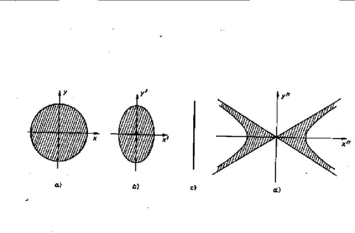
Figure 4: Let us consider an object that is intrinsically spherical, i.e., that is a sphere in its rest-frame (Panel (a)). After a generic subluminal Lorentz transformation (LT) along $x$, i.e., under a subluminal $x$-boost, it is predicted by special relativity (SR) to appear as ellipsoidal due to Lorentz contraction (Panel (b)). After a Superluminal $x$-boost (namely, when this object moves with Superluminal speed $V$), it is predicted by extended relativity (ER) to appear[7,39] as in Panel (d), i.e., as occupying the cylindrically symmetric region bounded by a two-sheeted rotation hyperboloid and an indefinite double cone. The whole structure is predicted by ER to move rigidly[39] and, of course, with the speed $V$, the cotangent square of the cone semi-angle being $(V/c)^{2}-1$.  Panel (c) refers to the limiting case when the boost-speed tends to $c$, either from the left or from the right. (For simplicity, a space axis is skipped).

It was also predicted[39,51] that the X-shaped waves would move rigidly with speed $V$ along their motion direction (Fig.5). The reason for such “X-waves” to travel without deformation is quite simple: every X-wave can be regarded at each instant of time as the (Superluminal) Lorentz transform of a spherical object, which of course as time elapses moves in vacuum without any deformation.

The X-shaped waves here considered are the most simple ones only. If we started not from an intrinsically spherical or point-like object, but from a non-spherically symmetric particle, or from a pulsating (contracting and dilating) sphere, or from a particle oscillating back and forth along the motion direction, their Superluminal Lorentz transforms would result to be more and more complicated. The above-seen X-waves, however, are typical for a Superluminal object, so as the spherical or point-like shape is typical for a subluminal particle.

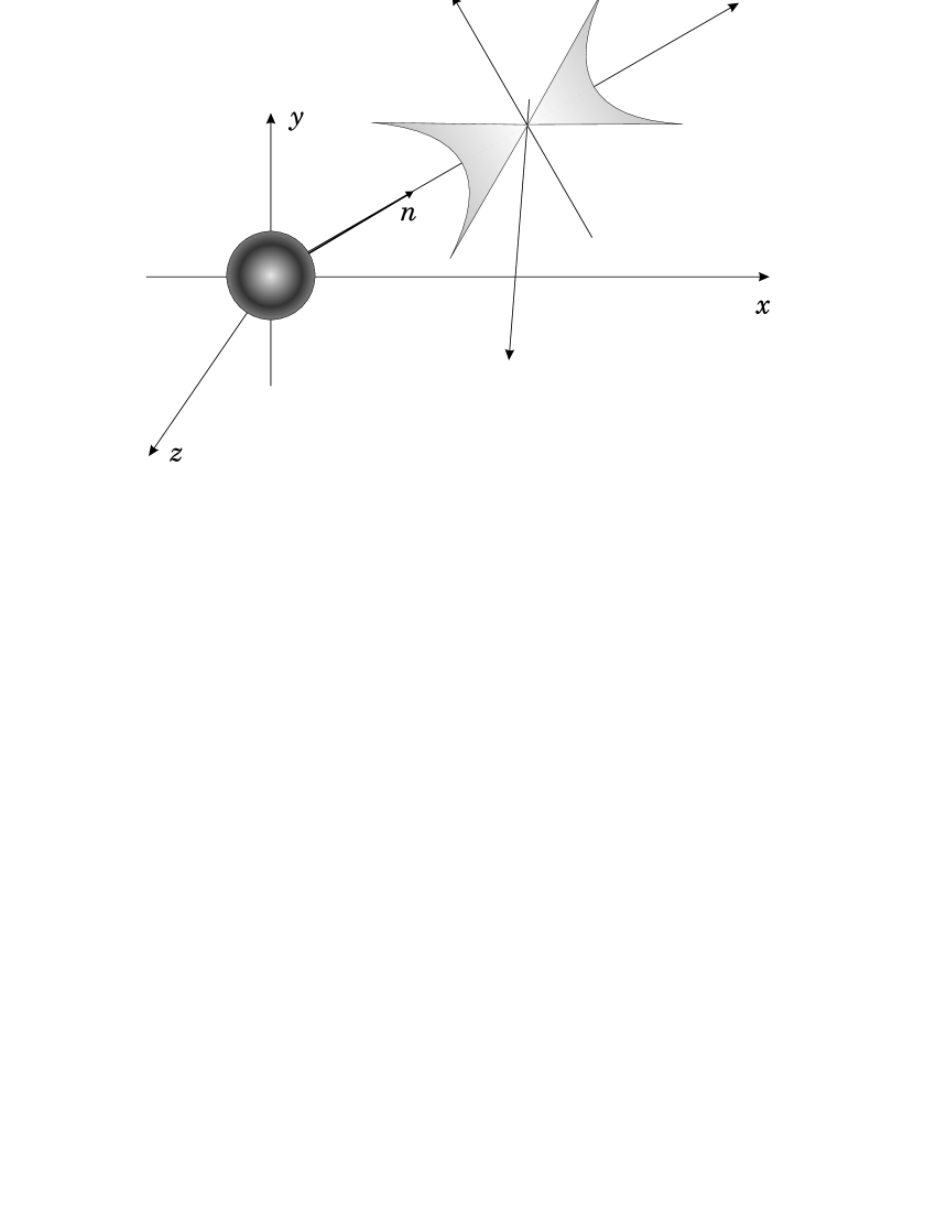
Figure 5: If we start from a spherical particle as in Fig.4(a), then —after a Superluminal boost along a generic motion line $l$— we obtain the tachyonic object $T$ depicted in this figure.  Once more, the Superluminal object $T$ appears to be spread over the whole spatial region delimited by a double cone and a two-sheeted hyperboloid asymptotic to the cone[51]. The whole structure travels of course along $l$ with the speed $V$ of the Superluminal $l$-boost.  Notice that, if the object is not spherical when at rest (but, e.g., is ellipsoidal in its own rest-frame), then the axis of $T$ will no longer coincide with $l$, but its direction will depend on the speed $V$ of the tachyon itself.  For the case in which the space extension of the Superluminal object $T$ is finite, see ref.[40].

The three dimensional picture of Fig.5, or rather of Fig.4(d), appears in Fig.6, where its annular intersections with a transverse plane are shown (cf. refs.[39,51]).

It has been believed for a long time that Superluminal objects would have allowed sending information into the past; but such problems with causality seem to be solvable within SR. Once SR is generalized in order to include tachyons, no signal travelling backwards in time is apparently left. For a solution of those causal paradoxes, see refs.[49,50] and references therein.

Let us pass, within this elementary context, to the problem of producing a “X-shaped wave” like the one depicted in Fig.6 (truncated of course, in space and in time, by use of a finite antenna radiating for a finite time interval). To convince ourselves about the possibility of realizing them, it is enough to consider naïvely the ideal case of a Superluminal source S of negligible size, endowed with constant speed $V$ and emitting spherical electromagnetic waves $W$ (each one travelling at the invariant speed $c$). We shall observe the electromagnetic waves to be internally tangent to an enveloping cone C having the source motion line $x$ as its axis and $S$ as its vertex. This is analogous to what happens with an airplane moving with a constant supersonic speed in the air.  In addition, those electromagnetic waves W interfere negatively one another inside the cone C, and interfere constructively only on its surface. We can put a plane detector orthogonal to $x$ and record the intensity and direction of the waves W impinging on it, as a (cylindrically symmetric) function of position and of time. Afterwards, it will be enough to replace the plane detector by a plane antenna that radiates —instead of detecting and recording— exactly the same (cylindrically symmetrical) space-time pattern of electromagnetic waves W, in order to build up a cone-shaped (C) electromagnetic wave travelling along $x$ with the Superluminal speed $V$ (obviously, with no radiating source any longer —now— at its vertex S). Even if each spherical wave W will still travel with the invariant speed $c$.

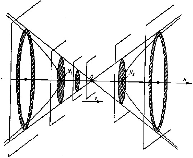
Figure 6: Here we show the intersections of the Superluminal object $T$ with planes $P$ orthogonal to its motion line (the $x$-axis) for the same case as in Fig.4.  For simplicity, we assumed again the object to be spherical in its rest-frame, and the cone vertex to coincide with the origin O for $t=0$.  Such intersections evolve in time so that the same pattern appears on a second plane —shifted by $\Delta x$ after the time $\Delta t=\Delta x/V$.  On each plane, as time elapses, the intersection is therefore predicted by ER to be a circular ring which, for negative times, goes on shrinking until it reduces to a circle and then to a point (for $t=0$);  afterwards, such a point becomes again a circle and then a circular ring that goes on broadening[7,39,40,51.

Incidentally, the above-mentioned evaluation can lead to a very simple type of “X-shaped wave.”

These examples are to be completed, however, by recalling that Special Relativity implies considering also the forward cone: cf. Fig.6.  The truncated X-waves considered in this paper, for instance, must have a leading cone in addition to the rear cone; such a leading cone having an essential role for the peak travelling faster than $c$.  In other words, in the approximated case in which we produce a finite conic wave truncated both in space and in time, the theory of SR suggested the bi-conic shape (symmetrical in space with respect to the vertex S) to be a priori a better approximation to a rigidly travelling wave; so that SR suggests to have recourse to an antenna emitting a radiation (not only cylindrically symmetrical in space but also) symmetric in time, for a better approximation to an undistorted progressive wave.

Let us recall once more that our truncated (finite) bi-conic, or X-shaped, waves (after having been produced) are expected to travel almost rigidly, at Superluminal speed, all along their depth of field (but only along such depth of field).

One may observe, at last, that in the vacuum and in homogeneous media for the (non truncated) X-shaped waves the group velocity coincides with the phase velocity.

VI. – CONCLUSION

We have derived and considered various localized X-shaped solutions to the free Maxwell equations, which possess Superluminal group velocities. Theoretically, these solutions are diffraction-free. They are infinitely extended in space and time, and —the ones met in this work— possess infinite total energy. However, for solutions that are single valued and non-singular (finite energy density), they can be approximated very well by a finite aperture antenna over a large depth of interest (along which the truncated X-shaped waves maintain their essential characteristics of limited-diffraction and Superluminal velocity).  In addition, localized, limited-diffraction wave solutions to the quantum equations can be helpful for a better understanding of the relationship between waves and particles.  Because (practically realizable) localized beams have a large depth of field, they have and can have applications in several areas, from electromagnetism, communications and optics to acoustics and geophysics.

As explained in Sect.IV–C above, we use the present occasion to present in the Appendix below some information about the other sectors of experimental science in which Superluminal motions seem to appear.

VII. – ACKNOWLEDGMENTS

We gratefully acknowledge that this paper is based on work developed in collaboration with Professors Dr. Jian-yu Lu and Dr. J.F.Greenleaf and appeared in preliminary form as Report INFN/FM–96/01 (I.N.F.N.; Frascati, 1996)  [its number in the electronic LANL Archives being # physics/9610012;  Oct.15, 1996]; in particular, the Tables and Figs.1–3 are due to Lu and Greenleaf.   The mistakes eventually appearing in this article, however, are the responsibility of the present author only.  The first three figures of that Report, and of this paper, will be used —by permission of Lu, Greenleaf and Recami— also in a paper by W.A.Rodrigues Jr. and J.-y.Lu (submitted to Found. Phys.).  The author is very grateful to the co-editor, Prof.D.Stauffer, for many helpful critical comments.  He appreciates for useful discussions, moreover, Dr. Vladislav S. Olkhovsky, of the Institute for Nuclear Physics of the Ukrainian Academy of Sciences, Kiev; Dr. Amr M. Shaarawi, of the Faculty of Engineering, Cairo University, Giza, Egypt; Dr. Peeter Saari, of the Tartu University, Estonia; and Dr. Hugo E. Hernández and Dr. L. C. Kretly, of the D.M.O.-FEEC and of the C.C.S., respectively, at the Universidade Estadual de Campinas, Campinas, S.P., Brazil.

VIII. – APPENDIX

In this Appendix we take the opportunity to present some sketchy information —mainly bibliographical— about the other three (in total, four) sectors of experimental science in which Superluminal motions seem to appear. In fact, as the “Superluminal” topic is still controversial, a panoramic view of the overall experimental situation is certainly useful, especially when it is considered that the related information, scattered in very different Journals, is not all of easy access to everybody.

The question of Superluminal objects or waves [tachyons] has a long story, starting perhaps with Lucretius’ De Rerum Natura. Still in pre-relativistic times, let us recall e.g. the contributions by A.Sommerfeld. In relativistic times, our problem started to be tackled again essentially in the fifties and sixties, in particular after the papers by E.C.George Sudarshan et al., and later on by E.Recami, R.Mignani et al. [who by their numerous works at the beginning of the seventies rendered, by the way, the terms sub- and Super-luminal of popular use], as well as by H.C.Corben and others (to confine ourselves to the theoretical researches). For references, one can check pages 162-178 in ref.[7], where about 600 citations are listed; or the large bibliographies by V.F.Perepelitsa[52] and the book in ref.[53]. In particular, for the causality problems one can see refs.[49,50] and references therein, while for a model theory for tachyons in two dimensions one can be addressed to refs.[7,8]. The first experiments looking for tachyons were performed by T.Alvager et al.; some citations about the early experimental quest for Superluminal objects being found e.g. in refs.[7,54].

The subject of tachyons is presently returning after fashion, especially because of the fact that four different experimental sectors of physics seem to indicate the existence of Superluminal objects; including —of course— the one dealt with in this and in other papers of ours: which appears to us as being at the moment the most important sector. Let us put forth in the following some brief information about the experimental results obtained in such different science areas.

1. – Negative square-mass neutrinos

Since 1971 it was known that the experimental square-mass of muon-neutrinos resulted to be negative[55]. If confirmed, this would correspond (within the ordinary naive approach to relativistic particles) to an imaginary mass and therefore to a Superluminal speed. [In a non-naive approach[7], i.e. within a Special Relativity theory extended to include tachyons (Extended Relativity), the free tachyon “diffraction relation” (with $c=1$) becomes actually  $E^{2}-\mbox{\boldmath$p$}^{2}=-m_{0}^{2}$, so that one does not have to associate tachyons with imaginary-mass particles!].

From the theoretical point of view, let us refer to [56] and references therein.

It is rather important that recent experiments showed that also electron-neutrinos have negative mass-square[57].

2. – Galactic “Mini-Quasars”

We refer ourselves to the apparent Superluminal expansions observed inside quasars, some galaxies, and —as discovered very recently— in some galactic objects, preliminarily called “mini-quasars”. Since 1971 in many quasars apparent Superluminal expansions were observed [Nature, for instance, dedicated a cover of its to those observations on 2 Apr.1981]. Such seemingly Superluminal expansions were the consequence of the experimentally measured angular separation rates, once it was taken account of the (large) distance of the sources from the Earth. From the experimental point of view, it will be enough to quote the book [58] and references therein.

The distance of those “Superluminal sources”, however, is not well-known; or, at least, the (large) distances usually adopted have been strongly criticized by H.Arp et al., who maintain that quasars are much nearer objects than expected: so that all the above-mentioned data can no longer be easily used to infer (apparent) Superluminal motions. However, very recently, galactic objects have been discovered, in which apparent Superluminal expansions occur; and the distance of the galactic objects can be more precisely determined. For the experimental data, see refs.[59].

For a theoretical point of view, both for quasars and “mini-quasars”, see refs.[7,60]. In particular, let us recall that a single Superluminal source of light would just be observed: (i) initially, in the phase of “optic boom” (analogous to the acoustic “boom” by an aircraft that travels with constant super-sonic speed) as a suddenly-appearing intense source; (ii) later on, as a source which splits into TWO objects receding one from the other with relative velocity V larger than 2c.

3. – Tunnelling photons = Evanescent waves

It is the sector that most attracted the attention of the scientific and non-scientific press[61].

Evanescent waves were predicted [cf., e.g., ref.[7], page 158 and references therein] to be faster-than-light. Even more, they consist in tunnelling photons: and it was known since long time[62] that tunnelling particles (wave packets) can move with Superluminal group–velocities inside the barrier; therefore, due to the theoretical analogies between tunnelling particles (e.g., electrons) and tunnelling photons[44], it was since long expected that evanescent waves could be Superluminal.

The first experiments have been performed in Cologne, Germany, by Guenter Nimtz et al., and published in 1992. See refs.[63].

Important experiments have been performed in Berkeley: see refs.[64].

Further experiments on Superluminal evanescent waves have been done in Florence[65]; while a last experiment (as far as we know) took place in Vienna[66].

From the theoretical point of view, see refs.[62] and references therein; and refs.[67].

4. – Superluminal motions in Electrical and Acoustical Engineering — The “X-shaped waves”

This fourth sector, which this paper is contributing to, seems to be at the moment (together with the third one) the most promising.

Starting with the pioneering work by H.Bateman, it became slowly known that all the relativistic homogeneous wave equations —in a general sense: scalar, electromagnetic and spinorial— admit solutions with subluminal group velocities[1]. More recently, also Superluminal solutions have been constructed for those homogeneous wave equations, in refs.[2,10] and quite independently in refs.[6,9,23]: in some cases just by applying a Superluminal Lorentz “transformation”[7,8]. It has been shown that an analogous situation is met even for acoustic waves, with the existence in this case of “sub-sonic” and “Super-sonic” solutions[3,4];  so that one can expect they to exist, e.g., also for seismic wave equations. (More intriguingly, one might expect the same to be true in the case of gravitational waves too).

Let us recall that the rigidly travelling Supersonic and Superluminal solutions found in refs.[4,5,23,27] and in this paper —some of them already experimentally realized— appear to be (generally speaking) X-shaped, just as predicted in 1980/1982 by Barut, Recami and Maccarrone[39].

On this regard, from the theoretical point of view, let us quote pages 116-117, and pages 59 (fig.19) and 141 (fig.42), of ref.[7]; and even more refs.[7,40,51], where “X-type waves” are predicted and discussed. From such papers it results also clear why the X-shaped waves keep their form while travelling (non-diffractive waves).

Note added: during the about two years elapsed between original submission and publication, many relevant papers appeared in print. Quotations of various of them have been directly included in the References. After the revision of the citations, however, some further important articles appeared. Let us mention in particular that:  (i) at Tartu (Estonia) they have experimentally produced X-shaped (Superluminal) light waves, in optics: see P.Saari and K.Reivelt: “Evidence of X-shaped propagation-invariant localized light waves”, appeared in Phys. Rev. Lett., Nov.24, 1997;  H.Sõnajalg, M.Rätsep and P. Saari: Opt. Lett. 22 (1997) 310; and P.Saari and H.Sõnajalg: Laser Phys. 7 (1997) 32;  (ii) simultaneously, (non-truncated) X-shaped beams with finite total energy —expected to exist on the basis of ER— were mathematically constructed by I.Besieris, M.Abdel-Rahman, A.Shaarawi and A.Chatzipetros in the work “Two fundamental representations of localized pulse solutions to the scalar wave equation”, to appear in J. Electromagnetic Waves Appl. (1998).

References

[1] H.Bateman: Electrical and Optical Wave Motion (Cambridge Univ.Press; Cambridge, 1915);  A.O.Barut and A.Grant: Found. Phys. Lett. 3 (1990) 303; A.O.Barut and A.J.Bracken: Found. Phys. 22 (1992) 1267.  See also refs.[14,19,20] below.

[2] A.O.Barut and H.C.Chandola: Phys. Lett. A180 (1993) 5. See also A.O.Barut: Phys. Lett. A189 (1994) 277-280, and A.O.Barut et al.: refs.[1].

[3] Jian-yu Lu and J.F.Greenleaf: IEEE Transactions on Ultrasonics, Ferroelectrics, and Frequency Control 37 (1990) 438-447.

[4] Jian-yu Lu and J.F.Greenleaf: IEEE Transactions on Ultrasonics, Ferroelectrics, and Frequency Control 39 (1992) 19-31 (awarded paper).  Cf. also ref.[23], where X-shaped–type waves were found and called “slingshot pulses”.

[5] Jian-yu Lu and J.F.Greenleaf: IEEE Transactions on Ultrasonics, Ferroelectrics, and Frequency Control 39 (1992) 441-446 (awarded paper).

[6] R.Donnelly, D.Power, G.Templeman and A.Whalen: IEEE Transactions on Ultrasonics, Ferroelectrics and Frequency Control 41 (1994) 7-12.

[7] E.Recami: “Classical tachyons and possible applications,” Rivista Nuovo Cimento 9 (1986), issue no.6, pp.1-178; and refs. therein.

[8] E.Recami and W.A.Rodrigues: “A model theory for tachyons in two dimensions”, in Gravitational Radiation and Relativity, J.Weber and T.M.Karade editors (World Scient.; Singapore, 1985), pp.151-203.

[9] See e.g. R.Donnelly and R.W.Ziolkowski: Proc. Royal Soc. London A440 (1993) 541.  Cf. also I.M.Besieris, A.M.Shaarawi and R.W.Ziolkowski: J. Math. Phys. 30 (1989) 1254-1269.

[10] S.Esposito: Phys. Lett. A225 (1997) 203;  W.A.Rodrigues Jr. and J.Vaz Jr., “Subluminal and superluminal solutions in vacuum of the Maxwell equations and the massless Dirac equation,” to appear in Adv. Appl. Cliff. Alg.

[11] R.W.Ziolkowski: Phys. Rev. A39 (1989) 2005-2033;  A44 (1991) 3960-3984;  R.W.Ziolkowski, D.K.Lewis and B.D.Cook: Phys. Rev. Lett. 62 (1989) 147-150;  R.W.Ziolkowski, I.M.Besieris and A.M.Shaarawi: Proceed. IEEE 79 (1991) 1371-1378;  A.M.Shaarawi, I.M.Besieris and R.W.Ziolkowski: Optics Comm. 116 (1995) 183-192;  G.Indebetouw: J. Opt. Soc. Am. 6 (1989) 150-152;  P.L.Overfelt: Phys. Rev. A44 (1991) 3941;  A.O.Barut: Phys. Lett. A143 (1990) 349;  A.O.Barut and A.Grant: in ref.[1];  A.O.Barut: in L. de Broglie, Heisenberg’s Uncertainties and the Probabilistic Interpretation of Wave Mechanics (Kluwer; Dordrecht, 1990);  A.O.Barut: “Quantum theory of single events: Localized de Broglie–wavelets, Schroedinger waves and classical trajectories”, preprint IC/90/99 (ICTP; Trieste, 1990).

[12] R.Courant and D.Hilbert: Methods of Mathematical Physics (J.Wiley; New York, 1966), vol.2, p.760.

[13] J.A.Stratton: Electromagnetic Theory (McGraw-Hill; New York, 1941), p.356.

[14] J.Durnin: J. Opt. Soc. Am. 4 (1987) 651-654;  J.Durnin, J.J.Miceli Jr. and J.H.Eberly: Phys. Rev. Lett. 58 (1987) 1499-1501;  Opt. Lett. 13 (1988) 79.  See also P.Saari and H.Sõnajalg: quoted in the Note added in proofs.

[15] See e.g. A.M.Vengsarkar, I.M.Besieris, A.M.Shaarawi and R.W.Ziolkowski: J. Opt. Soc. Am. A9 (1992) 937-949;  S.M.Sedky, A.M.Shaarawi, I.M.Besieris and F.M.M.Taiel: J. Opt. Soc. Am. A13 (1996) 1719-1727;  R.W.Ziolkowski and D.K.Lewis: J. Appl. Phys. 68 (1990) 6083;  R.W.Ziolkowski, I.M.Besieris and A.M.Shaarawi: in ref.[11];  A.M.Shaarawi, I.M.Besieris and R.W.Ziolkowski: J. Appl. Phys. 65 (1989) 805-813.  See also B.Salik, J.Rosen and A.Yariv: Opt. Lett. 20 (1995) 1743.

[16] Jian-yu Lu: IEEE Transactions on Ultrasonics, Ferroelectrics and Frequency Control 42 (1995) 1050-1063;  40 (1993) 735-746.

[17] Jian-yu Lu, He-hong Zou and J.F.Greenleaf: Ultrasound in Medicine and Biology 20 (1994) 403-428.

[18] Jian-yu Lu and J.F.Greenleaf: Ultrasonic Imaging 15 (1993) 134-149.

[19] J.N.Brittingham: J. Appl. Phys. 54 (1983) 1179-1189.

[20] R.W.Ziolkowski: J. Math. Phys. 26 (1985) 861-863.  Cf. also R.W.Ziolkowski, D.K.Lewis and B.D.Cook: in ref.[11].

[21] R.W.Ziolkowski: refs.[11].

[22] K.Uehara and H.Kikuchi: Appl. Physics B48 (1989) 125-129;  J.Rosen, B.Salik, A.Yariv and H.-K. Liu: Opt. Lett. 20 (1995) 423;  D.Eliyahu, R.A.Salvatore, J.Rosen, A.Yariv and J.-J.Drolet: Opt. Lett. 20 (1995) 1412.

[23] R.W.Ziolkowski, I.M.Besieris and A.M.Shaarawi: J. Opt. Soc. Am. A10 (1993) 75.  Cf. also R.W.Ziolkowski: in ref.[11].

[24] J.-y.Lu, J.F.Greenleaf and E.Recami: “Limited-diffraction solutions to Maxwell (and Schroedinger) equations”, Report INFN/FM–96/01 (INFN; Frascati, 23 Oct.1996); electronic LANL Archives # physics/9610012;  Oct.15, 1996.

[25] Hugo Hernández F.,  A.Pablo L.Barbero and  E.Recami: (unpublished).

[26] A.M.Vengsarkar, I.M.Besieris, A.M.Shaarawi and R.W.Ziolkowski: in ref.[15].  See also I.M.Besieris, A.M.Shaarawi and R.W.Ziolkowski: in ref.[9];  A.M.Shaarawi, I.M.Besieris and R.W.Ziolkowski: J. Math. Phys. 31 (1990) 2511-2519;  J.Fagerholm, A.T.Friberg, J.Huttunen, D.P.Morgan and M.M.Salomaa: Phys. Rev. E54 (1996) 4347-4352.

[27] H.Sõnajalg and P.Saari: Opt. Lett. 21 (1996) 1162-1164;  P.Saari: in Ultrafast Processes in Spectroscopy, ed. by A.Svelto et al. (Plenum; New York, 1996), pp.151-156.  Cf. also J.Turunen, A.Vasara and A.T.Friberg: J. Opt. Soc. Am. A8 (1991) 282;  K.Reivelt: Thesis (Univ. of Tartu; 1995).

[28] A.M.Shaarawi, I.M.Besieris and R.W.Ziolkowski: in ref.[26], especially Sect.VI;  Nucl Phys. (Proc.Suppl.) B6 (1989) 255-258;  Phys. Lett. A188 (1994) 218-224;  A.O.Barut: Phys. Lett. A171 (1992) 1-2;  Ann. Foundation L. de Broglie, Jan.1994;  and the last one of refs.[11].  See also V.K.Ignatovich: Found. Phys. 8 (1978) 565-571;  A.Garuccio and V.A.Rapisarda: Nuovo Cimento A65 (1981) 269-297;  D.Bambusi et al.: “On the relevance of classical electrodynamics for the foundations of Physics”, Milano Univ. preprint (Dip.Mat,; Milan, 1997?).

[29] Jian-yu Lu: “Producing bowtie limited diffraction beams with synthetic array experiment,” IEEE Transactions on Ultrasonics, Ferroelectrics, and Frequency Control (in press), and refs. therein;  “Limited diffraction array beams,” International Journal of Imaging System and Technology (in press), and refs. therein.

[30] D.K.Hsu, F.J.Margetan and D.O.Thompson: Appl. Phys. Lett. 55 (1989) 2066-2068;  J.A.Campbell and S.Soloway: J. Acoust. Soc. Am. 88 (1990) 2467-2477.

[31] Jian-yu Lu and J.F.Greenleaf: in IEEE Ultrasonics Symposium Proceedings (91CH3079-1), vol.2 (1991) pp.1155-1159.

[32] Tai K.Song, Jian-yu Lu and J.F.Greenleaf: Ultrasonic Imaging 15 (1993) 36-47.

[33] Jian-yu Lu and J.F.Greenleaf: Ultrasound in Medicine and Biology 17 (1991) 265-281.

[34] G.S.Kino: Acoustic Waves: Device, Imaging, and Analog Signal Processing (Prentice-Hall; Englewood Cliffs, NJ, 1987), chapts.2 and 3.

[35] E.Heyman, B.Z.Steinberg and L.B.Felsen: J. Opt. Soc. Am. A4 (1987) 2081-2091.

[36] J.W.Goodman: Introduction to Fourier Optics (McGraw-Hill; New York, 1968), chapts.2-4.  See also G. Toraldo di Francia: Onde Elettromagnetiche (Zanichelli; Bologna, 1988).

[37] J.H.McLeod: J. Opt. Soc. Am. 44 (1954) 592.

[38] E.P.Wigner: Phys. Rev. 98 (1955) 145.

[39] A.O.Barut, G. D.Maccarrone and E.Recami, “On the shape of tachyons,” Nuovo Cimento A71 (1982) 509-533.  See also E.Recami and G.D.Maccarrone: Lett. Nuovo Cim. 28 (1980) 151-157;  P.Caldirola, G.D.Maccarrone and E.Recami: Lett. Nuovo Cim. 29 (1980) 241-250.

[40] E.Recami and G.D.Maccarrone: Lett. Nuovo Cimento 37 (1983) 345-352.

[41] Cf., e.g., V.A.Rapisarda: Lett. Nuovo Cim. 33 (1982) 437-444;  F.Falciglia, A.Garuccio and L.Pappalardo: Lett. Nuovo Cim. 34 (1982) 1, and refs. therein.

[42] Jian-yu Lu: in IEEE 1995 Ultrasonic Symp. Proceed. (95CH35844), vol.2 (1995) pp.1393-1397;  “Designing limited diffraction beams”, in IEEE Transactions on Ultrasonics, Ferroelectrics and Frequency Control (in press).

[43] Cf. e.g. A.O.Barut: Phys. Lett. A143 (1990) 349;  Found. Phys. 20 (1990) 1233;  P.Hillion: Phys. Lett. A172 (1992) 1;  A.M.Shaarawi, I.M.Besieris and R.W.Ziolkowski: in ref.[26];  in ref.[28];  and  Nuclear Physics (Proc.Suppl.) B6 (1989) 255.

[44] See, e.g., Th.Martin and R.Landauer: Phys. Rev. A45 (1992) 2611;  R.Y.Chiao, P.G.Kwiat and A.M.Steinberg: Physica B175 (1991) 257;  A.Ranfagni, D.Mugnai, P.Fabeni and G.P.Pazzi: Appl. Phys. Lett. 58 (1991) 774.  See also A.M.Steinberg: Phys. Rev. A52 (1995) 32.

[45] A.Agresti, V.S.Olkhovsky and E.Recami: (to be submitted for pub.)

[46] M.L.Goldberger and K.M.Watson: Collision Theory (Wiley; New York, 1963).

[47] A.M.Shaarawi, I.M.Besieris and R.W.Ziolkowski: in ref.[26], and refs. therein;  and  in ref.[28].

[48] Jian-yu Lu, He-hong Zou and J.F.Greenleaf: IEEE Transactions on Ultrasonics, Ferroelectrics and Frequency Control 42 (1995) 850-853.  See also A.T.Friberg, J.Fagerholm and M.M.Salomaa: Opt. Comm. 136 (1997) 207-212.

[49] E.Recami: “Tachyon kinematics and causality”, Foundation of Physics 17 (1987) 239-296.

[50] E.Recami: “The Tolman ‘Anti-telephone’ paradox: Its solution by tachyon mechanics,” Lett. Nuovo Cimento 44 (1985) 587-593.

[51] G.D.Maccarrone, M.Pavsic and E.Recami: Nuovo Cimento B73 (1983) 91-111.

[52] V.F.Perepelitsa: Reports ITEF-100 and ITEF-165 (Institute of Theoretical and Experimental Physics; Moscow, 1980).

[53] E.Recami (editor): Tachyons, Monopoles, and Related Topics (North-Holland; Amsterdam, 1978).

[54] See e.g. D.F.Bartlett et al.: Phys. Rev. D18 (1978) 2253; P.N.Bhat et al.: J. Phys. G5 (1979) L13.  Cf. also A.S.Goldhaber and F.Smith: Rep. Progr. Phys. 38 (1975) 757; L.W.Jones: Rev. Mod. Phys. 49 (1977) 717.

[55] See e.g. E.V.Shrum and K.O.H.Ziock: Phys. Lett. B37 (1971) 114; D.C.Lu et al.: Phys. Rev. Lett. 45 (1980) 1066; G.Backenstoss et al.: Phys. Lett. B43 (1973) 539; H.B.Anderhub et al.: Phys. Lett. B114 (1982) 76; R.Abela et al.: Phys. Lett. B146 (1984) 431; B.Jeckelmann et al.: Phys. Rev. Lett. 56 (1986) 1444.

[56] See E.Giannetto, G.D.Maccarrone, R.Mignani and E.Recami: Phys. Lett. B178 (1986) 115-120, and refs. therein.

[57] See e.g. R.G.H.Robertson et al.: Phys. Rev. Lett. 67 (1991) 957; A.Burrows et al.: Phys. Rev. Lett. 68 (1992) 3834; Ch.Weinheimer et al.: Phys. Lett. B300 (1993) 210; E.Holtzshuh et al.: Phys. Lett. B287 (1992) 381; H.Kawakami et al.: Phys. Lett. B256 (1991) 105, and so on. See also the reviews and comments by M.Baldo Ceolin: “Review of neutrino physics”, invited talk at the XXIII Int. Symp. on Multiparticle Dynamics (Aspen, CO; Sept.1993); E.W.Otten: Nucl. Phys. News 5 (1995) 11.

[58] J.A.Zensus and S.Unwin (editors): Superluminal Radio Sources (Cambridge Univ.Press; Cambridge, 1987), and references therein.

[59] I.F.Mirabel and L.F.Rodriguez: Nature 371 (1994) 46 [with a Nature’ s comment, “A galactic speed record”, by G.Gisler, at page 18 of the same issue];  S.J.Tingay et al.: Nature 374 (1995) 141.

[60] E.Recami, A.Castellino, G.D.Maccarrone and M.Rodonò: Nuovo Cimento B93 (1986) 119.

[61] Scientific American: an article in the Aug. 1993 issue; Nature: comment “Light faster than light?” by R.Landauer, Oct. 21, 1993; New Scientist: editorial “Faster than Einstein” at p.3, plus an article by J.Brown at p.26, April 1995.

[62] Cf. V.S.Olkhovsky and E.Recami: Phys. Reports 214 (1992) 339, and refs. therein.

[63] A.Enders and G.Nimtz: J. de Physique-I 2 (1992) 1693; 3 (1993) 1089; Phys. Rev. B47 (1993) 9605; Phys. Rev. E48 (1993) 632; G.Nimtz, A.Enders and H.Spieker: J. de Physique-I 4 (1994) 1; W.Heitmann and G.Nimtz: Phys. Lett. A196 (1994) 154; G.Nimtz, A.Enders and H.Spieker: in Wave and Particle in Light and Matter (Proceedings of the Trani Workshop, Italy, Sept.1992), A.van der Merwe and A.Garuccio editors. New York: Plenum, in press; H.Aichmann and G.Nimtz, “Tunnelling of a FM-Signal: Mozart 40,” submitted for pub.; G.Nimtz and W.Heitmann: Prog. Quant. Electr. 21 (1997) 81-108.

[64] A.M.Steinberg, P.G.Kwiat and R.Y.Chiao: Phys. Rev. Lett. 71 (1993) 708; R.Y.Chiao, P.G.Kwiat and A.M.Steinberg: Scientific American 269 (1993), issue no.2, p.38. See also A.M.Steinberg and R.Y. Chiao: Phys. Rev. A51 (1995) 3525; P.G.Kwiat, A.M.Steinberg, R.Y.Chiao, P.H.Eberhard and M.D.Petroff: Phys. Rev. A48 (1993) R867;  E.L.Bolda, R.Y.Chiao and J.C.Garrison: Phys. Rev. A48 (1993) 3890;  A.M.Steinberg: Phys. Rev. Lett. 74 (1995) 2405.

[65] A.Ranfagni, P.Fabeni, G.P.Pazzi and D.Mugnai: Phys. Rev. E48 (1993) 1453.

[66] Ch.Spielmann, R.Szipocs, A.Stingl and F.Krausz: Phys. Rev. Lett. 73 (1994) 2308.

[67] V.S.Olkhovsky, E.Recami, F.Raciti and A.K.Zaichenko: J. de Physique-I 5 (1995) 1351-1365. See also pages 158 and 116-117 of ref.[7];  D.Mugnai et al.: Phys. Lett. A209 (1995) 227-234;  G.Privitera: “Tempi di Tunnelling”, MsSc thesis supervised by E.Recami (Catania Univ.; 1995).