Maximum likelihood estimation of photon number distribution
from homodyne statistics

Abstract

We present a method for reconstructing the photon number distribution from the homodyne statistics based on maximization of the likelihood function derived from the exact statistical description of a homodyne experiment. This method incorporates in a natural way the physical constraints on the reconstructed quantities, and the compensation for the nonunit detection efficiency.

An interesting application of the homodyne detection is the measurement of phase–insensitive properties of optical fields, dependent on the photon number distribution [1]. The homodyne technique goes beyond the current limitations of direct photodetection. First, ultrafast sampling time can be achieved by using the local oscillator field in the form of a short pulse. Secondly, information on the photon distribution is carried by two relatively intense fields, which can be detected with substantially higher efficiency than the signal field itself. This feature has enabled an experimental demonstration of even–odd oscillations in the photon number distribution of a squeezed vacuum state [2].

In the homodyne scheme, all phase–independent properties of the measured field are contained in the phase–averaged statistics of difference counts [3]. The probability distribution of difference counts is a linear combination of diagonal elements of the density matrix in the Fock basis. This relation can be analytically inverted [4], which yields an expression for the photon number distribution as integrals of the homodyne statistics with the so–called pattern functions [5]. In a real experiment, however, the homodyne statistics is known only with some statistical uncertainty, as it is determined from a finite number of experimental runs. Application of pattern functions to noisy experimental data can generate unphysical results, such as negativities in the photon number distribution. These artifacts become particularly strong, when compensation for the detector imperfection is used in the numerical processing of the experimental data [6].

In this communication we apply the statistical methodology of the maximum likelihood estimation [7, 8] to reconstruct the photon number distribution from the homodyne statistics. This approach incorporates in a natural way the finite character of the experimental data sample, as well as physical constraints on the reconstructed quantities. Furthermore, compensation for the detector imperfection is consistently built into the reconstruction scheme, without generating unphysical artifacts. Compared to the recent application of the least–square inversion method to quantum state reconstruction [9, 10], our algorithm is based directly on the exact statistical analysis of a homodyne experiment. This automatically assigns proper statistical weights to experimental frequencies of homodyne events, and no simplifying assumptions about the noise present in the finite sample of data are necessary.

We will start with a statistical description of data collected in a homodyne setup. The phase–averaged probability distribution $p(x)$ of recording a specific outcome $x$ is a linear combination of the photon number distribution $\rho_{n}$:

$$p(x)=\frac{1}{2\pi}\int_{0}^{2\pi}\text{d}\theta\,p(x;\theta)=\sum_{n=0}^{\infty}A_{n}(x)\rho_{n},$$ (1)

with coefficients given by the formula [10]:

$$A_{n}(x)=\sum_{m=0}^{n}{n\choose m}\frac{(1-\eta)^{n-m}\eta^{m}}{\sqrt{\pi}2^{m}m!}H_{m}^{2}(x)\exp(-x^{2}),$$ (2)

where $\eta$ is the detection efficiency and $H_{n}(x)$ denote Hermite polynomials. The continuous variable $x$ is divided into bins of the width $\Delta x$, which we will label with $\nu$. When bins are sufficiently small, we may approximate the probability $p_{\nu}$ of registering the outcome in a $\nu$th bin by:

$$p_{\nu}=p(x_{\nu})\Delta x,$$ (3)

where $x_{\nu}$ is the central point of the $\nu$th bin.

Repeating the measurement $N$ times yields a frequency histogram $\{k_{\nu}\}$ specifying in how many runs the outcome has been found in a $\nu$th bin. The probability of obtaining a specific histogram $\{k_{\nu}\}$ is given by the multinomial distribution:

$${\cal P}(\{k_{\nu}\}|\{\rho_{n}\})=N!\prod_{\nu}\frac{{p_{\nu}}^{k_{\nu}}}{k_{\nu}!},$$ (4)

where we have explicitly written its dependence on the photon number distribution $\{\rho_{n}\}$ entering the right hand side via probabilities $p_{\nu}$.

When processing the experimental data, we face an inverse problem: given a certain histogram $\{k_{\nu}\}$ we want to reconstruct the photon number distribution $\{\rho_{n}\}$. The answer given to this problem by the maximum likelihood method is that the best estimate for $\{\rho_{n}\}$ maximizes the function defined in Eq. (4), with $k_{\nu}$’s treated as fixed parameters obtained from an experiment. The search for the maximum of the function ${\cal P}$, called the likelihood function, is a priori restricted to the manifold of $\{\rho_{n}\}$ that describe a possible physical situation. This guarantees that the reconstructed probability distribution will be free from unphysical artifacts.

This maximization problem has to be solved by numerical means. For this purpose we will introduce a cut–off parameter $K$ for the photon number. The positivity constraints for $\rho_{n}$ can be satisfied by a substitution of variables: $\rho_{n}=y_{n}^{2}$. Instead of computing the likelihood function, it is more convenient to consider its logarithm:

$${\cal L}(y_{0},y_{1},\ldots,y_{K})=\sum_{\nu}k_{\nu}\log\left(\sum_{n=0}^{K}A_{\nu n}y_{n}^{2}\right),$$ (5)

where we have omitted terms independent of $y_{n}$, and denoted $A_{\nu n}=A_{n}(x_{\nu})\Delta x$. The condition that the sum of probabilities $\rho_{n}$ is equal to one can be taken into account using a Lagrange multiplier ${\cal N}$. Thus we obtain a set of $K+1$ equations:

$$0 = \frac{\partial}{\partial y_{m}}\left({\cal L}-{\cal N}\sum_{n=0}^{K}y_{n}^{2}\right)=2y_{m}\left(\sum_{\nu}\frac{k_{\nu}}{p_{\nu}}A_{\nu m}-{\cal N}\right),$$ (7)

$$\hskip 155.38005ptm=0,1,\ldots,K.$$

Multiplying these equations by $y_{m}$ and adding them together yields:

$${\cal N}=\sum_{\nu}\frac{k_{\nu}}{p_{\nu}}\sum_{m=0}^{K}A_{\nu m}y_{m}^{2}=\sum_{\nu}k_{\nu}=N,$$ (9)

that is, the Lagrange multiplier is equal to the total number of experimental runs.

The maximization problem reformulated in this way can be treated with standard numerical procedures. We have performed Monte Carlo simulations of the homodyne experiment and applied the downhill simplex method [11] to reconstruct the photon number distribution via maximization of the likelihood function. In Fig. 1 we depict estimation of the photon number distribution for a coherent state and a squeezed vacuum state, both states with the average photon number equal to one. We have assumed imperfect detection characterized by the efficiency $\eta=85\%$, which has been taken into account in the reconstruction process by setting appropriately coefficients $A_{n}(x_{\nu})$ defined in Eq. (2). The simulated homodyne data are depicted in the top graphs, and the result of the reconstruction is compared with theoretical photon number distributions in the bottom graphs. The even–odd oscillations in the photon number distribution of the squeezed vacuum state are fully recovered despite losses in the detection process. Let us note that the maximum likelihood estimation algorithm can be applied to incomplete data consisting only of selected histogram bins, provided that they contain enough information to resolve contributions from different Fock states. This feature may be useful when, for example, statistics in some bins is corrupted by external noise.

In conclusion, we have presented a method for reconstructing the photon number distribution from homodyne data via maximization of the likelihood function. It allows one to reduce the statistical error by including in the reconstruction scheme a priori constraints on the quantities to be determined. This method has solid methodological background and has been derived from the exact statistical description of a homodyne experiment.

The author is indebted to Professor K. Wódkiewicz for numerous discussions and valuable comments on the manuscript. This research was supported by the Polish KBN grant No. 2P03B 002 14 and by the Foundation for Polish Science.

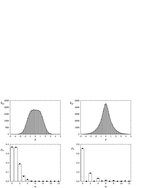
FIG. 1.: Monte Carlo simulations for a coherent state (left) and a squeezed vacuum state (right). The top graphs depict phase–averaged homodyne statistics obtained from $N=10^{5}$ runs, superposed on analytical distributions shown with solid lines. The interval $-5\leq x\leq 5$ is divided into 100 bins. The bottom graphs compare the reconstructed photon number distribution (circles) with analytical values (bars). The cut–off parameter is $K=19$.

REFERENCES

- [1] M. Munroe, D. Boggavarapu, M. E. Anderson, and M. G. Raymer, Phys. Rev. A 52, R924 (1995).
- [2] S. Schiller, G. Breitenbach, S. F. Pereira, T. Müller, and J. Mlynek, Phys. Rev. Lett. 77, 2933 (1996).
- [3] K. Banaszek and K. Wódkiewicz, Phys. Rev. A 55, 3117 (1997).
- [4] G. M. D’Ariano, C. Macchiavello, and M. G. A. Paris, Phys. Rev. A 50, 4298 (1994).
- [5] U. Leonhardt, M. Munroe, T. Kiss, Th. Richter, and M. G. Raymer, Opt. Comm. 127, 144 (1996).
- [6] G. Breitenbach, S. Schiller, and J. Mlynek, Nature 387, 471 (1997); G. Breitenbach and S. Schiller, J. Mod. Opt. 44, 2207 (1997); see also Ref. [10].
- [7] Z. Hradil, Phys. Rev. A 55, R1561 (1997).
- [8] W. T. Eadie, D. Drijard, F. E. James, M. Roos, and B. Sadoulet, Statistical Methods in Experimental Physics (North–Holland, Amsterdam, 1971), Chap. 7.
- [9] T. Opatrný, D.-G. Welsch, and W. Vogel, Phys. Rev. A 56, 1788 (1997).
- [10] S. M. Tan, J. Mod. Opt. 44, 2233 (1997).
- [11] W. H. Press, S. A. Teukolsky, W. T. Vetterling, and B. P. Flannery, Numerical Recipes in Fortran: The Art of Scientific Computing, 2nd ed. (Cambridge University Press, Cambridge, 1992), Chap. 10.