Aftershocks in Coherent-Noise Models

Abstract

The decay pattern of aftershocks in the so-called ’coherent-noise’ models [M. E. J. Newman and K. Sneppen, Phys. Rev. E54, 6226 (1996)] is studied in detail. Analytical and numerical results show that the probability to find a large event at time $t$ after an initial major event decreases as $t^{-\tau}$ for small $t$, with the exponent $\tau$ ranging from 0 to values well above 1. This is in contrast to Sneppen und Newman, who stated that the exponent is about 1, independent of the microscopic details of the simulation. Numerical simulations of an extended model [C. Wilke, T. Martinetz, Phys. Rev. E56, 7128 (1997)] show that the power-law is only a generic feature of the original dynamics and does not necessarily appear in a more general context. Finally, the implications of the results to the modeling of earthquakes are discussed.

, ,

1 Introduction

Dynamical systems which display scale-free behaviour have attracted much interest in recent years. Equilibrium thermodynamic systems do only exhibit scale-free behaviour for a subset of the parameter space of measure zero (the critical values of the parameters). Nevertheless, in nature scale-free systems can be found in abundant variety (earthquakes [1], avalanches in rice-piles [2], infected people in epidemics [3], jams in Internet traffic [4], extinction events in Biology [5], life-times of species [6] and many more. See also [7] and the references therein). The origin of this abundance lies probably in the broad variety of systems far from equilibrium that can be found in nature. With the onset of non-equilibrium dynamics, new mechanisms come into play which seem to make scale-free behaviour a generic feature of many systems. However, unlike equilibrium thermodynamics, where scaling is thoroughly understood [8, 9], for non-equilibrium dynamical systems there does not yet exist a unified theory of scale-free phenomena (apart from non-equilibrium phase transitions). There do, however, exist several distinct classes of systems with generic scale-free dynamic.

One of the first ideas to explain scale-free behaviour in a large class of dynamical systems was the notion of Self-Organized Criticality (SOC) proposed by Bak, Tang and Wiesenfeld in 1987 [10, 11]. They proposed that certain systems with local interactions can, under the influence of a small, local driving force, self-organize into a state with diverging correlation length and therefore scale-free behaviour. This state is similar to the ordinary critical state that arises at the critical point in phase transitions, although no fine-tuning of parameters is necessary to reach it. Since 1987 literally thousands of research papers have been written concerning SOC (for a review see [12]), and many different dynamical systems have been called SOC (e.g. [13, 14, 15, 16, 17]), mostly just because they showed some power-law distributed activity patterns. Recently [18] it has become clear that several SOC models (sandpile models, forest-fire models) can be understood in terms of ordinary nonequilibrium critical phenomena (like e.g. [19]). Driving rate and dissipation act as critical parameters. The critical value, however, is 0. Therefore, it suffices to choose a small driving rate and dissipation to fine-tune the system to the critical point, and this choice is usually implicit in the definition of the model.

Scale-free behaviour does not, however, depend crucially on some sort of critical phenomenon. A simple multiplicative stochastic process (MSP) of the form

$$x(t+1)=a(t)x(t)+b(t)\,,$$ (1)

where $a(t)$ and $b(t)$ are random variables, can produce a random variable $x(t)$ with a probability-density function (pdf) with power-law tail [21, 22, 23, 24, 25]. In processes of this type, the power-law appears under relatively weak conditions on the pdf’s of $a(t)$ and $b(t)$, thus making the intermittend behaviour a generic feature of such models. Applications of Eq. (1) can be found in population dynamics with external sources [25], epidemics [3], price volatility in economics [26], and others.

Another class of models with a very simple and robust mechanism to produce scale-free behaviour has been introduced recently by Newman and Sneppen [27]. These so called ’coherent-noise’ models consist of a large array of ’agents’ which are forced to reorganize under externally imposed stress. In their simplest form, coherent-noise models do not have any interactions between the agents they consist of, and hence, certainly do not display criticallity. Nevertheless, these models show a power-law distribution of the reorganization events with a wide range of different exponents [28], depending on the special implementation of the basic mechanism. Moreover they display power-law distributions in several other quantities, e.g., the life-time distribution of the agents. These models have been used to study earthquakes [27], rice piles [27], and biological extinction [29, 30, 31, 32].

Coherent-noise models have a feature that usually is not present in SOC models and is never present in MSP’s, which is the existence of aftershocks. In most coherent-noise models the probability for a big event to occur is very much increased immediately after a previous big event and then decays with a power-law. This leads to a fractal pattern of events that are followed by smaller ones which themselves are followed by even smaller ones and so on. In most SOC models and all MSP’s, on the contrary, the state of the system is statistically identical before and after a big event. Therefore in these models no aftershocks are visible.

The existence or non-existence of aftershock events should be easily testable in natural systems. This could provide a means to decide what mechanism is most likely to be the cause for scale-free behaviour in different situations [28]. But to achieve this it is important to have a deep understanding of the decay-pattern of the aftershock events.

The goal of the present paper is to investigate in detail the aftershock dynamics of coherent-noise models. We concentrate mainly on the original model introduced by Newman and Sneppen because there can be obtained several analytical results. We find a power-law decrease in time of the aftershocks’ probability to appear, as has been found already in [28]. But unlike stated there, we can show that the exponent does indeed depend on the microscopic details of the simulation. We find a wide range of exponents, from 0 to values well above 1, whereas in [28] the authors report only the value 1.

2 The model

We will now describe the model introduced by Newman and Sneppen [27]. The system consists of $N$ units or ’agents’. Every agent $i$ has a threshold $x_{i}$ again external stress. The thresholds are initially chosen at random from some probability distribution $p_{\rm thresh}(x)$. The dynamics of the system is as follows:

1. A stress $\eta$ is drawn from some distribution $p_{\rm stress}(\eta)$. All agents with $x_{i}\leq\eta$ are given new random thresholds, again from the distribution $p_{\rm thresh}(x)$.

2. A small fraction $f$ of the agents is selected at random and also given new thresholds.

3. The next time-step begins with (i).

Step (ii) is necessary to prevent the model from grinding to a halt. Without this random reorganization the thresholds of the agents would after some time be well above the mean of the stress distribution and average stress could not hit any agents anymore.

The most common choices for the threshold and stress distributions are a uniform threshold distribution and some stress distribution that is falling off quickly, like the exponential or the gaussian distribution. Under these conditions (with reasonably small $f$) it is guaranteed that the distribution of reorganization events that arises through the dynamics of the system will be a power-law.

There are several possibilities to extend the model to make it more general, without loss of the basic features. Two extensions that have been studied by Sneppen and Newman [28] are

• a lattice version where the agents are put on a lattice and with every agent hit by stress its nearest neighbours undergo reorganization, even if their threshold is above the current stress level.

• a ’multi-trait’ version where, instead of a single stress, there are $M$ different types of stress, i.e. the stress becomes a $M$-dimensional vector $\boldsymbol{\eta}$. Accordingly, every agent has a vector of thresholds $\mathbf{x_{i}}$. An agent has to move in this model whenever at least one of the components of the threshold vector is exceeded by the corresponding component of the stress vector.

An extension that is especially important for the application of coherent noise models to biological evolution and the dynamics of mass extinctions has been studied recently by Wilke and Martinetz [32]. In biology it is not a good assumption to keep the number of agents (in this case species) constant in time. Rather, species which go extinct should be removed, and there should be a steady regrowth of new species. In a generalized model, the system size is allowed to vary. Agents that are hit by stress are removed from the system completely, but at the end of every time-step a number $\Delta N$ of new agents is introduced into the system. Here $\Delta N$ is a function of the actual system size $N$, the maximal system size $N_{\max}$ and some growth rate $g$. Wilke and Martinetz have studied in detail the function

$$\Delta N=\frac{NN_{\max}e^{g}}{N_{\max}+N(e^{g}-1)}-N\,,$$ (2)

which resembles logistic growth. In the limit $g\rightarrow\infty$ their model reduces to the original one by Newman and Sneppen. In the following we will refer to the original model as the ’infinite-growth version’ and to the model introduced by Wilke and Martinetz as the ’finite-growth version’.

3 Analysis of the aftershock structure

We base our analysis of the aftershock structure on the meassurement-procedure proposed by Sneppen and Newman [28]. They drew a histogram of all the times whenever an event of size $\geq$ some constant $s_{1}$ happened after an initial event of size $\geq$ some constant $s_{0}$, for all events $\geq s_{0}$. Consequently, we measure the frequency of events larger than $s_{1}$ occuring exactly $t$ time-steps after an initial event larger than $s_{0}$, for all times $t$. This means that we consider sequences of events in the aftermath of initial large events. Normalized appropriately, our measurement gives just the probability to find an event $\geq s_{1}$ at time $t$ after some arbitrarily chosen event $\geq s_{0}$. For this to make sense in the context of aftershocks we usually have $s_{0}>s_{1}$. Throughout the rest of this paper we use $s_{0}$ and $s_{1}$ as percentage of the maximal system size. Therefore a value $s_{0}=1$ for example means that we are looking for initial events which span the whole system.

We will denote the probability to find an event of size $s\geq s_{1}$ at time $t$ after a previous large event by $P_{t}(s\geq s_{1})$. In order to keep the notation simple we omit the constant $s_{0}$. It will be clear from the context what $s_{0}$ we use in different situations. Note that $P_{t}(s\geq s_{1})$ is not a probability distribution, but a function of time $t$. Therefore, every increase or decrease of $P_{t}(s\geq s_{1})$ in time will indicate correlations between the initial event and the subsequent aftershocks. For $t\rightarrow\infty$ we expect all correlations to disappear, and hence $P_{t}(s\geq s_{1})$ to tend towards a constant.

It is possible to obtain some analytical results about the probability $P_{t}(s\geq s_{1})$ if we restrict ourself to the model with infinite growth and a special choice for the threshold and stress distributions. If not indicated otherwise, throughout the rest of this section we assume $p_{\rm thresh}(x)$ to be uniform between 0 and 1, and the stress distribution to be exponential: $p_{\rm stress}(\eta)=\exp(-\eta/\sigma)/\sigma$.

Furthermore, we focus on the case $s_{0}=1$. That means that we are looking at the events in the aftermath of an initial event of ’infinite’ size, an event that spans the whole system. This is a reasonable situation because we use a uniform threshold distribution. In this case there is a finite probability to generate a stress $\eta$ which exceedes the largest threshold, thus causing the whole system to reorganize. For some of the examples presented in Section 4 the probability to find an infinite event is even higher than $10^{-5}$. This probability can be considered relatively large in a system where one has to do about $10^{6}-10^{9}$ time-steps to get a good statistics.

3.1 Mean-field solution

The exact way to calculate $P_{t}(s\geq s_{1})$ is the following. One has to compute the distribution $\rho_{t-1}^{\eta_{1},\eta_{2},\dots,\eta_{t-1}}(x)$ which is the distribution that arises if after the big event at time $t=0$ a sequence of stress values $\eta_{1},\eta_{2},\dots,\eta_{t-1}$ is generated during the following time steps. Then the equation

$$\int\limits_{0}^{x_{t}(\eta_{1},\eta_{2},\dots,\eta_{t-1},s_{1})}\rho_{t-1}^{\eta_{1},\eta_{2},\dots,\eta_{t-1}}(x^{\prime})\,dx^{\prime}=s_{1}$$ (3)

has to be solved. That gives the quantity $x_{t}(\eta_{1},\eta_{2},\dots,\eta_{t-1},s_{1})$, the threshold that has to be exceeded by the stress at time $t$ to generate an event $\geq s_{1}$. From the stress distribution one can then calculate the corresponding probability $P_{t}^{\eta_{1},\eta_{2},\dots,\eta_{t-1}}(s\geq s_{1})$. Finally the average over all possible sequences $\eta_{1},\eta_{2},\dots,\eta_{t-1}$ has to be taken to end up with the exact solution for $P_{t}(s\geq s_{1})$. Obviously there is no hope doing this analytically.

Instead of the exact solution for $P_{t}(s\geq s_{1})$ we can calculate a mean-field solution if we average over all possible sequences $\eta_{1},\eta_{2},\dots,\eta_{t-1}$ before we solve Eq. (3). Note that in this context, the notion mean-field does not stand for the average state of the system, which does not tell us anything about aftershocks, but for the average fluctuations typically found in a time-intervall $\Delta t$. These average fluctuations are a measure for the return to the average state, after a large event has caused a significant departure from it. Consequently, the mean-field solution is time-dependent. For $\Delta t\rightarrow\infty$, the time-dependent mean-field threshold distribution converges to the average threshold distribution, denoted by $\bar{\rho}(x)$ in [28]

In Appendix A, we show that the averaging over all fluctuations in a time intervall of $t$ time-steps equals to $t$ times iterating the master-equation. Therefore, to calculate the mean-field solution for $P_{t}(s\geq s_{1})$ we have to insert $\rho_{t}(x)$, the $t$-th iterate of the master-equation, into Eq. (3). The details of this calculation are given in Appendix B.

3.2 Approximation for $\tau$

In this paragraph we will calculate the dependency of the exponent $\tau$ on $s_{1}$ under the assumption that the probability to find aftershocks decays indeed as a power-law, i.e. that we can assume $P_{t}(s\geq s_{1})\sim t^{-\tau}$. A fairly simple argument shows that for the probability $P_{t}(s\geq s_{1})$ to decrease as a power-law the exponent $\tau$ must be proportional to $1-s_{1}$ for $s_{1}$ not too small. Again we concentrate on exponentially distributed stress only.

We begin with an approximation of the quantity $x_{t}(s_{1})$, which is the average threshold at time $t$ above which a stress value must lie to trigger an event of size $\geq s_{1}$. In the mean-field approximation, $x_{t}(s_{1})$ is defined by the equation

$$\int\limits_{0}^{x_{t}(s_{1})}\rho_{t}(x)\,dx=s_{1}\,.$$ (4)

Because $\rho_{t}(x)$ and $s_{1}$ are normalized, we can rewrite this equation (again we assume $p_{\rm thresh}(x)$ to be uniform between 0 and 1):

$$\int\limits_{x_{t}(s_{1})}^{1}\rho_{t}(x)\,dx=1-s_{1}\,.$$ (5)

For the most reasonable stress distributions the distribution of the agents $\rho_{t}(x)$ forms a plateau in the region close to $x=1$. Therefore for sufficient large $s_{1}$ we can approximate the integral in Eq. (5) by substituting $\rho_{t}(x)$ with its value at $x=1$, which is $\rho_{t}(1)$. Eq. (5) then becomes

$$\Big{(}1-x_{t}(s_{1})\Big{)}\rho_{t}(1)=1-s_{1}\,.$$ (6)

The values $\rho_{t}(1)$ are a function of $t$. We define

$$R(t):=\rho_{t}(1)$$ (7)

and find for $x_{t}(s_{1})$:

$$x_{t}(s_{1})=\frac{s_{1}-1+R(t)}{R(t)}\,.$$ (8)

The probability $P_{t}(s\geq s_{1})$ now becomes

$$P_{t}(s\geq s_{1})=\exp\Big{(}-\frac{x_{t}(s_{1})}{\sigma}\Big{)}=\exp\Big{(}-\frac{s_{1}-1+R(t)}{\sigma R(t)}\Big{)}\,.$$ (9)

The principal idea to derive a relation between $\tau$ and $s_{1}$ is as follows. The function $R(t)$ is obviously independent of $\tau$ and $s_{1}$. We make the ansatz $P_{t}(s\geq s_{1})\sim t^{-\tau}$, rearrange Eq. (9) for $R(t)$ and then get a condition on $\tau$ and $s_{1}$ since they should cancel exactly. Hence we have to solve the equation

$$at^{-\tau}=\exp\Big{(}-\frac{s_{1}-1+R(t)}{\sigma R(t)}\Big{)}\,,$$ (10)

where $a$ is the constant of proportionality. We take the logarithm on both sides to get

$$\ln a-\tau\ln t=-\frac{s_{1}-1+R(t)}{\sigma R(t)}$$ (11)

and finally

$$R(t)=\frac{1-s_{1}}{1+\sigma\ln a-\tau\sigma\ln t}\,.$$ (12)

This is of the form $c_{1}/(c_{2}-\ln t)$, where

$$c_{1}=\frac{1-s_{1}}{\tau\sigma}$$ (13)

and

$$c_{2}=\frac{1+\sigma\ln a}{\tau\sigma}\,.$$ (14)

For every function of the form $c_{1}/(c_{2}-\ln t)$, the constants $c_{1}$ and $c_{2}$ are unique, as can be seen if we write

$$\frac{c_{1}}{c_{2}-\ln t}=\frac{c_{1}}{\ln\frac{\exp c_{2}}{t}}\,.$$ (15)

A change in $c_{2}$ results in a rescaling of the variable $t$, while a change in $c_{1}$ results in a rescaling of the whole function. Consequently, neither $c_{1}$ nor $c_{2}$ can depend on $\tau$ or $s_{1}$. This can be seen as follows. If, e.g., $c_{1}$ depended on $s_{1}$, then a change in $s_{1}$ would rescale the function $R(t)$. But this function is independent of $s_{1}$ according to its definition (Eq. (7)). Hence $c_{1}$ must be independent of $s_{1}$ in itself. A similar argument holds for the variable $c_{2}$. Therefore, $s_{1}$ and $\tau$ must cancel exactly in Eq. (13). This leads to the condition

$$\tau=\frac{1-s_{1}}{\sigma c_{1}}\sim(1-s_{1})\,.$$ (16)

Up to now we have not done any assumptions about the size of the first big event after which we are measuring the subsequent aftershocks. Therefore the proportionality $\tau\sim(1-s_{1})$ should hold in general, as long as $s_{1}$ is not too small. If we additionally assume the inital event to have infinite size ($s_{0}=1$) we can easily calculate the constant $a$ in Eq. (10). The meaning of this constant is the probability to get an event of size $\geq s_{1}$ immediately after the initial big event, as can be seen by setting $t=1$:

$$P_{1}(s\geq s_{1})=a1^{-\tau}=a\,.$$ (17)

For the case $s_{0}=1$ the distribution of thresholds $\rho_{0}(x)$ is uniform and thus

$$a=\exp(-\frac{x_{1}(s_{1})}{\sigma})=\exp(-\frac{s_{1}}{\sigma})\,.$$ (18)

With Eqs. (9), (10), (13), and (18) we can write the probability $P_{t}(s\geq s_{1})$ as

$$P_{t}(s\geq s_{1})=e^{-s_{1}/\sigma}t^{-(1-s_{1})/(\sigma c_{1})}\,.$$ (19)

In Section 4 we will find numerically that $c_{1}=\sigma^{-1}$, and therefore $\tau=1-s_{1}$.

3.3 Limiting cases

For two limiting cases we can deduce the behaviour of the exponent $\tau$ regardless of the stress distribution. We begin with the case $s_{0}=1$, $s_{1}\rightarrow 1$. From Eq. (16) we find that $\tau\rightarrow 0$ as $s_{1}\rightarrow 1$ under the assumption of an exponential stress distribution. But this result is more general. For $s_{1}=1$ the probability $P_{t}(s\geq s_{1})$ reads simply

$$P_{t}(s\geq 1)=\int\limits_{1}^{\infty}\!dx\,p_{\rm stress}(x)$$ (20)

and hence is constant in time. Consequently we have $\tau=0$ for any stress distribution. From continuity we have $\tau\rightarrow 0$ as $s_{1}\rightarrow 1$.

A similar argument holds when either $s_{0}$ or $s_{1}$ approaches 0. For $s_{0}=0$, the probability $P_{t}(s\geq s_{1})$ reduces to the mean probability to find an event of size $s\geq s_{1}$. Hence $\tau=0$. For $s_{1}=0$, the probability $P_{t}(s\geq s_{1})$ becomes 1, because an event of size at least zero can be found in every time step. Hence also in this case $\tau=0$. From continuity we have again $\tau\rightarrow 0$ as either $s_{0}\rightarrow 0$ or $s_{1}\rightarrow 0$.

4 Numerical results

In the previous section we have focused on the behaviour of the system in the aftermath of an infinite event. This situation is not only analytically tractable, but it also makes it simpler to obtain good numerical results. If we want to measure the probability to find aftershocks following events exceeding some finite but large $s_{0}$, we have to wait a long time for every single measurement since the number of those large events vanishes with a power-law. This makes it hard to get a good statistics within a reasonable amount of computing time. If, on the other hand, we focus on the situation of an infinite initial event, we can simply initialize the agents with the uniform threshold distribution, take the measurement up to the time $t$ we are interested in and repeat this procedure until the desired accuracy is reached. Unless stated otherwise, the results reported below have been obtained in this way, and with exponentially distributed stress.

The $t$-th iteration of the master-equation should give exactly the average distribution of the agent’s thresholds at time $t$. In Fig. 1 it can be seen that this is indeed the case. The points, which represent simulation results, lie exactly on the solid lines, which stem from the exact analytical calculation.

The mean-field approximation for $P_{t}(s\geq s_{1})$ should be valid if the agent’s distribution at time $t$ does not fluctuate too much about the average distribution $\rho_{t}(x)$. Since there are many more small events than big ones the fluctuations should occur primarily in the region of small $x$. Consequently we expect the mean-field approximation to be valid for large $s_{1}$, and to break down for small $s_{1}$. Fig. 2 shows that already for moderately large $s_{1}$ the mean-field approximation captures the behaviour of $P_{t}(s\geq s_{1})$, with a slight tendency to underestimate the results of the measurement. Note that the statistics is becoming worse with increasing $s_{1}$ due to the rapidly decreasing probability to find any events of size $\geq s_{1}$ for large $s_{1}$.

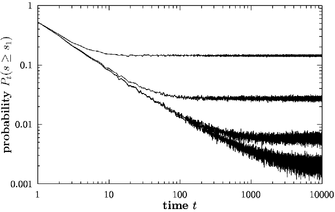
Figure 3: The probability $P_{t}(s\geq s_{1})$ in simulations with $\sigma=0.1$, $s_{1}=0.06$ and several different values for $f$ (from bottom to top: $f=10^{-4}$, $f=10^{-3}$, $f=10^{-2}$, $f=10^{-1}$).

In Fig. 3 a measurement of the probability $P_{t}(s\geq s_{1})$ is presented for a number of simulations with different values of the parameter $f$. As it can be seen, the parameter $f$ does not affect the exponent of the power-law, but limits the region where scaling can be observed. Note the difference between the effect seen here and typical cut off effects in the theory of phase transitions. The quantity $P_{t}(s\geq s_{1})$ is not a probability distribution, but a time dependent probability, which tends towards a constant for $t\rightarrow\infty$. Therefore, we do not see an exponential decrease at the cut off timescale. Instead, the probability $P_{t}(s\geq s_{1})$ levels out to the time-averaged value $P(s\geq s_{1})$, which is the average probability to find events of size $s\geq s_{1}$.

In section 3.2 we showed that $\tau\sim 1-s_{1}$, under the condition of a sufficiently large $s_{1}$. Simulations indicate that the constant of proportionality is just 1, which means the constant $c_{1}$ in Eq. (13) equals $\sigma^{-1}$. If this hypothesis is true, Eq. (19) becomes

$$P_{t}(s\geq s_{1})=e^{-s_{1}/\sigma}t^{-(1-s_{1})}\,.$$ (21)

This means, a rescaling of the form

$$P_{\rm scaled}=\left(\frac{P_{t}(s\geq s_{1})}{e^{-s_{1}/\sigma}}\right)^{1/(s_{1}-1)}$$ (22)

should yield a functional dependency $P_{\rm scaled}(t)=t^{-1}$. Fig. 4 shows the results of such a rescaling for different $\sigma$ and $s_{1}$. All the data-points lie exactly on top of each other in the region where the statistics is good enough (about $t<100$). We find that for $\sigma$ up to 0.1, Eq. (21) is very accurate for $s_{1}$ between about 0.1 and 1. With smaller $\sigma$, Eq. (21) holds even for much smaller $s_{1}$.

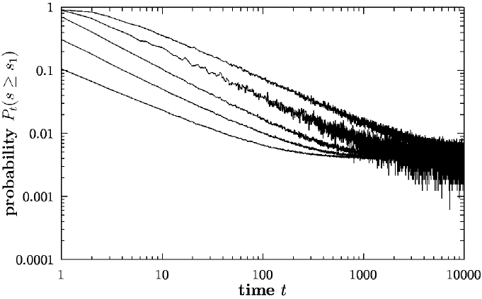
Figure 6: The probability $P_{t}(s\geq s_{1})$ after an initial finite event. Parameters are $\sigma=0.05$, $f=10^{-5}$, $s_{1}=3\times 10^{-4}$, and, from bottom to top, $s_{0}=5\times 10^{-4}$, $s_{0}=2\times 10^{-3}$, $s_{0}=0.01$, $s_{0}=0.1$ and $s_{0}=1$.

The situation becomes more complicated if we study the sequence of aftershocks caused by an initial event of finite size. The probability to find an event of size $s\geq s_{1}$ after some initial event of size $s\geq s_{0}$ decreases with a power-law, but the exponent is not a simple function of $s_{1}$. Rather, it depends on $s_{0}$ as well. In Fig. 6 we have displayed the results of a measurement with $s_{1}=3\times 10^{-4}$ and several different $s_{0}$, ranging from $5\times 10^{-4}$ to 1. The curve for $s_{0}=1$ has been obtained with the method described at the beginning of this section. We find that the aftershocks’ decay pattern for $s_{0}<1$ continuously approaches the one for $s_{0}=1$ as $s_{0}\rightarrow 1$. This shows that it is indeed justified to study the system in the aftermath of an infinite initial event and then to extrapolate to finite but large initial events. Note that in Fig. 6, $s_{1}$ is so small that Eq. (21) does not hold anymore.

Sneppen and Newman have argued that the decay pattern of the aftershocks is independent of the respective stress distribution. Our results do not support that. Despite the fact that the exponent of the power-law seems to be independent of $\sigma$ in the case of exponential stress, as we could show above, the exponent is not independent of the functional dependency of the stress distribution. If we impose, for example, gaussian stress with mean 0 and variance $\sigma$, we find (Fig. 5) exponents larger than 1 for moderate $s_{1}$. We do event find a qualitatively new behaviour of the system. The exponent is getting larger with increasing $s_{1}$, as opposed to the exponent getting smaller for exponential stress. Of course, this can only be true for intermediate $s_{1}$. Ultimately, we must have $\tau\rightarrow 0$ for $s_{1}\rightarrow 1$.

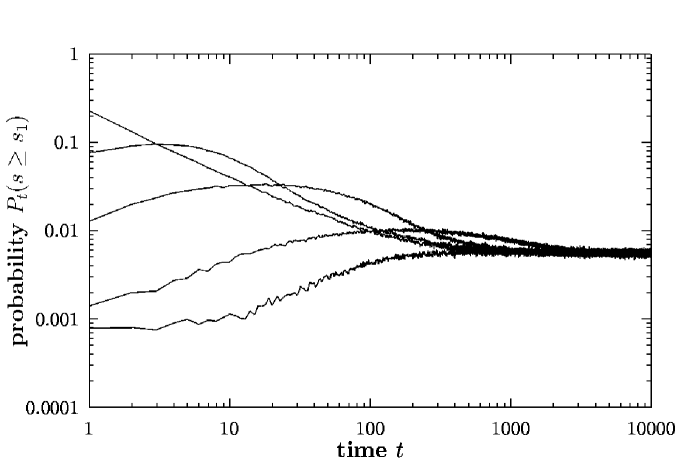
Figure 7: The probability $P_{t}(s_{1}\geq 3\times 10^{-4})$ after an event of size $s_{0}\geq 0.001$ in a simulation with finite logistic growth. Parameters are $\sigma=0.5$, $f=10^{-5}$, and, from bottom to top, $g=2\times 10^{-4}$, $g=2\times 10^{-3}$, $g=2\times 10^{-2}$ $g=2\times 10^{-1}$, $g=10$. A power-law can only be seen for relatively large growth rates. For small growth-rates, the probability to find aftershocks is reduced significantly.

Finally, we present some results about systems with finite growth. In these systems, there exists some competitive dynamics between the removal of agents with small thresholds through stress and their regrowth. Aftershocks appear in the infinite growth model because the reorganization event leaves a larger proportion of agents in the region of small thresholds, thus increasing the probability for succeding large events. In the finite growth version, on the contrary, this can happen only if the regrowth is faster than the constant removal of agents with small thresholds through average stress. If the regrowth is too slow, the probability to find large events actually is decreased in the aftermath of an initial large event. The interplay between these two mechanisms is shown in Fig. 7. The regrowth of species is done according to Eq. (2). For a small growth-rate $g$, the probability to find aftershocks is reduced significantly, and it aproaches the equilibrium value after about 100 time-steps. With larger $g$, the probability $P_{t}(s\geq s_{1})$ increases in time until a maximum well above the equilibrium level is reached, and then decreases again. The maximum moves to the left to earlier times $t$ with increasing $g$. When $g$ is so large that the maximum coincides with the post initial event, the original power-law is restored. Note that, as in the case of infinite growth, the measurement depends on the choice of the parameters $s_{0}$ and $s_{1}$. Consequently, with a different set of parameters the curves will look different, and the maximum will appear at a different time. Nevertheless, we find that the qualitative behaviour is not altered if we change $s_{0}$ or $s_{1}$.

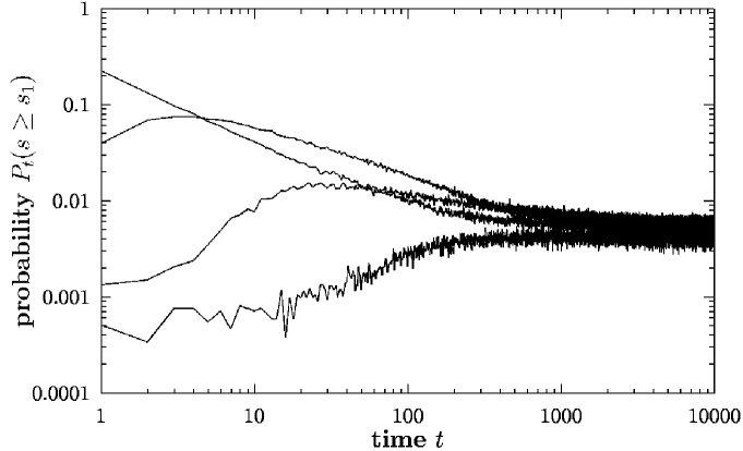
Figure 8: The probability $P_{t}(s_{1}\geq 3\times 10^{-4})$ after an event of size $s_{0}\geq 0.001$ in a simulation with finite linear growth. Parameters are $\sigma=0.5$, $f=10^{-5}$, and, from bottom to top, $g=10^{-5}$, $g=\times 10^{-4}$, $g=\times 10^{-3}$, $g=10$. Aftershocks are seen for much smaller growth rates than in the version with logistic growth.

Instead of logistic growth, we can also think of linear growth, i.e. $\Delta N=gN_{\max}$, where $g$ is again the growth rate. In order to keep the system finite, we stop the regrowth whenever the system size $N$ exceedes the maximal system size $N_{\max}$. In such a system, aftershocks can be seen for much smaller growth rates (Fig. 8). Note that apart from the growth rate, all other settings are identical in Fig. 7 and Fig. 8. Linear growth refills the system much quicker than logistic growth with the same growth rate. Therefore the time intervall in which aftershocks are suppressed is much shorter for linear growth.

5 Conclusion

We could show in the present paper that the decay pattern of the aftershock events depends on the details of the measurement. Although the qualitative features remain the same for different parameters $s_{0}$ and $s_{1}$ (e.g. a power-law decrease in the infinite-growth version), the quantitative features vary to a large extend. The exponent $\tau$ of the power-law is significantly affected by an alteration of $s_{0}$ or $s_{1}$. Therefore the measurement-procedure proposed by Sneppen and Newman can reveal the complex structure of aftershock-events only if the change of the measured decay pattern with varying $s_{0}$ and $s_{1}$ is recorded over a reasonably large intervall of different values. This should be considered in a possible comparison between the aftershocks’ decay pattern from a model and from experimental data. A more in-depth analysis could probably be achieved with the formalism of multifractality (see e.g. [33]).

We found the aftershocks’ decay pattern to vary with different stress distributions. This is in clear contrast to Sneppen and Newman. They reported a power-law with exponent $t\approx 1$ for the infinite growth version, independent of the respective stress distribution they used. The question remains why Sneppen and Newman measured such an exponent in all their simulations. The answer to this lies in the fact that they did only simulations with $s_{0}<1$. For the reasons explained at the beginning of Section 4, under this condition one has to choose a relatively small $s_{0}$, and accordingly, a very small $s_{1}$. This causes the measurement almost inevitably to lie in the intermediate region between the limiting cases of Sec. 3.3. In this region, for the most reasonable stress distributions and a large array of different values for $s_{0}$ and $s_{1}$, we find indeed exponents around 1.

The application of coherent-noise models to earthquakes has been discussed in [27]. Two very important observations regarding earthquakes, the Gutenberg-Richter law [34, 35] and Omori’s law [36], can be explained easily with a coherent-noise model. The Gutenberg-Richter law states that earthquake magnitudes are distributed according to a power-law. Omori’s law, which interests us here, is a similar statement for the aftershocks’ decay pattern of earthquakes. In the data from real earthquakes, the number of events larger than a certain magnitude $M_{1}$ decreases as $t^{-\tau}$ in the aftermath of a large initial earthquake. Consequently, we can only apply infinite-growth coherent-noise models to earthquakes. But this is certainly no drawback, since we expect the thresholds against movement at various points along a fault (with which we identify the agents of the coherent-noise model) to reorganize almost instantaneously during an earthquake.

The exponent $\tau$ is not universal, but can vary significantly, e.g., in [1] from $\tau=0.80$ to $\tau=1.58$. This would cause problems if the statement was true that for coherent-noise models we have $\tau\approx 1$. But as we could show above, the exponent can assume values in the observed range, depending on the stress distribution, the size of the initial event, and the lower cut-off (which we called $M_{1}$ for earthquakes and $s_{1}$ throughout the rest of the paper).

For a further comparison, it should be interesting to study the dependency of the exponent $\tau$ on variation of the cut-off $M_{1}$ in real data. We are only aware of a single work where that has been done [37]. Interestingly, the authors do not find a clear dependency $\tau(M_{1})$. Nevertheless, this is not a strong evidence against coherent-noise models, since the aftershock series analysed in [37] consists mainly of very large earthquakes with magnitude between 6 and about 8, which does not allow a sufficient variation of $M_{1}$. Statistical variations in the exponent $\tau$ are probably larger for this aftershock series than the possible variations because of an assumed $\tau(M_{1})$ dependency.

Numerical simulations of the finite-growth version have revealed a much more complex structure of aftershock events than present in the infinite-growth version. The competition between regrowth of agents and agent removal through reorganization events leads to a pattern where the probability to find events after an initial large event is suppressed for short times, enhanced for intermediate times and then falls off to the background level for long times. This observation can be important for the application of coherent-noise models to biological extinction. It might be possible to identify a time of reduced and a time of enhanced extinction activity in the aftermath of a mass extinction event in the fossil record. This would be a good indication for biological extinction to be dominated by external influences (coherent-noise point of view) rather than by coevolution (SOC point of view).

Appendix A Rederivation of the master-equation

In this appendix we are interested in the average state a coherent-noise system will be found in several time-steps after some initial state with threshold distribution $\rho_{t_{0}}(x)$. Our calculations will lead to a rederivation of the master-equation for coherent-noise systems. Although a master-equation has already been given for the infinite-growth version and has been generalized to the finite-growth version, these master-equations have not been derived in a stringent way, but just have been written down intuitively. Our calculation will confirm the main terms of the previously used equations, but we will find an additional correcting term that becomes important for large $f$.

Consider the case of infinite growth. At time $t_{0}$ the threshold-distribution may be $\rho_{t_{0}}(x)$. We construct the distribution $\rho_{t_{0}+1}^{\eta}(x)$, which is the distribution that arises at time $t_{0}+1$ if a stress $\eta$ is generated at time $t_{0}$. A stress $\eta$ will cause a proportion $s_{\eta}=\int_{0}^{\eta}\!dx\,\rho_{t_{0}}(x)$ of the agents to move. We have to distinguish two regions. For $x<\eta$, all agents are removed. Then they are redistributed according to $s_{\eta}p_{\rm thresh}(x)$. A small fraction $f$ of the agents is then mutated, which results in

$$\rho_{t_{0}+1}^{\eta}(x)=(1-f)s_{\eta}p_{\rm thresh}(x)+fp_{\rm thresh}(x)\quad;\;x<\eta\,.$$ (23)

For $x\geq\eta$, the redistribution of the agents gives $\rho_{t_{0}}(x)+s_{\eta}p_{\rm thresh}(x)$. With the subsequent mutation we obtain:

$$\rho_{t_{0}+1}^{\eta}(x)=(1-f)\Big{(}\rho_{t_{0}}(x)+s_{\eta}p_{\rm thresh}(x)\Big{)}+fp_{\rm thresh}(x)\quad;\;x\geq\eta\,.$$ (24)

We take the average over $\eta$ to get the distribution $\rho_{t_{0}+1}(x)$ that will on average be found one time-step after $\rho_{t_{0}}(x)$:

$$\rho_{t_{0}+1}(x) =\int\limits_{0}^{\infty}\!d\eta\,p_{\rm stress}(\eta)\rho_{t_{0}+1}^{\eta}(x)$$

$$=\int\limits_{0}^{\infty}\!d\eta\,p_{\rm stress}(\eta)p_{\rm thresh}(x)\Big{[}(1-f)\int\limits_{0}^{\eta}\rho_{t_{0}}(x^{\prime})dx^{\prime}+f\Big{]}$$

$$\qquad+\int\limits_{0}^{x}\!d\eta\,p_{\rm stress}(\eta)\rho_{t_{0}}(x)(1-f)$$

$$=p_{\rm thresh}(x)\Big{[}f+(1-f)\int\limits_{0}^{\infty}\!d\eta\,p_{\rm stress}(\eta)\int\limits_{0}^{\eta}\rho_{t_{0}}(x^{\prime})dx^{\prime}\Big{]}$$

$$\qquad+\rho_{t_{0}}(x)(1-f)(1-p_{\rm move}(x))\,.$$ (25)

Here, $p_{\rm move}(x)$ is the probability for an agent with threshold $x$ to get hit by stress, viz. $p_{\rm move}(x)=\int_{x}^{\infty}\!dx^{\prime}\,p_{\rm stress}(x^{\prime})$. To proceed further we have to interchange the order of integration in the remaining double integral. Note that $\int_{0}^{\infty}\!d\eta\,\int_{0}^{\eta}\!dx^{\prime}=\int_{0}^{\infty}\!dx^{\prime}\,\int_{x^{\prime}}^{\infty}\!d\eta$, and therefore

$$\rho_{t_{0}+1}(x) =p_{\rm thresh}(x)\Big{[}f+(1-f)\int\limits_{0}^{\infty}\!dx^{\prime}\,\int\limits_{x^{\prime}}^{\infty}\!d\eta\,p_{\rm stress}(\eta)\rho_{t_{0}}(x^{\prime})\Big{]}$$

$$\qquad+\rho_{t_{0}}(x)(1-f)(1-p_{\rm move}(x))$$

$$=p_{\rm thresh}(x)\Big{[}f+(1-f)\int\limits_{0}^{\infty}\!dx^{\prime}\,\rho_{t_{0}}(x^{\prime})p_{\rm move}(x^{\prime})\Big{]}$$

$$\qquad+\rho_{t_{0}}(x)(1-f)(1-p_{\rm move}(x))$$

$$=p_{\rm thresh}(x)\int\limits_{0}^{\infty}\!dx^{\prime}\,\Big{(}f+(1-f)p_{\rm move}(x^{\prime})\Big{)}\rho_{t_{0}}(x^{\prime})$$

$$\qquad+\rho_{t_{0}}(x)(1-f)(1-p_{\rm move}(x))$$ (26)

We are thus led to the master-equation

$$\Delta\rho_{t}(x)=\Big{(}-f-p_{\rm move}(x)+fp_{\rm move}(x)\Big{)}\rho_{t}(x)+Ap_{\rm thresh}(x)\,,$$ (27)

where $A$ is the normalization constant $\int_{0}^{\infty}\!dx^{\prime}\,(f+(1-f)p_{\rm move}(x^{\prime}))\rho_{t}(x^{\prime})$.

We notice the appearance of the term $fp_{\rm move}(x)$ which was not present in the master-equation used by Sneppen and Newman. The term arises if one takes into account the fact that the agents which are hit by stress get new thresholds before the mutation takes place. Therefore every agent with threshold $x$ has the probability $fp_{\rm move}(x)$ to get two new thresholds in one time-step. But obviously this is exactly the same as geting only one new threshold. Consequently, the term $fp_{\rm move}(x)$ has to be present to avoid double-counting of those agents which are hit both by stress and by mutation. Nevertheless, this term does not affect the scaling behaviour of the system, because the derivation of the event size distribution in [28] has been done under the assumption $f\ll 1$.

Eq. (A) gives the average state of the system one time-step after the initial state $\rho_{t_{0}}(x)$. If we are interested in the average state $t$ time-steps after the initial state, we have to repeat the calculations in Eqs. (23)-(A) $t$ times. Since all averages in these calculations can be taken independently, this is exactly the same as $t$ times iterating the master-equation (27).

Appendix B Calculation of the mean-field solution.

We assume that at time $t=0$ a big event takes place and produces the distribution $\rho_{0}(x)$. If we apply the master-equation (27) $t$ times to this distribution $\rho_{0}(x)$, we will end up with a distribution $\rho_{t}(x)$ that tells us the average state of the system at time $t$ after the big event.

In the following we will use

$$T(x):=(1-f)(1-p_{\rm move}(x))$$ (28)

and write $A_{t}$ for the normalization constant that appears on the right-hand side of Eq. (27) at time $t$. The average distribution at time $t$ then becomes

$$\rho_{t}(x) =T(x)\rho_{t-1}(x)+A_{t}p_{\rm thresh}(x)$$

$$=T^{t}(x)\rho_{0}(x)+\sum\limits_{k=1}^{t}T^{t-k}(x)A_{k}p_{\rm thresh}(x)\,.$$ (29)

We integrate both sides of Eq. (B) and find a recursion relation for the constants $A_{t}$:

$$A_{t}=1-\int\limits_{0}^{\infty}T^{t}(x)\rho_{0}(x)dx+\sum\limits_{k=1}^{t-1}A_{k}\int\limits_{0}^{\infty}T^{t-k}(x)p_{\rm thresh}(x)dx\,.$$ (30)

All integrals can be calculated analytically for a special choice of the threshold and stress distributions. As threshold distribution, we choose the uniform distribution $p_{\rm thresh}(x)=1;\;0\leq x<1$, and as stress distribution we choose the exponential distribution $p_{\rm stress}(\eta)=\exp(-\eta/\sigma)/\sigma$. Furthermore, we assume that the initial event was so large as to span the whole system, i.e. $\rho_{0}(x)=1;\;0\leq x<1$.

Under the above assumptions there is basically one integral that appears in Eq. (30), which is

$$I_{n} :=\int\limits_{0}^{1}T^{n}(x)dx$$

$$=\int\limits_{0}^{1}(1-f)^{n}\Big{(}1-e^{-x/\sigma}\Big{)}^{n}dx\,,$$ (31)

and Eq. (30) becomes

$$A_{t}=1-I_{t}+\sum\limits_{k=1}^{t-1}I_{t-k}A_{k}\,.$$ (32)

With the aid of the binomial expansion $(1+a)^{n}=\sum_{k=0}^{n}\binom{n}{k}a^{k}$ we find

$$I_{n} =(1-f)^{n}\int\limits_{0}^{1}\sum\limits_{k=0}^{n}\binom{n}{k}\Big{(}-e^{-x/\sigma}\Big{)}^{k}$$

$$=(1-f)^{n}\bigg{(}1+\sum\limits_{k=1}^{n}\binom{n}{k}(-1)^{k}\Big{(}\frac{\sigma}{k}-\frac{\sigma e^{-1/\sigma}}{k}\Big{)}\bigg{)}$$

$$=\sigma(1-f)^{n}\bigg{(}1+\sum\limits_{k=1}^{n}\binom{n}{k}\frac{(-1)^{k}}{k}\Big{(}1-e^{-1/\sigma}\Big{)}\bigg{)}\,.$$ (33)

We are now in the position to calculate the probability that an event of size $s\geq s_{1}$ occurs at time $t$ after the initial big event. The minimal stress value $\eta_{\min}$ that suffices on average to generate such an event is the solution to the equation

$$\int\limits_{0}^{\eta_{\min}}\!dx\,\rho_{t}(x)=s_{1}\,.$$ (34)

The corresponding probability is $P_{t}(s\geq s_{1})=\exp(-\eta_{\min}/\sigma)$. We invert this expression and insert it into Eq. (34). The resulting equation determines the probability $P_{t}(s\geq s_{1})$:

$$\int\limits_{0}^{-\sigma\ln P_{t}(s\geq s_{1})}\!dx\,\rho_{t}(x)=s_{1}\,.$$ (35)

The integrals that appear after inserting $\rho_{t}(x)$ into the above equation are very similar to the integral $I_{n}$ defined in Eq. (B). We define

$$J_{n}(P):=\int\limits_{0}^{-\sigma\ln P}T^{n}(x)\,dx\,.$$ (36)

This integral can be taken in the same fashion as the calculation of $I_{n}$ in Eq. (B). We find

$$J_{n}(P)=\sigma(1-f)^{n}\Big{(}-\ln P+\sum\limits_{k=1}^{n}\binom{n}{k}\frac{(-1)^{k}}{k}(1-P)\Big{)}\,.$$ (37)

Eq. (35) now becomes

$$J_{t}\Big{(}P_{t}(s\geq s_{1})\Big{)}+\sum\limits_{k=1}^{t}J_{t-k}\Big{(}P_{t}(s\geq s_{1})\Big{)}A_{k}=s_{1}\,.$$ (38)

All the quantities which appear in this equation are given above in analytic form. Therefore solving Eq. (38) is simply a problem of root-finding. With a computer-algebra program such as Mathematica, the recursion relation for the constants $A_{k}$ as well as the sums that appear in the quantities $I_{n}$ and $J_{n}(P)$ can be evaluated analytically if we restrict ourselves to moderate $t$. Then the only numerical calculation involved in the computation of $P_{t}(s\geq s_{1})$ is the calculation of the root of Eq. (38).

Figure 1: The average distribution of agents at time $t=1$, $t=10$, and $t=100$ after the initial event of size $\infty$. The solid line is the analytical result from the iteration of the master-equation, the dots show the simulation results. Parameters where $\sigma=0.05$ and $f=10^{-5}$

Figure 2: The probability $P_{t}(s\geq s_{1})$ for $\sigma=0.1$ and $f=10^{-5}$. The solid lines show the mean-field approximation, the dots show the simulation results.

Figure 4: The rescaled probability $P_{t}(s\geq s_{1})$. The solid line shows a $t^{-1}$ decrease for comparison.

Figure 5: The probability $P_{t}(s\geq s_{1})$ after an initial infinite event in a simulation with gaussian stress. Parameters are $\sigma=0.1$, $f=10^{-5}$, and, from bottom to top, $s_{1}=0.2$, $s_{1}=0.1$, $s_{1}=0.02$. In a simulation with gaussian stress the distribution is getting steeper with increasing $s_{1}$.

References

- [1] Ma Zongjin, Fu Zhengxiang, Zhang Yingzhen, Wang Chengmin, Zhang Guomin, Liu Defu, Earthquake Prediction: Nine Major Earthquakes in China (1966-1976), Seismological Press Beijing and Springer-Verlag Berlin Heidelberg, 1990.
- [2] V. Frette, K. Chistensen, A. Malthe-Sørenssen, J. Feder, T. Jøssang, and P. Meakin, Nature 379, 49 (1996).
- [3] C. J. Rhodes and R. M. Anderson, Nature 381, 600-602 (1996).
- [4] M. Takayasu, H. Takayasu, and T. Sato, Physica A233, 824 (1996).
- [5] R. V. Solé and J. Bascompte, Proc. R. Soc. London B263, 161 (1996).
- [6] T. H. Keitt and P. A. Marquet, J. Theor. Biol. 182, 161 (1996).
- [7] P. Dutta and P. M. Horn, Rev. Mod. Phys. 53, 497 (1981).
- [8] M. E. Fischer, Rev. Mod. Phys. 46, 597 (1974).
- [9] K. G. Wilson, Rev. of Mod. Phys. 47, 773 (1975).
- [10] P. Bak, C. Tang, and K. Wiesenfeld, Phys. Rev. Lett. 59, 381 (1987).
- [11] P. Bak, C. Tang, and K. Wiesenfeld, Phys. Rev. A 38, 364 (1988).
- [12] P. Bak and M. Creutz, in Fractals in Science, ed. by A. Bunde and S. Havlin, (Springer, Berlin, 1994).
- [13] P. Bak and K. Sneppen, Phys. Rev. Lett. 71, 4083.
- [14] S. Clar, B. Drossel, and F. Schwabl, J. Phys.: Cond. Mat. 8, 6803 (1996).
- [15] B. Drossel and F. Schwabl, Phys. Rev. Lett. 69, 1629 (1992).
- [16] Z. Olami, H. J. S. Feder, and K. Christensen, Phys. Rev. Lett. 68, 1244 (1992).
- [17] M. Paczuski, S. Maslov, and P. Bak, Phys. Rev. E53, 414 (1996).
- [18] A. Vespignani and S. Zapperi, Phys. Rev. Lett. 78, 4793 (1997).
- [19] P. Grassberger and A. de la Torre, Ann. Phys. 122, 373 (1979).
- [20] E. W. Montroll and M. F. Schlessinger, Proc. Nat. Acad. Sci. USA 79, 3380-3383 (1982).
- [21] M. Levy and S. Solomon, Int. J. of Mod. Phys. C7 595 (1996).
- [22] S. Solomon and M. Levy, Int. J. of Mod. Phys. C7 745 (1996).
- [23] D. Sornette and R. Cont, J. Phys. I France 7, 431 (1997).
- [24] D. Sornette, cond-mat/9708231.
- [25] D. Sornette, Physica A (in press), also cond-mat/9709101.
- [26] R. Mantegna and H. E. Stanley, Nature 376, 46 (1995)
- [27] M. E. J. Newman and K. Sneppen, Phys. Rev. E54, 6226 (1996).
- [28] K. Sneppen and M. E. J. Newman, Physica D110, 209 (1997).
- [29] M. E. J. Newman, Proc. R. Soc. London B263, 1605 (1996).
- [30] M. E. J. Newman, Physica D107, 292 (1997).
- [31] M. E. J. Newman, J. Theor. Biol. (in press), also adap-org/9702003.
- [32] C. Wilke and T. Martinetz, Phys. Rev. E56, 7128 (1997).
- [33] R. Pastor-Satorras, Phys. Rev. E56, 5284 (1997).
- [34] B. Gutenberg and C. F. Richter, Seismicity of the Earth, Princeton University Press, 1954.
- [35] B. Gutenberg and C. F. Richter, Ann. di Geofis. 9, 1 (1956).
- [36] F. Omori, Journal of the College of Science, Imperial University of Tokyo 7, 111 (1894).
- [37] H. M. Hastings, G. Sugihara, Fractals: A User’s Guide for the Natural Sciences, Oxford University Press, 1993.