Propagation of a short laser pulse in a plasma

I Introduction

The propagation of an electromagnetic wave in a medium [1] is controlled by the dielectric function, wich characterizes the response of the medium to the applied electromagnetic field. The dielectric function of a plasma is $1-\omega_{p}^{2}/\omega^{2}$, where $\omega_{p}$ is the plasma frequency, and $\omega$ is the frequency of any Fourier component of the wave. This simple formula also characterizes the response of a dielectric medium when the Fourier spectrum of the wave contains frequencies that are much higher than the resonance frequencies of the medium.

When a monochromatic wave of frequency $\omega$ is incident upon a vacuum-plasma boundary, a fraction $2k_{I}/(k_{T}+k_{I})$ is transmitted and a fraction $(k_{T}-k_{I})/(k_{T}+k_{I})$ is reflected, where $k_{I}=\omega/c$ is the wave number of the incident wave, and $k_{T}={(\omega^{2}-\omega_{p}^{2})}^{1/2}/c$ is the wave number of the transmitted wave. Now consider an electromagnetic pulse with carrier frequency $\omega_{c}$ and envelope frequency $\omega_{e}$. The formulas for the transmission and reflection of a monochromatic wave are also valid for a long pulse, provided one substitutes $\omega_{c}$ for $\omega$. When $\omega_{c}\leq\omega_{p}$, the incident pulse is reflected completely. When $\omega_{c}>\omega_{p}$, the transmitted part of a long pulse propagates without distortion at its group speed $c{(1-\omega_{p}^{2}/\omega_{c}^{2})}^{1/2}$. Eventually, the transmitted pulse disperses. These results are known to be valid for $\omega_{e}\ll\omega_{p}$. In this paper we study electromagnetic propagation in the complementary regime $\omega_{e}\sim\omega_{p}$. Short-pulse propagation is generally relevant when the long-envelope approximation is not valid. A specific example is the wakefield accelerator concept [2, 3].

We use Laplace transform and Green function techniques to analyze the interaction between the laser pulse and the plasma. We find that the interaction can be divided into two stages, one in which temporal transmission and reflection occurs at the vacuum-plasma boundary, and one in which the transmitted and reflected pulse propagate in the plasma and vacuum, respectively. We then present details of what happens at each stage, for incident pulses of varying carrier frequency and duration.

II Analysis

We consider a laser pulse with electric field $E(t,x)$ that propagates in vacuum when $x<0$, enters the plasma at $x=0$, and propagates through the plasma for $x>0$. We assume that the plasma is characterized by a plasma frequency $\omega_{p}$. The wave equation obeyed by $E(t,x)$ is given by

$$(\partial_{tt}^{2}-c^{2}\partial_{xx}^{2}+\omega_{p}^{2})E(t,x)=0,$$ (1)

where $\partial_{tt}^{2}$ and $\partial_{xx}^{2}$ are second-order partial derivatives with respect to time $t$ and space $x$, and where $c$ is the speed of light in vacuum.

Let $\omega_{p}t\rightarrow t$, $\omega_{p}x/c\rightarrow x$, so that $t$ and $x$ become dimensionless. Then the wave equation (1) becomes

$$(\partial_{tt}^{2}-\partial_{xx}^{2}+1)E(t,x)=0.$$ (2)

In general, some fraction of the incoming laser pulse is reflected at the vacuum-plasma boundary, while the rest is transmitted into the plasma. We denote the incident electric field by $E_{I}(t,x)$, the reflected field by $E_{R}(t,x)$, and the transmitted field by $E_{T}(t,x)$. Since the electric field is continuous across the boundary [1],

$$E_{I}(t,0)+E_{R}(t,0)=E_{T}(t,0).$$ (3)

Similarly, since the magnetic field of the pulse is continuous across the boundary [1],

$$\partial_{x}E_{I}(t,0)+\partial_{x}E_{R}(t,0)=\partial_{x}E_{T}(t,0).$$ (4)

We next take the temporal Laplace transform of Eqs. (3) and (4) to obtain the equivalent boundary conditions in Laplace space,

$$\overline{E}_{I}(s,0)+\overline{E}_{R}(s,0) = \overline{E}_{T}(s,0),$$ (5)

$$\partial_{x}\overline{E}_{I}(s,0)+\partial_{x}\overline{E}_{R}(s,0) = \partial_{x}\overline{E}_{T}(s,0).$$ (6)

In general, the incident field $E_{I}(t,x)$ propagates to the right (toward the plasma), while the reflected field $E_{R}(t,x)$ propagates to the left (away from the plasma). We may therefore assume that $E_{I}(t,x)$ and $E_{R}(t,x)$ have the space-time dependencies

$$E_{I}(t,x) = E_{I}(t-x),$$ (7)

$$E_{R}(t,x) = E_{R}(t+x),$$ (8)

which are consistent with the reduced equations

$$(\partial_{t}+\partial_{x})E_{I}(t,x) = 0,$$ (9)

$$(\partial_{t}-\partial_{x})E_{R}(t,x) = 0.$$ (10)

By taking the temporal Laplace transform of Eqs. (10), and letting $x\rightarrow 0$, we obtain the boundary expressions

$$d_{x}\overline{E}_{I}(s,0) = -s\overline{E}_{I}(s,0),$$ (11)

$$d_{x}\overline{E}_{R}(s,0) = s\overline{E}_{R}(s,0).$$ (12)

The Laplace transform $\overline{E}_{T}(s,x)$ of the transmitted field $E_{T}(t,x)$ satisfies the equation

$$[d^{2}_{xx}-(s^{2}+1)]\overline{E}_{T}(s,x)=0,$$ (13)

which follows from (2). We choose the causal solution (note that $x>0$)

$$\overline{E}_{T}(s,x)=\overline{E}_{T}(s,0)\exp[-(s^{2}+1)^{1/2}x],$$ (14)

so that, at the boundary $x=0$, we have

$$d_{x}\overline{E}_{T}(s,0)=-(s^{2}+1)^{1/2}\overline{E}_{T}(s,0).$$ (15)

Substitution of (12) and (15) into (6) yields the boundary condition

$$s\overline{E}_{I}(s,0)-s\overline{E}_{R}(s,0)=(s^{2}+1)^{1/2}\overline{E}_{T}(s,0).$$ (16)

Equations (6) and (16) imply that

$$\overline{E}_{R}(s,0) = \frac{s-(s^{2}+1)^{1/2}}{s+(s^{2}+1)^{1/2}}\overline{E}_{I}(s,0),$$ (17)

$$\overline{E}_{T}(s,0) = \frac{2s}{s+(s^{2}+1)^{1/2}}\overline{E}_{I}(s,0).$$ (18)

It follows from the second of Eqs. (10) that

$$\overline{E}_{R}(s,x)=\overline{E}_{R}(s,0)\exp(sx).$$ (19)

Finally, (14), (18), and (19) yield

$$\overline{E}_{R}(s,x) = \frac{s-(s^{2}+1)^{1/2}}{s+(s^{2}+1)^{1/2}}\exp(sx)\overline{E}_{I}(s,0),$$ (20)

$$\overline{E}_{T}(s,x) = \frac{2s}{s+(s^{2}+1)^{1/2}}\exp[-(s^{2}+1)^{1/2}x]$$ (21)

$$\times \overline{E}_{I}(s,0).$$ (22)

The coefficients of $\overline{E}_{I}(s,0)$ in (22) are just the Green functions $\overline{\Gamma}_{R}(s,x)$ and $\overline{\Gamma}_{T}(s,x)$ in Laplace space for the reflected and transmitted pulse, respectively. We write the reflection Green function in the form

$$\overline{\Gamma}_{R}(s,x)=\overline{R}(s)\overline{G}_{R}(s,x),$$ (23)

where

$$\overline{R}(s) = \frac{s-(s^{2}+1)^{1/2}}{s+(s^{2}+1)^{1/2}},$$ (24)

$$\overline{G}_{R}(s,x) = \exp(sx).$$ (25)

From the above discussion, it is clear that $\overline{R}(s)$ represents the reflection of the incident pulse at the vacuum-plasma surface, whereas the factor $\overline{G}_{R}(s,x)$ accounts for the subsequent propagation of the reflected pulse in vacuum.

Similarly, we write the transmission Green function in the form

$$\overline{\Gamma}_{T}(s,x)=\overline{T}(s)\overline{G}_{T}(s,x),$$ (26)

where

$$\overline{T}(s) = \frac{2s}{s+(s^{2}+1)^{1/2}},$$ (27)

$$\overline{G}_{T}(s,x) = \exp[-(s^{2}+1)^{1/2}x].$$ (28)

Here $\overline{T}(s)$ represents the transmission of the incident pulse across the vacuum-plasma surface, whereas the factor $\overline{G}_{T}(s,x)$ represents the subsequent propagation of the transmitted pulse in the plasma.

We see from (25) and (28) that $\overline{R}(s)$ and $\overline{T}(s)$ are related through the equation

$$\overline{T}(s)=1+\overline{R}(s),$$ (29)

which just states the fact that the electric field is conserved.

The influence of pulse duration and carrier frequency on the pulses’ transmission and subsequent propagation in a plasma can be investigated by considering boundary fields $E_{I}(t,0)$ of the form

$$E_{I}(t,0)=\exp(-\omega_{e}^{2}t^{2})\cos(\omega_{c}t).$$ (30)

The parameters $\omega_{e}$ and $\omega_{c}$ are measures of the temporal envelope width and carrier frequency respectively, of the incident pulse at the $x=0$ boundary. We give in Table I a classification of the incident pulses (30) at the boundary.

TABLE I.: Definition of the pulse classification scheme employed in the text.

Pulse characteristic	Parameter regime
Long duration (LD)	$\omega_{e}\ll 1$
Intermediate duration (ID)	$\omega_{e}\simeq 1$
Short duration (SD)	$\omega_{e}\gg 1$
Low frequency (LF)	$\omega_{c}\ll 1$
Intermediate frequency (IF)	$\omega_{c}\simeq 1$
High frequency (HF)	$\omega_{c}\gg 1$

The inverse temporal Laplace transform of (29) is [4]

$$T(t)=\delta(t)-(2/t)J_{2}(t)H(t).$$ (31)

$T(t)$ represents the part of the laser-plasma interaction in which the incident pulse is transmitted across the vacuum-plasma boundary $x=0$. The first term in (31) represents the undistorted transmission of a pulse into the plasma, while the second term represents the reflection $R(t)$ at $x=0$,

$$R(t)=-(2/t)J_{2}(t)H(t).$$ (32)

This is evident by comparing (29) with (31). Equation (32) shows that the reflection of the laser pulse at the vacuum-plasma boundary is not instantaneous, but rather a decaying, oscillatory function of time. This indicates that there is a harmonic response in the plasma to the incident pulse, which produces a delayed, rather than instantaneous, reflected pulse. This response takes the form of harmonic oscillations of plasma charges about their equilibrium positions, which are induced by the incident sinusoidal pulse.

One can investigate the dependence of the reflected pulse at $x=0$ on the duration and frequency of an impinging pulse $E_{I}(t,0)$ by calculating the convolution

$$E_{R}(t,0)=\int_{-\infty}^{\infty}E_{I}(t^{\prime},0)R(t-t^{\prime})\,dt^{\prime}$$ (33)

for different values of the parameters $\omega_{e}$ and $\omega_{c}$ in $E_{I}(t,0)$, where $E_{I}(t,0)$ is given by (30). Figure 1 shows the reflection response for incident pulses of intermediate duration (ID), with carrier frequencies varying from intermediate (IF) to high (HF). Figure 2 shows the reflection response for incident pulses of short duration (SD), again with carrier frequencies varying from intermediate (IF) to high (HF). It is seen in Figs. 1 and 2 that the reflection response diminishes as the carrier frequency of the pulse is increased. We also note that as the duration of a pulse is shortened (i.e., as $\omega_{e}$ is increased beyond $1$), the reflection response diminishes. This is consistent with the fact that, as an incident pulse is shortened, more of it will already have entered and propagated into the plasma before the plasma’s delayed reflection response [as described below (32)] takes place. In particular, if $\omega_{e}\gg 1$, the pulse is transmitted completely, with no distortion.

FIG. 1.: Temporal evolution of the reflection response $E_{R}(t,0)$ [Eq. (33)] at the vacuum-plasma boundary, for an incident pulse of intermediate duration ($\omega_{e}=1$) and carrier frequency $\omega_{c}=1$ (dotted), $\omega_{c}=3$ (dashed), and $\omega_{c}=10$ (solid).

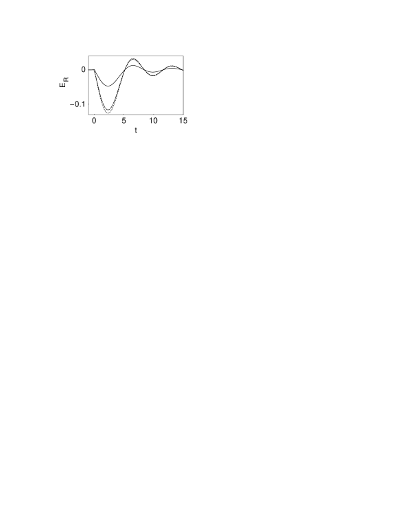
FIG. 2.: Same as in Fig.1, but for an incident pulse of short duration ($\omega_{e}=5$).

The propagation of the reflected pulse in vacuum is characterized by the function $G_{R}(t,x)$, which is the inverse of $\overline{G}_{R}(s,x)$ in (25),

$$G_{R}(t,x)=\delta(t+x).$$ (34)

This means that the reflected pulse $E_{R}(t,x)$ has the space-time dependence $E_{R}(t,x)=E_{R}(t+x)$, and propagates through the vacuum in the negative $x$-direction away from the vacuum-plasma boundary, and without distortion.

We now focus on the transmitted pulse $E_{T}(t,x)$. The propagation of the transmitted pulse through the plasma is characterized by the function $G_{T}(t,x)$ given by the inverse of $\overline{G}_{T}(s,x)$ in (28). $G_{T}(t,x)$ is found by first writing $\overline{G}_{T}(s,x)$ as the spatial derivative

$$\overline{G}_{T}(s,x)=-\partial_{x}\overline{F}_{T}(s,x),$$ (35)

where

$$\overline{F}_{T}(s,x)=\frac{\exp[-(s^{2}+1)^{1/2}x]}{(s^{2}+1)^{1/2}}.$$ (36)

The inverse of $\overline{F}_{T}(s,x)$ is given by [4]

$$F_{T}(t,x)=J_{0}[(t^{2}-x^{2})^{1/2}]H(t-x),$$ (37)

so that

$$G_{T}(t,x) = \delta(t-x)$$ (38)

$$- x\frac{J_{1}[(t^{2}-x^{2})^{1/2}]}{(t^{2}-x^{2})^{1/2}}H(t-x).$$ (39)

Equation (39) represents the combined effect of a distortionless propagation of the transmitted pulse (first term) and the propagation of a dispersive wake generated by the plasma (second term).

We next compute the total Green function $\Gamma_{T}(t,x)$ by inverting (26). One way to do this is to compute $\Gamma_{T}(t,x)$ as the convolution

$$\Gamma_{T}(t,x)=\int_{-\infty}^{\infty}T(t-t^{\prime})G_{T}(t^{\prime},x)\,dt^{\prime},$$ (40)

where $T(t)$ is given by (31), and $G_{T}(t,x)$ by (39). Again, (40) clearly shows the two-stage process of transmission followed by propagation. Analytic evaluation of (40) is quite involved. However, there is a simpler method for obtaining $\Gamma_{T}(t,x)$ analytically that avoids integration, and requires only the computation of derivatives. From (26) and (28), we see that $\overline{\Gamma}_{T}(s,x)$ can be written as the derivative

$$\overline{\Gamma}_{T}(s,x)=-2\partial_{x}[sf(s,x)],$$ (41)

where

$$f(s,x)=\frac{\exp[-(s^{2}+1)^{1/2}x]}{[s+(s^{2}+1)^{1/2}](s^{2}+1)^{1/2}}.$$ (42)

$f(s,x)$ has the inverse transform [4]

$$F(t,x) = {\cal F}(t,x)H(t-x)=\Biggl{(}\frac{t-x}{t+x}\Biggr{)}^{1/2}$$ (43)

$$\times J_{1}[(t^{2}-x^{2})^{1/2}]H(t-x).$$ (44)

This inverse transform only holds for $x>0$, which is in accord with our assumptions of the pulse entering the plasma at $x=0$, and propagating into the plasma for $x>0$. Since $F(0^{+},x)=0$ for $x>0$, we have from standard Laplace transform theory that $\partial_{t}F(t,x)$ is the inverse transform of $sf(s,x)$. Therefore, from (41), we have

$$\Gamma_{T}(t,x)=-2\partial_{tx}^{2}F(t,x).$$ (45)

The term $-2\partial_{tx}^{2}{\cal F}(t,x)$ in (45) represents a modification to the incident pulse, caused by reflection at the vacuum-plasma boundary and dispersion in the plasma. It is given by

$$-2\partial_{tx}^{2}{\cal F}(t,x) = -\frac{xt}{t+x}J_{0}(t^{2}-x^{2})$$ (46)

$$+ \Biggl{(}\frac{xt}{t+x}+\frac{2(t-x)}{(t+x)^{2}}\Biggr{)}$$ (47)

$$\times J_{2}(t^{2}-x^{2}).$$ (48)

From (22), (26), and (28), we see that the transmitted pulse $E_{T}(t,x)$ is given by the Green function integral

$$E_{T}(t,x)=\int_{-\infty}^{\infty}E_{I}(t^{\prime},0)\Gamma_{T}(t-t^{\prime},x)\,dt^{\prime}.$$ (49)

We next perform the integration in (49) for incident pulses of the form (30). We first consider incident pulses of intermediate duration. Figures 3 and 4 show plots of the propagation of ID-HF and ID-IF incident pulses, respectively.

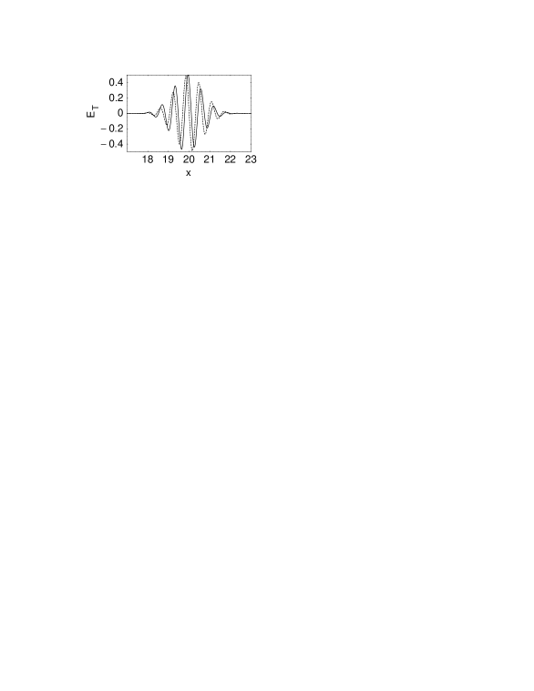
FIG. 3.: Spatial dependence of a transmitted pulse $E_{T}(20,x)$ [Eq. (49)] at time $t=20$ (solid). The incident pulse crossed the vacuum-plasma interface at $t=0$, and had a spatial dependence in vacuum characterized by Eq. (30), $\omega_{e}=1$ (ID), and $\omega_{c}=10$ (HF). The incident pulse’s spatial dependence translated to $t=20$ is shown by the dotted curve, for comparison with the resulting transmitted pulse.

FIG. 4.: Same as in Fig.3, but with incident pulse parameters $\omega_{e}=1$ (ID) and $\omega_{c}=1.5$ (IF).

We see that the high frequency (HF) incident pulse propagates practically undisturbed across the vacuum-plasma interface and into the plasma, while the intermediate-frequency pulse develops an electromagnetic (EM) wake. In the Appendix, we derive the following perturbative expansions for $v_{g}$ and $v_{p}$ in the high-frequency case:

$$v_{g} \approx 1-\epsilon^{2}/2-\epsilon^{4}/8,$$ (50)

$$v_{p}=1/v_{g} \approx 1+\epsilon^{2}/2+3\epsilon^{4}/8,$$ (51)

where $\epsilon=\omega_{p}/\omega_{c}$. The right sides of Eqs. (51) are just the first three terms in the MacLaurin expansions of $(1-\epsilon^{2})^{1/2}$ and $(1-\epsilon^{2})^{-1/2}$.

We next consider the propagation of short (SD) incident pulses. Figure 5 shows a plot of an incident SD-IF pulse.

FIG. 5.: Same as in Fig.3, but with incident pulse parameters $\omega_{e}=5$ (SD) and $\omega_{c}=1.5$ (IF).

As expected, the wake generation is smaller than for the incident ID-IF pulse. And as the frequency of the incident SD pulse is increased, it is found that wake generation is practically nonexistent.

III Summary

In this paper, we considered the transmission and reflection of an electromagnetic pulse at a vacuum-plasma boundary, and the subsequent propagation of the transmitted pulse in the plasma. We extended the well-known theory for long pulses into the short-pulse regime, in which the pulse duration is comparable to the inverse plasma frequency. When the carrier frequency of the incident pulse is much higher than the plasma frequency, most of the incident pulse is transmitted without distortion. Subsequently, the transmitted pulse propagates without distortion at its group speed. When the carrier frequency is comparable to the plasma frequency, the transmitted pulse is distorted, and leaves behind it an electromagnetic wake. The reflected pulse is delayed relative to the incident pulse, and is also distorted. When the carrier frequency is less than the plasma frequency, the incident pulse is absorbed by the plasma before being reemitted.

A Propagation of a high-frequency pulse

Let $\omega_{c}t\rightarrow t$, $\omega_{c}x/c\rightarrow x$, and $\omega_{p}/\omega_{c}\rightarrow\epsilon$, so that $t$ and $x$ become dimensionless. Then the wave equation (1) can be written as

$$\bigl{(}\partial^{2}_{tt}-\partial^{2}_{xx}+\epsilon^{2}\bigr{)}E=0.$$ (A1)

The study of pulse propagation is facilitated by the characteristic transformation

$$\tau=t-\beta x,\ \ \xi=x-\beta t,$$ (A2)

where $\beta<1$. In terms of the characteristic variables $\tau$ and $\xi$, the wave equation (A1) can be rewritten as

$$\bigl{[}(1-\beta^{2})(\partial^{2}_{\tau\tau}-\partial^{2}_{\xi\xi})+\epsilon^{2}\bigr{]}E=0.$$ (A3)

One can solve Eq. (A3) by using multiple scale analysis [5]. To do this, one introduces the time and distance scales

$$\tau_{n}=\epsilon^{n}\tau,\ \ \xi_{n}=\epsilon^{n}\xi.$$ (A4)

Correct to second order, one can write

$$\partial_{\tau} \approx \partial_{\tau_{0}}+\epsilon\partial_{\tau_{1}}+\epsilon^{2}\partial_{\tau_{2}},$$ (A5)

$$\partial_{\xi} \approx \partial_{\xi_{0}}+\epsilon\partial_{\xi_{1}}+\epsilon^{2}\partial_{\xi_{2}}.$$ (A6)

Guided by the well-known characteristics of a long pulse, we assume that

$$\beta\approx 1+\epsilon^{2}\beta_{2}+\epsilon^{4}\beta_{4}$$ (A7)

and

$$E(\tau,\xi)=B(\tau_{2},\xi_{1})\exp(-i\tau_{0}).$$ (A8)

Ansatz (A8) corresponds to a pulse that has a carrier frequency of unity and an amplitude that varies on the slow scale $\xi_{1}$. For this amplitude variation, $\beta$ is the group speed of the pulse, and the characteristic variables are proportional to time and distance measured in the pulse frame. One now substitutes Eqs. (A6) - (A8) in Eq. (A3) and collects terms of like order. The zeroth- and first-order equations are satisfied automatically by construction.

In second order,

$$\bigl{[}-2\beta_{2}(\partial^{2}_{\tau_{0}\tau_{0}}-\partial^{2}_{\xi_{0}\xi_{0}})+1\bigr{]}E=0.$$ (A9)

It follows from Eq. (A9) and ansatz (A8) that

$$\beta_{2}=-1/2.$$ (A10)

In third order,

$$-4\beta_{2}(\partial^{2}_{\tau_{0}\tau_{1}}-\partial^{2}_{\xi_{0}\xi_{1}})E=0.$$ (A11)

Equation (A11) is consistent with ansatz (A8), in which $E$ is assumed to be independent of $\xi_{0}$ and $\tau_{1}$. In fourth order,

$$- \bigl{[}4\beta_{2}(\partial^{2}_{\tau_{0}\tau_{2}}-\partial^{2}_{\xi_{0}\xi_{2}})+2\beta_{2}(\partial^{2}_{\tau_{1}\tau_{1}}-\partial^{2}_{\xi_{1}\xi_{1}})$$ (A12)

$$+ (2\beta_{4}+\beta_{2}^{2})(\partial^{2}_{\tau_{0}\tau_{0}}-\partial^{2}_{\xi_{0}\xi_{0}})\bigr{]}E=0.$$ (A13)

The pulse has a carrier frequency of unity by construction, so the dependence of $E$ on $\tau_{2}$ cannot be oscillatory. It follows from this constraint that $(2\beta_{4}+\beta_{2}^{2})=0$ and, hence, that

$$\beta_{4}=-1/8.$$ (A14)

The group speed $\beta\approx 1-\epsilon^{2}/2-\epsilon^{4}/8$, which is just the first three terms in the Maclaurin expansion of $(1-\epsilon^{2})^{1/2}$. The remaining nonzero terms in Eq. (A13) are

$$\bigl{(}2i\partial_{\tau_{2}}+\partial^{2}_{\xi_{1}\xi_{1}}\bigr{)}B=0,$$ (A15)

which describe the dispersal of the pulse.

Finally, note that ansatz (A8) constrains the phase speed to be the inverse of the group speed. Since no contradictions appear in the subsequent analysis, the assumptions underlying ansatz (A8) are correct. One can also use the ansatz

$$E(\tau,\xi)=B(\tau_{2},\xi_{1})\exp[i\nu\xi_{0}-i(1-\nu\beta)\tau_{0}],$$ (A16)

which does not constrain the phase speed, but leads to the same result.

REFERENCES

- [1] J. D. Jackson, Classical Electrodynamics, 2nd ed. (Wiley, New York, 1975), Chap. 7.
- [2] T. Tajima and J. M. Dawson, Phys. Rev. Lett. 43, 267 (1979).
- [3] P. Sprangle et al., Appl. Phys. Lett. 53, 2146 (1988).
- [4] Handbook of Mathematical Functions, edited by M. Abramowitz and I. E. Stegun (Dover Publications, New York, 1972).
- [5] A. H. Nayfeh, Introduction to Perturbation Techniques (Wiley, New York, 1981).