[

Averaging theory for the structure of hydraulic jumps and separation
in laminar free-surface flows

Abstract

We present a simple viscous theory of free-surface flows in boundary layers, which can accommodate regions of separated flow. In particular this yields the structure of stationary hydraulic jumps, both in their circular and linear versions, as well as structures moving with a constant speed. Finally we show how the fundamental hydraulic concepts of subcritical and supercritical flow, originating from inviscid theory, emerge at intermediate length scales in our model.

]

Despite the classical nature of the subject, the flow of a viscous fluid with a free surface presents many unsolved theoretical problems, even under laminar conditions. To a large extent this is due to the lack of approximate methods for describing flows containing separated regions, i.e. regions in which the flow is reversed with respect to the mean flow. Hydraulic jumps are examples of such flows. They are large, sudden deformations in the free surface of stationary flows [1] and no theory exists for their structure — save the full Navier-Stokes equations combined with the free-surface boundary conditions, for which even numerical solution poses large problems. In this Letter we present a method for determining some of these flows, which includes viscosity and variations of the velocity profile. Stationary states are obtained as trajectories in a simple two-dimensional phase space.

An inviscid theory of hydraulic jumps, which is still the standard hydraulic approach to the subject, is due to Lord Rayleigh in 1914 [2, 3]. He regarded hydraulic jumps as discontinuities (shocks) which can occur in the shallow water equations [4]. Across a jump the flow decelerates from a rapid supercritical flow, in which disturbances propagate only down stream, to a subcritical flow, in which they propagate in both directions.

The circular hydraulic jump is easy to study experimentally and to maintain in a laminar state. Here a jet of fluid falls vertically onto a horizontal surface (Fig. 1). The fluid spreads in an axisymmetric way, and a hydraulic jump is formed at some $r_{j}$. The value of $r_{j}$ cannot be found by the standard theory, and it depends strongly on viscosity $\nu$ [5]. Further, experiments show clearly that a separation bubble, or a recirculating region, forms on the bottom in conjunction with the jump [5, 6, 7, 8].

Separation per se has been studied more intensely in boundary layers close to solid bodies, e.g. airfoils, immersed in a high Reynolds number flow. This line of research descends from Prandtl’s seminal work [9] in which he introduced the boundary layer approximation — a radical simplification of the Navier-Stokes equations. Prandtl’s equations are valid in a thin layer near solid (no-slip) surfaces, where the fluid motion is predominantly along the surface. But in general, they become singular at separation points [10], where the assumption of forward flow breaks down. The boundary layer equations can be further simplified by using an averaging technique of von Karman and Pohlhausen [9], in which the tangential velocity profile is approximated as a low order polynomium. This model is useful up to a separation point, but solutions beyond the point tend to diverge and are discarded. Such troubles can be cured by taking into account the feed-back effect from the boundary layer on the external flow. The “inverse method” [11] makes it possible to calculate flows with separation bubbles, and analytical results have been obtained for the structure of separation points at large Reynolds numbers [12].

It is natural to employ the boundary layer approximation to describe hydraulic jumps since the fluid moves nearly parallel to the bottom surface. To avoid the singularities near a jump encountered in earlier work [6, 5] we use the Karman-Pohlhausen method. The standard hydrostatic approximation then provides the link between pressure and layer thickness analogous to the feedback mechanism in the inverse method used above [13].

For a stationary, radially symmetric flow with a free surface the boundary layer equations take the form

$$uu_{r}+wu_{z}=-gh^{\prime}+\nu u_{zz}$$ (1)

$$u_{r}+u/r+w_{z}=0$$ (2)

where $u(r,z)$ and $w(r,z)$ are the radial ($r$) and vertical ($z$) velocity components, $h(r)$ is the height, and we assume hydrostatic pressure. Surface tension has been neglected, since it does not appear to be decisive in determining the structure of the flow, although it is necessary for the stability of the flows as discussed below. The boundary conditions are no-slip on the bottom: $u(r,0)=w(r,0)=0$, no stress on the top: $u_{z}(r,h)=0$ (strictly valid only for small deformations $|h^{\prime}|$) and the kinematic boundary condition at the top: $w(r,h)=u(r,h)h^{\prime}$, which ensures the mass conservation: $2\pi r\int_{0}^{h}udz=$const.$=Q=2\pi q$. By rescaling the horizontal and vertical lengths and velocities by $L=(q^{5}\nu^{-3}g^{-1})^{1/8}$, $H=(q\nu g^{-1})^{1/4}$, and $V=(q\nu g^{3})^{1/8}$, respectively, all parameters are eliminated from (1,2) [5].

We average these equations over $z$, but in contrast to earlier approaches [6, 5] we shall not assume a self-similar velocity profile. Instead the velocity profile is parametrized as

$$u(r,z)=v(r)\left(a_{1}(r)\eta+a_{2}(r)\eta^{2}+a_{3}(r)\eta^{3}\right)$$ (3)

where $\eta=z/h(r)$. Implementing the boundary conditions reduces the parameters to just one: $\lambda(r)$, i.e. $a_{1}=\lambda+3$, $a_{2}=-(5\lambda+3)/2$ and $a_{3}=4\lambda/3$. Thus the profile is parabolic when $\lambda=0$ and separation occurs for $\lambda=-3$. With these assumptions the averaged momentum equation (1) takes the form [13]

$$v(F_{2}(\lambda)v)^{\prime}=-h^{\prime}-(\lambda+3)v/h^{2}$$ (4)

where $F_{2}(\lambda)=(\int_{0}^{h}u^{2}dz)/(hv^{2})=6/5-\lambda/15+\lambda^{2}/105$ and $rhv=1$. To determine $\lambda$, one more equation is needed, and this is (as in the standard Karman-Pohlhausen approach [9]) taken to be (1) evaluated on the bottom ($z=0$), which gives

$$h^{\prime}=-(5\lambda+3)v/h^{2}.$$ (5)

When $v=1/(rh)$ is inserted into (4,5) we obtain a non-autonomous flow for the two-dimensional vector field $(h,\lambda)$. The flow has singularities only on the lines $h=0$ and $\lambda=7/2$. It is thus possible to obtain both separation and parabolic profiles without crossing singularities.

We solve the system with two boundary conditions. Since the velocity profiles are not measured, we impose two surface points $h_{1}(r_{1})$ and $h_{2}(r_{2})$, read from a recent measurement of Ellegaard et al. [8]. Iterative adjustment of $\lambda$ at one end converges to a solution which passes through the two chosen points. Figure 2(a) shows comparison of the calculated height $h(r)$ and the measurements, for two different $h_{2}$ values. The surface profiles near $r_{j}$ show fair agreements, considering the simplicity of the model, but $r_{j}$ is off by around 15%. Figure 2(b) shows the calculated $\lambda(r)$. A separation zone ($\lambda<-3$) occurs just behind the jump and its size increases as $h_{2}$ is raised, just as observed. The streamlines and velocity profiles are determined from $\lambda$, and this leads to a graphical representation of the flow as shown in Fig. 1(b).

The model captures the experimental feature that $h(r)$ inside the jump is little affected by the change in $h_{2}$. The curves in Fig. 2(a) apparently follow a single curve inside the jump, from which trajectories diverge when $r$ is increased. Backward integration from $r_{2}$ automatically settles down to this value of $\lambda$, which helps us since the entrance velocity profile need not be specified. Further details of the phase space structure can be found in [13].

Another quantity measured in [8] is the surface velocity $U(r)=u(r,h(r))$. Comparison is made in Fig. 3, which shows quantitative agreement, although $r_{j}$ again comes out smaller. There is no free parameter other than $h_{1,2}$, taken from the experiments.

One can apply these methods to time-dependent flows. Since the time-dependent circular jumps typically involve breaking of the radial symmetry [8], we take, as an example, the two-dimensional (Cartesian) flow down an inclined plane. There exists a large body of literature [14, 15, 16, 17] on such flows to which we shall be able to compare. We non-dimensionalize in terms of the parabolic laminar solution [17] with a constant height $h_{0}$, mean velocity $v_{0}$, and flux $q_{0}$ related by $q_{0}=h_{0}v_{0}=gh_{0}^{3}\sin\alpha/(3\nu)$, where $\alpha$ is the bottom slope. The Reynold number is $R=v_{0}h_{0}/\nu=q_{0}/\nu$ while the Froude number is $F=v_{0}^{2}/(gh_{0}\cos\alpha)=R\tan\alpha/3$. We obtain [13]

$$h_{t}+(hv)_{x}=0$$ (6)

$$\frac{R}{3h}\left[(hv)_{t}+(hv^{2}F_{2}(\lambda))_{x}\right]+h_{x}\cot\alpha$$ (7)

$$=1-(\lambda+3)v/(3h^{2})$$ (8)

$$h_{x}\cot\alpha=1-(5\lambda+3)v/(3h^{2})$$ (9)

where $x$ is the scaled downward distance along the plane.

We first study stationary solutions to the equations. Then, $hv=1$ from (6), and (8,9) form an autonomous two-dimensional system for $(\lambda,h)$, that can be easily studied on a phase portrait. (This is the Cartesian version of (4,5).) There is a unique fixed point $h=1$ and $\lambda=0$, and thus one cannot find stationary states connecting two different states with constant $(h,\lambda)$. (This can, however, be done for traveling waves; see below.) On the other hand an interesting solution [18] is represented by the stable manifold of the fixed point emerging from $h=0$ as shown in Fig. 4. The first part of the trajectory has $h_{x}$ nearly constant [19], i.e. $h\approx A(x-x_{0})/R$ and $\lambda\approx-3/5$ until it suddenly jumps up to the fixed point values. Inserting into (6,8), we get $A=2.4/F_{2}(-3/5)\approx 1.93$. We believe this represents flows that are observed behind sluice gates though we treat the flow as laminar [20]. The conventional hydraulic theory predicts [3] that a jump occurs behind a gate when the bottom slope is “mild” (i.e. $\alpha$ being less than a critical slope). Correspondingly, the jump structure in Fig. 4 disappears as $R\tan\alpha=3F$ is increased beyond $A$ [13].

It is also possible to find a traveling wave solution [16] which connects two parabolic laminar solutions of height $h_{1}$ at $x=-\infty$ and $h_{2}$ at $x=\infty$ [21]. These two limits thus carry different fluxes, such that the flux is conserved in the moving frame only. By choosing the characteristic height appropriately, we may set $h_{1}h_{2}=1$ without loss of generality. Then we define the moving frame by $\xi=x-ct$, and look for a stationary solutions in $\xi$, which by (6) must satisfy $c=h_{1}^{2}+h_{1}h_{2}+h_{2}^{2}(>3)$. There are two fixed points $h=h_{1,2}$, both with $\lambda=0$, and a heteroclinic solution from $h_{1}$ to $h_{2}(<h_{1})$ as $\xi$ increases can be found [13] iff $R\tan\alpha<60h_{1}^{3}/(25c^{2}h_{1}^{4}-61ch_{1}^{2}+33)$. Such river-bore like solutions are calculated and shown in Fig. 5 for a fixed $h_{1}$ and $\alpha$ and varying $R$. Note that the velocity profile always remains near parabolic as $\lambda$ departs only slightly from zero, and that the width of the “shock” is much larger than the thickness of the layer, unlike the steady jump (Fig. 4).

Finally, we study the dispersion of small disturbances in the time-dependent system. The spectrum of the uniform state ($h=v=1$, $\lambda=0$) allows the distinction between super- and subcritical flows, which is fundamental to hydraulics but not obvious for viscous flows. Surface tension is necessary for the stability calculations. An additional term $(+RWh_{xxx}/3)$ thus appears on the right hand sides of (8,9), where $W=\sigma/(\rho h_{0}v_{0}^{2})=9\sigma\nu^{2}/(\rho gh_{0}^{5}\sin^{2}\alpha)$ is the Weber number.

Assuming that all disturbances vary like $\exp(ikx-i\omega t)$, we obtain [13] two dispersion branches. In the $k\rightarrow 0$ limit they behave as $\omega_{+}(k)\sim 3k+ik^{2}(5R/4-\cot\alpha)+O(k^{3})$ and $\omega_{-}(k)\sim-14k/25-12i/5R+O(k^{3})$. Thus, the $\omega_{-}$ branch moves backwards, and the flow is, irrespective of the Froude number, “subcritical”. From the imaginary parts, both branches are stable for a small $R$, but the $\omega_{+}$ branch becomes unstable for $R\tan\alpha>4/5$. This is in qualitative agreement with other models, notably those coming from perturbation expansions [15, 16, 22] and from averaging [17]. The so-called “Shkadov model” [17] is identical to our system (6,8) with a rigid parabolic profile, i.e. $\lambda\equiv 0$, and omitting (9).

For very large $k$ the model shows unphysical behavior, as one branch becomes unstable. A priori we have no reason to expect our model to be well defined at length scales much smaller than the normalized height, since our starting point is the boundary layer approximation. High-frequency oscillations are expected not to penetrate far into the fluid, but our assumption of the hydrostatic pressure still connects $\lambda$ and $h$ rigidly. We can remedy this by modifying (9), such that $\lambda$ depends on a spatial average of $h$ and $h_{x}$ over an interval of the order of a fraction of $h$ [23]. In this way, the limit $k\rightarrow\infty$ now corresponds to the Shkadov model [17] and is stable.

For intermediate $k$, the dispersion behavior is very interesting. When $R\tan\alpha>20/11\approx 1.82$, the group velocity of both branches will have positive real parts, and the flow is “supercritical”. In terms of the Froude number, this inequality becomes $F>20/33$ which is similar to the classical criterion of $F>1$ even though our theory includes viscosity. For large $R\tan\alpha$, the subcritical range of $k$ is so small that this supercritical behavior dominates. In Fig. 6, we show dispersion curves (the real parts of $\omega_{\pm}$) for $R=25$, $\alpha=5$ [deg], and $W=0.01$. The slope of the $\omega_{+}$ branch is always positive. On the other hand, the slope of the $\omega_{-}$ branch changes its sign. The subcritical small-$k$ region is small, and such long-wave disturbances become hard to create. Note that the criterion $R\tan\alpha=3F<A\approx 1.93$ for the existence of a stationary jump (Fig. 4) is almost equivalent to the demand that the final state $h=1$ be subcritical ($R\tan\alpha<1.82$). On the other hand, the linearly increasing part before the jump in Fig. 4 is expected to be supercritical, but the dispersion around the solution is hard to obtain due to its finite extent and the non-uniform character. In contrast, for the moving jumps in Fig. 5, super- or sub-criticality must be determined with respect to the jump. It can be shown [13] that the flow is supercritical in front of the jump and subcritical behind, as expected.

To conclude, we have presented a simple model of free-surface flows which can describe separation and the structure of the circular and linear hydraulic jumps.

We thank Clive Ellegaard, Adam E. Hansen and Anders Haaning for many discussions and for providing us with experimental data. We would also like to thank Ken H. Andersen, Peter Dimon, Lisbeth Kjeldgaard and Hiraku Nishimori for stimulating discussions.

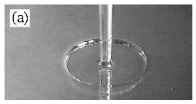
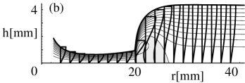
FIG. 1.: (a) A circular hydraulic jump is formed when a liquid jet falls onto a plate from above (photo: courtesy of A. E. Hansen). (b) Surface profile, streamlines, and the horizontal velocity profile in a cross section, predicted from our model (see text and Fig. 2). Note the difference in the scales for the two axes. The profile is nearly parabolic at large radius, but is strongly deformed near the jump. The shaded area is a separation bubble.

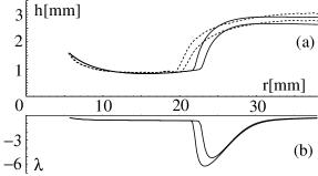
FIG. 2.: (a) Measured $h(r)$ (dashed curves) vs. our model (solid curves). The model uses a shooting method from $r_{2}=30$[mm] toward $r_{1}=12$[mm] for a fixed inner height $h_{1}$ and two outer heights $h_{2}$. Fluid: 50% ethylene glycol ($Q=27$[m$\ell$/s], $\nu=7.6\times 10^{-6}$[m²/s]). Length and velocity scales: $L=28$[mm], $H=1.4$[mm], and $V=12$[cm/s]. (b) The model predicts a larger separation zone as $h_{2}$ increases.

FIG. 3.: Measured surface velocity $U(r)$ (dots) vs. our model (dotted lines). Parameters: 80% ethylene glycol ($Q=34$[m$\ell$/s], $\nu=14.4\times 10^{-6}$[m²/s]), $L=25$[mm], $H=1.7$[mm], and $V=16$[cm/s]. The jump is located at $r_{j}\approx 24$[mm] (experiment) and 20[mm] (model). The inset is an enlargement at large $r$ in a log–log scale.

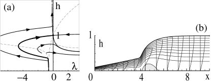
FIG. 4.: Stationary solutions to the inclined plane equations (6–9) with $R=30$ and $\alpha=1$[deg]. Phase portrait (a) has a saddle fixed point at $(h,\lambda)=(1,0)$. Dashed curves are nullclines $h^{\prime}=0$ or $\lambda^{\prime}=0$. Among trajectories (solid curves), one stable manifold (drawn thicker) to the saddle point corresponds to the hydraulic jump solution shown in (b).

FIG. 5.: Traveling wave solutions to the inclined plane equations. $h_{1}=1/h_{2}=5/4$, $\alpha=2$[deg], and $R=3,7,9.4$. The $u$-profile stays near parabolic ($\lambda=0$). Oscillation starts when $R\tan\alpha$ is near a critical value.

FIG. 6.: Real part of the dispersion relation $\omega(k)$.

REFERENCES

- [1] Similar moving structures are usually called river bores.
- [2] Lord Rayleigh, Proc. Roy. Soc. A, 90, 324 (1914).
- [3] V. T. Chow, Open channel hydraulics, (McGraw Hill, 1973). M. Manohar & P. Krishnamachar, Fluid Mechanics 1 (Vikas, Delhi, 1994). J. M. Townson, Free-surface hydraulics, (Unwin Hyman, 1991).
- [4] G. B. Whitham, Linear & Nonlinear Waves, (Wiley-Interscience, 1974).
- [5] T. Bohr, P. Dimon & V. Putkaradze, J. Fluid Mech., 254, 635 (1993).
- [6] I. Tani, J. Phys. Soc. Japan, 4, 212 (1949).
- [7] A. Craik et al., J. Fluid Mech. 112, 347 (1981); R. Bowles & F. Smith, J. Fluid. Mech, 242, 145 (1992).
- [8] C. Ellegaard et al., Phys. Scr., T67, 105 (1996). In the present article we have concentrated on the “type 1” flow in the terminology of this reference.
- [9] H. Schlichting, Boundary Layer Theory, (McGraw Hill, 1968).
- [10] S. Goldstein, Q. J. Mech. Appl. Math., 1, 43 (1948); L. D. Landau & E. M. Lifschitz, Fluid Mechanics, (Pergamon, 1959).
- [11] D. Catherall & K. Mangler, J. Fluid Mech., 26, 163 (1966); A. E. P. Veldman, AIAA J., 19, 79 (1981).
- [12] F. Smith, Ann. Rev. Fluid Mech., 18, 197 (1986).
- [13] S. Watanabe, V. Putkaradze & T. Bohr, unpublished.
- [14] P. L. Kapitza & S. P. Kapitza in Collected works by P. L. Kapitza, p. 690 (Pergamon, 1965).
- [15] D. J. Benney, J. Maths & Phys., 45, 150 (1966); C. Nakaya, Phys. Fluids, 18, 1407 (1975).
- [16] A. Pumir, P. Manneville & Y. Pomeau, J. Fluid Mech., 135, 27 (1983).
- [17] H.-C. Chang, J. Fluid Mech., 250, 433 (1993); Ann. Rev. Fluid Mech., 26, 103 (1993).
- [18] A similar flow has been found in numerical solution of the boundary layer equation in F. Higuera, J. Fluid. Mech, 274, 69 (1994).
- [19] This conforms with E. J. Watson, J. Fluid Mech., 20, 481 (1964). We obtain similar agreement in the radial case [13].
- [20] It is presumably possible to replace the loss term in (6-9) to model turbulent flows, as e.g. in [4].
- [21] It is also possible to study homoclinic orbits [16, 17], but there surface tension appears crucial.
- [22] The model used in [16] has only one branch of dispersion relation and thus no distinction between supercritical and subcritical flow.
- [23] The modified equation (9) is where and . In the limit this reduces to (9) and signifies the cutoff in , which, in Fig. 6 was .