Incorporation of the statistical uncertainty in the background estimate into the upper limit on the signal

Abstract

We present a procedure for calculating an upper limit on the number of signal events which incorporates the Poisson uncertainty in the background, estimated from control regions of one or two dimensions. For small number of signal events, the upper limit obtained is more stringent than that extracted without including the Poisson uncertainty. This trend continues until the number of background events is comparable with the signal. When the number of background events is comparable or larger than the signal, the upper limit obtained is less stringent than that extracted without including the Poisson uncertainty. It is therefore important to incorporate the Poisson uncertainty into the upper limit; otherwise the upper limit obtained could be too stringent.

OHSTPY-HEP-E-97-009

1 Introduction

In the search for a rare or forbidden process, an experiment usually observes zero or few candidate events and sets an upper limit on the number of signal events. The background is often estimated from control regions of one or two dimensions. In the case of a small number of candidates events, it is important to incorporate the uncertainty in the background estimate due to Poisson statistics into the upper limit.

For $N_{ob}$ observed events with an expected background of $N_{bg}$ events, the upper limit on the number of signal events $\lambda_{0}$ at a confidence level $\delta$ is given by:

$$\frac{e^{-(\lambda_{0}+N_{bg})}\sum_{n=0}^{N_{ob}}\frac{(\lambda_{0}+N_{bg})^{n}}{n!}}{e^{-N_{bg}}\sum_{n=0}^{N_{ob}}\frac{(N_{bg})^{n}}{n!}}=1-\delta,$$ (1)

assuming that there is no uncertainty in the background estimate [1, 2]. In this paper, we present a procedure for incorporating the statistical uncertainty in the background estimate using Poisson statistics.

2 Incorporation of the statistical uncertainty

We consider the case in which the background is estimated from control regions of one or two dimensions which have limited statistics. Figure 1(a) shows an example of a signal and two sideband regions in the distribution of a physical variable for the one-dimensional case. The corresponding example for the two-dimensional case for the signal, four sideband and four corner-band regions is shown in Fig. 1(b). Assuming that the background is linear in the vicinity of the signal region, the background in the signal region can be estimated from the number of events in the sideband (and corner-band if appropriate) regions. The number of signal events $N_{0}$ is given by:

$$N_{0}=N_{ob}-N_{bg}\equiv N_{ob}-\alpha N_{sb}+\beta N_{cb},$$ (2)

where $N_{sb}$ ($N_{cb}$) is the number of events in the sideband (corner-band) regions. For the one-dimensional case, $\alpha$ is the ratio of the width of the signal region to the total width of the sideband regions and $\beta$ is zero. In the two-dimensional case, $\alpha$ is two times the ratio of the area of the signal region to the total area of the sideband regions and $\beta$ is the ratio of the area of the signal region to the total area of the corner-band regions.

     

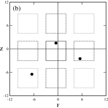
Figure 1: (a) Definition of signal and two sideband regions (arrowed brackets) in the $X$ distribution for the one-dimensional case. The width of the sideband regions is the same as the signal region. (b) Definition of signal, sideband (dashed), and corner-band (dotted) regions in the $Y$ vs. $Z$ distribution for the two-dimensional case. The area of a sideband or corner-band region is the same as the signal region.

The extraction of the upper limit on the signal must account for the uncertainty in the background estimate due to limited statistics in the control regions. For the one-dimensional case, this is implemented by expanding Eq. (1) to sum over all possible background values weighted by the Poisson probability for observing the $N_{sb}$ background events given an expected number of events $\lambda_{sb}$ in the sideband regions. The upper limit on the number of signal events $\lambda$ at a confidence level $\delta$ is given by:

$$\frac{\int_{0}^{\infty}d\lambda_{sb}\frac{\lambda_{sb}^{N_{sb}}}{N_{sb}!}e^{-\lambda_{sb}}e^{-(\lambda+\alpha\lambda_{sb})}\sum_{n=0}^{N_{ob}}\frac{(\lambda+\alpha\lambda_{sb})^{n}}{n!}}{\int_{0}^{\infty}d\lambda_{sb}\frac{\lambda_{sb}^{N_{sb}}}{N_{sb}!}e^{-\lambda_{sb}}e^{-\alpha\lambda_{sb}}\sum_{n=0}^{N_{ob}}\frac{(\alpha\lambda_{sb})^{n}}{n!}}$$ (3)

$$= \frac{\sum_{n=0}^{N_{ob}}\sum_{k=0}^{n}\frac{\alpha^{k}\lambda^{n-k}e^{-\lambda}(N_{sb}+k)!}{(1+\alpha)^{k}k!(n-k)!}}{\sum_{k=0}^{N_{ob}}\frac{\alpha^{k}(N_{sb}+k)!}{(1+\alpha)^{k}k!}}$$

$$= 1-\delta.$$

The integral of $\lambda_{sb}$ is performed with $\int_{0}^{\infty}dye^{-y}y^{k}=k!$. Note that this formula can also be used to calculate the upper limit on the number of signal events for the case in which the background is estimated from a Monte Carlo simulation. In this case, $N_{sb}$ is the number of background events that satisfied the event selection criteria in a Monte Carlo sample that is $\alpha^{-1}$ times larger than the data.

For control regions of two dimensions, the formula for the upper limit is much more complicated. However, it can be simplified depending on the value of $\beta$. In the case of $\beta=1$ which corresponds a total corner-band area that is equal to the area of the signal region, the upper limit is given by:

$$\frac{\int_{0}^{\infty}d\lambda_{sb}\int_{0}^{\alpha\lambda_{sb}}d\lambda_{cb}\frac{\lambda_{sb}^{N_{sb}}}{N_{sb}!}e^{-\lambda_{sb}}\frac{\lambda_{cb}^{N_{cb}}}{N_{cb}!}e^{-\lambda_{cb}}e^{-(\lambda+\alpha\lambda_{sb}-\lambda_{cb})}\sum_{n=0}^{N_{ob}}\frac{(\lambda+\alpha\lambda_{sb}-\lambda_{cb})^{n}}{n!}}{\int_{0}^{\infty}d\lambda_{sb}\int_{0}^{\alpha\lambda_{sb}}d\lambda_{cb}\frac{\lambda_{sb}^{N_{sb}}}{N_{sb}!}e^{-\lambda_{sb}}\frac{\lambda_{cb}^{N_{cb}}}{N_{cb}!}e^{-\lambda_{cb}}e^{-(\alpha\lambda_{sb}-\lambda_{cb})}\sum_{n=0}^{N_{ob}}\frac{(\alpha\lambda_{sb}-\lambda_{cb})^{n}}{n!}}$$ (4)

$$= \frac{\sum_{n=0}^{N_{ob}}\sum_{k=0}^{n}\frac{\alpha^{k}\lambda^{n-k}e^{-\lambda}}{(1+\alpha)^{k}(n-k)!}\sum_{j=0}^{k}\frac{(-1)^{k-j}(N_{sb}+N_{cb}+k+1)!}{j!(k-j)!(N_{cb}+k-j+1)}}{\sum_{k=0}^{N_{ob}}\frac{\alpha^{k}}{(1+\alpha)^{k}}\sum_{j=0}^{k}\frac{(-1)^{k-j}(N_{sb}+N_{cb}+k+1)!}{j!(k-j)!(N_{cb}+k-j+1)}}$$

$$= 1-\delta,$$

where $\lambda_{cb}$ is the expected number of events in the corner-band regions. Note that the unphysical region ($\lambda_{cb}>\alpha\lambda_{sb}$) is excluded from the integral.

For a larger corner-band area, $0<\beta<1$, the upper limit is given by:

$$\frac{\int_{0}^{\infty}d\lambda_{sb}\int_{0}^{\gamma\lambda_{sb}}d\lambda_{cb}\frac{\lambda_{sb}^{N_{sb}}}{N_{sb}!}e^{-\lambda_{sb}}\frac{\lambda_{cb}^{N_{cb}}}{N_{cb}!}e^{-\lambda_{cb}}e^{-(\lambda+\alpha\lambda_{sb}-\beta\lambda_{cb})}\sum_{n=0}^{N_{ob}}\frac{(\lambda+\alpha\lambda_{sb}-\beta\lambda_{cb})^{n}}{n!}}{\int_{0}^{\infty}d\lambda_{sb}\int_{0}^{\gamma\lambda_{sb}}d\lambda_{cb}\frac{\lambda_{sb}^{N_{sb}}}{N_{sb}!}e^{-\lambda_{sb}}\frac{\lambda_{cb}^{N_{cb}}}{N_{cb}!}e^{-\lambda_{cb}}e^{-(\alpha\lambda_{sb}-\beta\lambda_{cb})}\sum_{n=0}^{N_{ob}}\frac{(\alpha\lambda_{sb}-\beta\lambda_{cb})^{n}}{n!}}$$ (5)

$$= \frac{\sum_{n=0}^{N_{ob}}\sum_{k=0}^{n}\alpha^{k}\frac{\lambda^{n-k}e^{-\lambda}}{(n-k)!}\sum_{j=0}^{k}\frac{(-1)^{k-j}(N_{cb}+k-j)!}{(\gamma-\alpha)^{k-j}j!(k-j)!}\left[\frac{(N_{sb}+j)!}{(1+\alpha)^{N_{sb}+j+1}}-\sum_{i=0}^{N_{cb}+k-j}\frac{(\gamma-\alpha)^{i}(N_{sb}+j+i)!}{(1+\gamma)^{N_{sb}+j+i+1}i!}\right]}{\sum_{k=0}^{N_{ob}}\alpha^{k}\sum_{j=0}^{k}\frac{(-1)^{k-j}(N_{cb}+k-j)!}{(\gamma-\alpha)^{k-j}j!(k-j)!}\left[\frac{(N_{sb}+j)!}{(1+\alpha)^{N_{sb}+j+1}}-\sum_{i=0}^{N_{cb}+k-j}\frac{(\gamma-\alpha)^{i}(N_{sb}+j+i)!}{(1+\gamma)^{N_{sb}+j+i+1}i!}\right]}$$

$$= 1-\delta,$$

where the unphysical region ($\lambda_{cb}>\frac{\alpha}{\beta}\lambda_{sb}\equiv\gamma\lambda_{sb}$) is excluded from the integral. The integral of $\lambda_{cb}$ is obtained with $\int_{0}^{x}dye^{-y}y^{k}=k!(1-\sum_{i=0}^{k}\frac{x^{i}}{i!}e^{-x})$.

In the following sections, we consider two widely used relative dimensions between the signal and control regions.

2.1 Case I: $\alpha=\frac{1}{2}$ and $\beta=\frac{1}{4}$

We first consider the one-dimensional case in which the total width of the sideband regions is twice that of the signal region as shown in Fig. 1(a). This corresponds to $\alpha=\frac{1}{2}$ and Eq. (3) for the upper limit on the signal is simplified to:

$$\frac{\int_{0}^{\infty}d\lambda_{sb}\frac{\lambda_{sb}^{N_{sb}}}{N_{sb}!}e^{-\lambda_{sb}}e^{-(\lambda+\frac{\lambda_{sb}}{2})}\sum_{n=0}^{N_{ob}}\frac{(\lambda+\frac{\lambda_{sb}}{2})^{n}}{n!}}{\int_{0}^{\infty}d\lambda_{sb}\frac{\lambda_{sb}^{N_{sb}}}{N_{sb}!}e^{-\lambda_{sb}}e^{-\frac{\lambda_{sb}}{2}}\sum_{n=0}^{N_{ob}}\frac{(\frac{\lambda_{sb}}{2})^{n}}{n!}}$$ (6)

$$= \frac{\sum_{n=0}^{N_{ob}}\sum_{k=0}^{n}\frac{\lambda^{n-k}e^{-\lambda}(N_{sb}+k)!}{3^{k}k!(n-k)!}}{\sum_{k=0}^{N_{ob}}\frac{(N_{sb}+k)!}{3^{k}k!}}$$

$$= 1-\delta.$$

We now consider the two-dimensional case in which the total area of both the sideband and corner-band regions is four times that of the signal region as shown in Fig. 1(b). This corresponds to $\alpha=\frac{1}{2}$ and $\beta=\frac{1}{4}$. From Eq. (5), the upper limit on the signal is given by:

$$\frac{\int_{0}^{\infty}d\lambda_{sb}\int_{0}^{2\lambda_{sb}}d\lambda_{cb}\frac{\lambda_{sb}^{N_{sb}}}{N_{sb}!}e^{-\lambda_{sb}}\frac{\lambda_{cb}^{N_{cb}}}{N_{cb}!}e^{-\lambda_{cb}}e^{-(\lambda+\frac{\lambda_{sb}}{2}-\frac{\lambda_{cb}}{4})}\sum_{n=0}^{N_{ob}}\frac{(\lambda+\frac{\lambda_{sb}}{2}-\frac{\lambda_{cb}}{4})^{n}}{n!}}{\int_{0}^{\infty}d\lambda_{sb}\int_{0}^{2\lambda_{sb}}d\lambda_{cb}\frac{\lambda_{sb}^{N_{sb}}}{N_{sb}!}e^{-\lambda_{sb}}\frac{\lambda_{cb}^{N_{cb}}}{N_{cb}!}e^{-\lambda_{cb}}e^{-(\frac{\lambda_{sb}}{2}-\frac{\lambda_{cb}}{4})}\sum_{n=0}^{N_{ob}}\frac{(\frac{\lambda_{sb}}{2}-\frac{\lambda_{cb}}{4})^{n}}{n!}}$$ (7)

$$= \frac{\sum_{n=0}^{N_{ob}}\sum_{k=0}^{n}\frac{\lambda^{n-k}e^{-\lambda}}{3^{k}(n-k)!}\sum_{j=0}^{k}\frac{(-1)^{k-j}(N_{cb}+k-j)!}{j!(k-j)!}[(N_{sb}+j)!-\sum_{i=0}^{N_{cb}+k-j}\frac{(N_{sb}+j+i)!}{2^{N_{sb}+j+i+1}i!}]}{\sum_{k=0}^{N_{ob}}\frac{1}{3^{k}}\sum_{j=0}^{k}\frac{(-1)^{k-j}(N_{cb}+k-j)!}{j!(k-j)!}[(N_{sb}+j)!-\sum_{i=0}^{N_{cb}+k-j}\frac{(N_{sb}+j+i)!}{2^{N_{sb}+j+i+1}i!}]}$$

$$= 1-\delta.$$

2.2 Case II: $\alpha=\beta=1$

We first consider the one-dimensional case in which the total width of the sideband regions is the same as that of the signal region (Fig. 2(a)); an experimenter may choose this kind of smaller background control regions so that the background is more linear in the vicinity of the signal region. Substituting for $\alpha=1$ in Eq. (3), the upper limit of the signal is given by:

$$\frac{\int_{0}^{\infty}d\lambda_{sb}\frac{\lambda_{sb}^{N_{sb}}}{N_{sb}!}e^{-\lambda_{sb}}e^{-(\lambda+\lambda_{sb})}\sum_{n=0}^{N_{ob}}\frac{(\lambda+\lambda_{sb})^{n}}{n!}}{\int_{0}^{\infty}d\lambda_{sb}\frac{\lambda_{sb}^{N_{sb}}}{N_{sb}!}e^{-\lambda_{sb}}e^{-\lambda_{sb}}\sum_{n=0}^{N_{ob}}\frac{(\lambda_{sb})^{n}}{n!}}$$ (8)

$$= \frac{\sum_{n=0}^{N_{ob}}\sum_{k=0}^{n}\frac{\lambda^{n-k}e^{-\lambda}(N_{sb}+k)!}{2^{k}k!(n-k)!}}{\sum_{k=0}^{N_{ob}}\frac{(N_{sb}+k)!}{2^{k}k!}}$$

$$= 1-\delta.$$

We now consider the two-dimensional case in which the total area of the sideband regions is twice that of the signal region and the total area of corner-band regions is the same as that of the signal region (Fig. 2(b)). The upper limit is given by Eq. (4) through substitution of $\alpha=\beta=1$:

$$\frac{\int_{0}^{\infty}d\lambda_{sb}\int_{0}^{\lambda_{sb}}d\lambda_{cb}\frac{\lambda_{sb}^{N_{sb}}}{N_{sb}!}e^{-\lambda_{sb}}\frac{\lambda_{cb}^{N_{cb}}}{N_{cb}!}e^{-\lambda_{cb}}e^{-(\lambda+\lambda_{sb}-\lambda_{cb})}\sum_{n=0}^{N_{ob}}\frac{(\lambda+\lambda_{sb}-\lambda_{cb})^{n}}{n!}}{\int_{0}^{\infty}d\lambda_{sb}\int_{0}^{\lambda_{sb}}d\lambda_{cb}\frac{\lambda_{sb}^{N_{sb}}}{N_{sb}!}e^{-\lambda_{sb}}\frac{\lambda_{cb}^{N_{cb}}}{N_{cb}!}e^{-\lambda_{cb}}e^{-(\lambda_{sb}-\lambda_{cb})}\sum_{n=0}^{N_{ob}}\frac{(\lambda_{sb}-\lambda_{cb})^{n}}{n!}}$$ (9)

$$= \frac{\sum_{n=0}^{N_{ob}}\sum_{k=0}^{n}\frac{\lambda^{n-k}e^{-\lambda}}{2^{k}(n-k)!}\sum_{j=0}^{k}\frac{(-1)^{k-j}(N_{sb}+N_{cb}+k+1)!}{j!(k-j)!(N_{cb}+k-j+1)}}{\sum_{k=0}^{N_{ob}}\frac{1}{2^{k}}\sum_{j=0}^{k}\frac{(-1)^{k-j}(N_{sb}+N_{cb}+k+1)!}{j!(k-j)!(N_{cb}+k-j+1)}}$$

$$= 1-\delta.$$

     

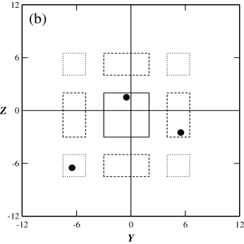
Figure 2: (a) Definition of signal and two sideband regions (arrowed brackets) in the $X$ distribution for the one-dimensional case. The width of each sideband region is half that of the signal region. (b) Definition of signal, sideband (dashed), and corner-band (dotted) regions in the $Y$ vs. $Z$ distribution for the two-dimensional case. The area of each sideband (corner-band) region is $\frac{1}{2}$ ($\frac{1}{4}$) that of the signal region.

3 Results

We have investigated the implication of including the Poisson uncertainty in the estimated background in the calculation of upper limits. In Tables 1-3, we give the 90% and 95% confidence level upper limits on the signal with and without including the Poisson uncertainty for several cases of small number of observed events and various backgrounds. The control regions have been chosen such that $\alpha=\frac{1}{2}$ and $\beta=\frac{1}{4}$. In the calculation of $\lambda_{0}$ with Eq. (1), the background is set to zero if $N_{cb}>2N_{sb}$. As expected, $\lambda$ is identical to $\lambda_{0}$ when the number of events in the signal region is zero, regardless of the number of estimated background events. However, $\lambda$ is smaller than $\lambda_{0}$ when the number of events in the signal region is non-zero and the estimated background is zero. This is not unexpected because Eqs. (6) and (7) allow for the estimated zero background to fluctuate up, in contrast to Eq. (1) in which the background is estimated to be zero with no uncertainty. This trend continues until the number of background events is comparable with the signal. When the number of background events is comparable or larger than the signal, the upper limit obtained is less stringent than that extracted without including the Poisson uncertainty in the estimated background. It is therefore important to incorporate the Poisson uncertainty into the upper limit; otherwise the upper limit obtained could be too stringent.

Table 1: Upper limits on the signal for a few observed events and various backgrounds in the one-dimensional case. The total width of the sideband regions is twice that of the signal region.

	90% C.L.		95% C.L.
($N_{ob}$,$\frac{N_{sb}}{2})$	$\lambda_{0}$	$\lambda$	$\lambda_{0}$	$\lambda$
(0,$\frac{N_{sb}}{2}$)	2.30	2.30	3.00	3.00
(1,0)	3.89	3.61	4.74	4.47
(1,$\frac{1}{2}$)	3.51	3.42	4.36	4.27
(1,1)	3.27	3.27	4.11	4.11
(1,$1\frac{1}{2}$)	3.11	3.16	3.94	3.99
(1,2)	3.00	3.07	3.82	3.90
(2,0)	5.32	4.94	6.30	5.92
(2,1)	4.44	4.36	5.41	5.33
(2,2)	3.88	3.96	4.82	4.91
(2,3)	3.52	3.68	4.44	4.61
(2,4)	3.29	3.47	4.18	4.39
(3,0)	6.68	6.26	7.75	7.34
(3,1)	5.71	5.53	6.78	6.61
(3,2)	4.93	4.96	5.98	6.03
(3,3)	4.36	4.53	5.40	5.58
(3,6)	3.48	3.74	4.42	4.73

Table 2: Upper limits on the signal for zero or one observed event and various backgrounds in the two-dimensional case. The total area of both the sideband and corner-band regions is four times that of the signal region.

	90% C.L.		95% C.L.
($N_{ob}$,$\frac{N_{sb}}{2}$,$\frac{N_{cb}}{4}$)	$\lambda_{0}$	$\lambda$	$\lambda_{0}$	$\lambda$
(0,$\frac{N_{sb}}{2}$,$\frac{N_{cb}}{4}$)	2.30	2.30	3.00	3.00
(1,0,$\frac{N_{cb}}{4}$)	3.89	3.61	4.74	4.47
(1,$\frac{1}{2}$,0)	3.51	3.48	4.36	4.33
(1,$\frac{1}{2}$,$\frac{1}{4}$)	3.67	3.51	4.53	4.36
(1,$\frac{1}{2}$,$\frac{1}{2}$)	3.89	3.53	4.74	4.38
(1,$\frac{1}{2}$,1)	3.89	3.55	4.74	4.40
(1,$\frac{1}{2}$,2)	3.89	3.57	4.74	4.43
(1,1,0)	3.27	3.35	4.11	4.20
(1,1,$\frac{1}{4}$)	3.38	3.40	4.22	4.25
(1,1,$\frac{1}{2}$)	3.51	3.44	4.36	4.29
(1,1,1)	3.89	3.49	4.74	4.33
(1,1,2)	3.89	3.53	4.74	4.38
(1,1,4)	3.89	3.57	4.74	4.42
(1,2,0)	3.00	3.14	3.82	3.98
(1,2,$\frac{1}{4}$)	3.05	3.21	3.88	4.05
(1,2,$\frac{1}{2}$)	3.11	3.26	3.94	4.11
(1,2,1)	3.27	3.35	4.11	4.19
(1,2,2)	3.89	3.44	4.74	4.29
(1,2,4)	3.89	3.51	4.74	4.36

Table 3: Upper limits on the signal for two observed events and various backgrounds in the two-dimensional case. The total area of both the sideband and corner-band regions is four times that of the signal region.

	90% C.L.		95% C.L.
($N_{ob}$,$\frac{N_{sb}}{2}$,$\frac{N_{cb}}{4}$)	$\lambda_{0}$	$\lambda$	$\lambda_{0}$	$\lambda$
(2,0,$\frac{N_{cb}}{4}$)	5.32	4.94	6.30	5.92
(2,1,0)	4.44	4.49	5.41	5.46
(2,1,$\frac{1}{2}$)	4.84	4.64	5.82	5.61
(2,1,1)	5.32	4.72	6.30	5.69
(2,1,2)	5.32	4.80	6.30	5.77
(2,1,4)	5.32	4.86	6.30	5.83
(2,2,0)	3.88	4.09	4.82	5.05
(2,2,$\frac{1}{2}$)	4.13	4.31	5.08	5.27
(2,2,1)	4.44	4.45	5.41	5.43
(2,2,2)	5.32	4.62	6.30	5.60
(2,2,4)	5.32	4.76	6.30	5.74
(2,2,6)	5.32	4.82	6.30	5.79
(2,4,0)	3.29	3.55	4.18	4.48
(2,4,$\frac{1}{2}$)	3.39	3.73	4.30	4.67
(2,4,1)	3.52	3.91	4.44	4.86
(2,4,2)	3.88	4.20	4.82	5.17
(2,4,4)	5.32	4.52	6.30	5.49
(2,4,6)	5.32	4.66	6.30	5.63

For a large number of observed events, we can use the common assumption that the signal $N_{0}$ in Eq. (2) is normally distributed (Gaussian) with the variance given by

$$\sigma^{2}=N_{ob}+\frac{1}{4}N_{sb}+\frac{1}{16}N_{cb},$$ (10)

where we set $\alpha=\frac{1}{2}$ and $\beta=\frac{1}{4}$. The upper limit on the number of signal events $\lambda_{G}$ is obtained by integrating from $N_{0}$ to $\lambda_{G}$ so that the integrated area is $\delta$ of the area integrated to $+\infty$. For an unphysical signal, $N_{0}<0$, the integration should be renormalized by setting $N_{0}=0$ to obtain a more conservative limit [2]. Tables 4-5 show a comparison of $\lambda_{G}$ and $\lambda$ for the case of $N_{ob}=N_{bg}$. Due to the longer tail of the Poisson distribution, $\lambda$ is larger than $\lambda_{G}$. The significance of the difference diminishes with larger $N_{ob}$. For example, in the one-dimensional case, it decreases from $\sim 10\%$ for $N_{ob}=10$ events to $\sim 5\%$ for $N_{ob}=50$ events. For an experiment with small systematic error, Eq. (6) or (7) should be used to compute the upper limit instead of using the Gaussian approximation.

Table 4: Upper limits on the signal for large number of observed events with large background in the one-dimensional case. The total width of the sideband regions is twice that of the signal region.

	90% C.L.			95% C.L.
($N_{ob}$,$\frac{N_{sb}}{2})$	$\lambda_{0}$	$\lambda$	$\lambda_{G}$	$\lambda_{0}$	$\lambda$	$\lambda_{G}$
(10,10)	6.63	7.24	6.35	8.08	8.78	7.59
(20,20)	8.75	9.82	8.98	10.60	11.83	10.74
(35,35)	11.11	12.69	11.88	13.41	15.24	14.20
(50,50)	13.00	15.00	14.20	15.66	17.98	16.97

Table 5: Upper limits on the signal for large number of observed events with large background in the two-dimensional case. The total area of both the sideband and corner-band regions is four times that of the signal region.

	90% C.L.			95% C.L.
($N_{ob}$,$\frac{N_{sb}}{2}$,$\frac{N_{cb}}{4}$)	$\lambda_{0}$	$\lambda$	$\lambda_{G}$	$\lambda_{0}$	$\lambda$	$\lambda_{G}$
(10,20,10)	6.63	8.61	7.78	8.08	10.31	9.30
(15,25,10)	7.78	9.86	8.98	9.45	11.82	10.74
(20,30,10)	8.75	10.93	10.04	10.60	13.10	12.00

For completeness, we also listed in Tables 6-8 the 90% and 95% confidence level upper limits on the signal for $\alpha=\beta=1$ with and without including the Poisson uncertainty in the estimated background for small number of observed events and various backgrounds.

Table 6: Upper limits on the signal for a few observed events and various backgrounds in the one-dimensional case. The total width of the sideband regions is the same as that of the signal region.

	90% C.L.		95% C.L.
($N_{ob}$,$N_{sb}$)	$\lambda_{0}$	$\lambda$	$\lambda_{0}$	$\lambda$
(0,$N_{sb}$)	2.30	2.30	3.00	3.00
(1,0)	3.89	3.51	4.74	4.36
(1,1)	3.27	3.27	4.11	4.11
(1,2)	3.00	3.11	3.82	3.94
(1,3)	2.84	3.00	3.64	3.82
(1,4)	2.74	2.91	3.53	3.72
(1,6)	2.62	2.78	3.39	3.58
(2,0)	5.32	4.75	6.30	5.72
(2,1)	4.44	4.32	5.41	5.29
(2,2)	3.88	4.01	4.82	4.97
(2,3)	3.52	3.77	4.44	4.72
(2,4)	3.29	3.59	4.18	4.52
(2,6)	3.01	3.33	3.86	4.23
(3,0)	6.68	5.99	7.75	7.08
(3,1)	5.71	5.43	6.78	6.52
(3,2)	4.93	4.99	5.98	6.06
(3,3)	4.36	4.63	5.40	5.69
(3,4)	3.97	4.35	4.97	5.39
(3,6)	3.48	3.93	4.42	4.94

Table 7: Upper limits on the signal for zero or one observed event and various backgrounds in the two-dimensional case. The total area of the sideband regions is twice that of the signal region while the total area of the corner-band regions is the same as that of the signal region.

	90% C.L.		95% C.L.
($N_{ob}$,$N_{sb}$,$N_{cb}$)	$\lambda_{0}$	$\lambda$	$\lambda_{0}$	$\lambda$
(0,$N_{sb}$,$N_{cb}$)	2.30	2.30	3.00	3.00
(1,0,$N_{cb}$)	3.89	3.51	4.74	4.36
(1,1,0)	3.27	3.38	4.11	4.22
(1,1,1)	3.89	3.42	4.74	4.27
(1,1,2)	3.89	3.44	4.74	4.29
(1,1,3)	3.89	3.45	4.74	4.30
(1,1,4)	3.89	3.46	4.74	4.31
(1,1,6)	3.89	3.47	4.74	4.32
(1,2,0)	3.00	3.27	3.82	4.11
(1,2,1)	3.27	3.34	4.11	4.18
(1,2,2)	3.89	3.38	4.74	4.22
(1,2,3)	3.89	3.40	4.74	4.25
(1,2,4)	3.89	3.42	4.74	4.27
(1,2,6)	3.89	3.44	4.74	4.29
(1,3,0)	2.84	3.18	3.64	4.02
(1,3,1)	2.99	3.27	3.82	4.11
(1,3,2)	3.27	3.32	4.11	4.17
(1,3,3)	3.89	3.36	4.74	4.20
(1,3,4)	3.89	3.38	4.74	4.22
(1,3,6)	3.89	3.41	4.74	4.25

Table 8: Upper limits on the signal for two observed events and various backgrounds in the two-dimensional case. The total area of the sideband regions is twice that of the signal region while the total area of the corner-band regions is the same as that of the signal region.

	90% C.L.		95% C.L.
($N_{ob}$,$N_{sb}$,$N_{cb}$)	$\lambda_{0}$	$\lambda$	$\lambda_{0}$	$\lambda$
(2,0,$N_{cb}$)	5.32	4.75	6.30	5.72
(2,1,0)	4.44	4.50	5.41	5.47
(2,1,1)	5.32	4.57	6.30	5.55
(2,1,2)	5.32	4.61	6.30	5.59
(2,1,3)	5.32	4.64	6.30	5.61
(2,1,4)	5.32	4.65	6.30	5.63
(2,1,6)	5.32	4.68	6.30	5.65
(2,2,0)	3.88	4.29	4.82	5.26
(2,2,1)	4.44	4.41	5.41	5.39
(2,2,2)	5.32	4.49	6.30	5.46
(2,2,3)	5.32	4.53	6.30	5.51
(2,2,4)	5.32	4.56	6.30	5.54
(2,2,6)	5.32	4.61	6.30	5.58
(2,3,0)	3.52	4.10	4.44	5.07
(2,3,1)	3.88	4.27	4.82	5.24
(2,3,2)	4.44	4.37	5.41	5.34
(2,3,3)	5.32	4.43	6.30	5.41
(2,3,4)	5.32	4.48	6.30	5.45
(2,3,6)	5.32	4.54	6.30	5.52
(2,4,0)	3.29	3.94	4.18	4.90
(2,4,1)	3.52	4.14	4.44	5.10
(2,4,2)	3.88	4.26	4.82	5.23
(2,4,3)	4.44	4.34	5.41	5.31
(2,4,4)	5.32	4.40	6.30	5.37
(2,4,6)	5.32	4.48	6.30	5.45

As noted in the previous section, Eq. (3) can also be used to calculate the upper limit on the signal for the case in which the background is estimated from a Monte Carlo simulation. The impact of including the Poisson uncertainty in the estimated background into the upper limit can be investigated by comparing the limit with that obtained without including the uncertainty. Table 9 lists the 90% confidence level upper limits obtained with and without including the Poisson uncertainty for several cases of small number of observed events and various backgrounds. As in the previous examples, $\lambda$ is smaller than $\lambda_{0}$ for small number of observed events with comparable or smaller background. However, $\lambda$ is larger than $\lambda_{0}$ for larger background. Not including the Poisson uncertainty leads to a too stringent limit in this case.

Table 9: 90% confidence level upper limits on the signal for small number of observed events and various backgrounds estimated from a Monte Carlo Simulation.

$\alpha^{-1}$	3		6		9
($N_{ob}$,$N_{sb}$)	$\lambda_{0}$	$\lambda$	$\lambda_{0}$	$\lambda$	$\lambda_{0}$	$\lambda$
(1,0)	3.89	3.67	3.89	3.76	3.89	3.80
(1,1)	3.61	3.51	3.74	3.65	3.79	3.71
(1,2)	3.42	3.38	3.61	3.55	3.70	3.64
(1,3)	3.27	3.27	3.51	3.47	3.61	3.57
(1,4)	3.16	3.18	3.42	3.40	3.54	3.51
(1,5)	3.07	3.11	3.34	3.33	3.48	3.45
(1,6)	3.00	3.05	3.27	3.27	3.42	3.40
(1,7)	2.93	3.00	3.21	3.22	3.37	3.36
(1,8)	2.88	2.95	3.16	3.17	3.32	3.31
(1,9)	2.84	2.91	3.11	3.13	3.27	3.27
(2,0)	5.32	5.04	5.32	5.17	5.32	5.22
(2,1)	5.00	4.79	5.16	5.02	5.21	5.11
(2,2)	4.70	4.57	5.00	4.88	5.10	5.01
(2,3)	4.44	4.38	4.84	4.75	5.00	4.92
(2,4)	4.22	4.21	4.70	4.63	4.89	4.82
(2,5)	4.04	4.07	4.57	4.51	4.79	4.73
(2,6)	3.88	3.94	4.44	4.41	4.70	4.65
(2,7)	3.74	3.82	4.33	4.31	4.61	4.57
(2,8)	3.62	3.72	4.22	4.22	4.52	4.49
(2,9)	3.52	3.63	4.13	4.13	4.44	4.42

4 Conclusion

We have presented a procedure for calculating an upper limit on the number of signal events which incorporates the Poisson uncertainty in the background estimated from control regions of one or two dimensions. For small number of observed events in the signal region, the limit obtained is more stringent than that extracted assuming no uncertainty in the estimated background. This trend continues until the number of background events is comparable with the signal. When the number of background events is comparable or larger than the signal, the upper limit obtained is less stringent than that extracted without including the Poisson uncertainty in the estimated background. It is therefore important to incorporate the Poisson uncertainty into the upper limit; otherwise the upper limit obtained could be too stringent.

5 Acknowledgment

This work was supported in part by the U.S. Department of Energy. K.K.G. thanks the OJI program of DOE for support.

References

[1]
G. Zech, Nucl. Instr. and Meth. A277 (1989) 608.
[2]
R.M. Barnett et al., Review of Particle Physics,
Phys. Rev. D54, (1996) 1.