[

Experiments on Critical Phenomena in a Noisy Exit Problem

Abstract

We consider noise-driven exit from a domain of attraction in a two-dimensional bistable system lacking detailed balance. Through analog and digital stochastic simulations, we find a theoretically predicted bifurcation of the most probable exit path as the parameters of the system are changed, and a corresponding nonanalyticity of the activation energy. We also investigate the extent to which the bifurcation is related to the local breaking of time-reversal invariance.

]

Noise-induced motion away from a locally stable state, in a system far from thermal equilibrium, arises in diverse scientific contexts, e.g., glasses [2], arrays of Josephson junctions [3], stochastically modeled computer networks [4], stochastic resonance [5], and stochastic ratchets [6]. Because these systems in general lack detailed balance, progress in understanding this phenomenon has been slower than in thermal equilibrium systems. In particular, there exist no simple or general relations from which the rate of noise-induced transitions between stable states can be obtained.

Recently, substantial progress on the nonequilibrium case has been achieved in the limit of weak noise, using path integral or equivalent Hamiltonian formulations [7, 8, 9, 10]. Fluctuational motion of the system can then be characterised by the pattern of optimal (i.e. most probable) fluctuational trajectories. An optimal trajectory is one along which a system moves, with overwhelming probability, when it fluctuates away from a stable state toward a specified remote state. These are rare events but, when they occur, they do so in an almost deterministic way: e.g. escape from a domain of attraction typically follows a unique trajectory. The properties of this most probable exit path (MPEP) determine the weak-noise behaviour of the mean first passage time (MFPT).

In recent years, it has been realized that in nonequilibrium systems, the pattern of optimal fluctuational trajectories may contain “focusing singularities” [10, 11]. Their effect on exit phenomena was considered by Maier and Stein [12, 13] who showed that, for a symmetric double well system (see below), the MPEP bifurcates when the model parameters are changed in such a way that a focusing singularity appears along it. That is, the MPEP ceases to be unique. This bifurcation breaks the symmetry of the model, and is accompanied by a nonanalyticity of the activation energy for inter-well transitions: it is analogous to a second-order phase transition in a condensed matter system [13]. This analogy throws new light on, e.g., exit bifurcation phenomena in systems driven by coloured noise [8].

Many of these theoretical ideas, although important, remain untested experimentally or numerically. In this Letter we use an analog experiment and numerical simulations to demonstrate the predicted bifurcation of the MPEP, and the corresponding nonanalytic behavior of the activation energy and related quantities. We investigate the nature of the broken symmetry in detail, and show how bifurcation is accompanied by a loss of time-reversal invariance along the MPEP.

We investigate the motion of an overdamped particle in the two-dimensional drift field first proposed in [9]: ${\bf u}(x,y)=(x-x^{3}-\alpha xy^{2},-y-x^{2}y)$, where $\alpha$ is a parameter. It has point attractors at $(\pm 1,0)$ and a saddle point at $(0,0)$. If the particle is subject to additive isotropic white noise ${\bf f}(t)=(f_{x},f_{y})$, its position $(x,y)$ will satisfy the coupled Langevin equations

$$\dot{x}=x-x^{3}-\alpha xy^{2}+f_{x}(t),$$ (1)

$$\dot{y}=-y-x^{2}y+f_{y}(t),$$ (2)

$$\langle f_{i}(t)\rangle=0,\quad\langle f_{i}(s)f_{j}(t)\rangle=D\delta_{ij}\delta(s-t).$$ (3)

Since ${\bf u}$ is not a gradient field (unless $\alpha=1$), the dynamics will not satisfy detailed balance. The Fokker–Planck equation for the particle’s probability density $\rho=\rho(x,y,t)$ will be

$$\dot{\rho}=(D/2)\nabla^{2}\rho-{\bf\nabla\cdot}(\rho{\bf u}).$$ (4)

In the weak-noise limit, escape of the particle from the domain of attraction of either fixed point $(x_{s},0)=(\pm 1,0)$ is governed by the the slowest-decaying nonstationary eigenmode of the Fokker–Planck operator [14], whose eigenvalue $\lambda_{1}$ becomes exponentially small as ${D\to 0}$. In this limit the MFPT $\langle t_{\rm exit}\rangle$ is well approximated by $\lambda_{1}^{-1}$. The slowest-decaying eigenmode is called the quasistationary probability density; we denote it by $\rho_{1}$. It may be approximated in a WKB-like fashion [9, 12, 13], i.e.,

$$\rho_{1}(x,y)\sim K(x,y)\exp\left(-W(x,y)/D\right),\qquad D\to 0.$$ (5)

Here $W(x,y)$ may be viewed as a classical action at zero energy, since it turns out to satisfy an eikonal (Hamilton–Jacobi) equation of the form $H({\bf x},{\bf\nabla}W)=0$, where $H({\bf x},{\bf p})=\frac{1}{2}{\bf p}^{2}+{\bf u}({\bf x})\cdot{\bf p}$ is a so-called Wentzel–Freidlin Hamiltonian [15]. The optimal fluctuational trajectories are projections onto coordinate space of the zero-energy classical trajectories determined by this Hamiltonian. These lie on the three-dimensional energy surface specified by ${H=0}$, embedded in the four-dimensional phase space with coordinates $(x,y,p_{x},p_{y})$. In general, the computation of $W(x,y)$ requires a minimisation over the set of zero-energy trajectories starting at $(x_{s},0)$ and terminating at $(x,y)$. Moreover the MPEP, for the domain of attraction of $(x_{s},0)$, is the zero-energy trajectory of least action which extends from $(x_{s},0)$ to the saddle $(0,0)$. The MPEP action $\delta W\equiv W(0,0)-W(x_{s},0)$ governs the weak-noise behavior of the MFPT. To leading order it is of the activation type, i.e.,

$$\langle t_{\rm exit}\rangle\sim{\rm const}\times e^{\delta W/D},\qquad D\to 0.$$ (6)

So $\delta W$ is interpreted as an activation energy. The prefactor ‘const’ is determined by the function $K(x,y)$ of (5).

When $\alpha=1$, the dynamics of the particle satisfy detailed balance, and the pattern of optimal trajectories emanating from $(x_{s},0)$ contains no singularities. It was found earlier [12, 13] that, as $\alpha$ is increased, the first focusing singularity on the MPEP (initially lying along the $x$-axis) appears when $\alpha=\alpha_{c}\equiv 4$. It signals the appearance of a transverse ‘soft mode,’ or instability, which causes the MPEP to bifurcate. Its physical origin is clear: as $\alpha$ is increased, the drift toward $(x_{s},0)$ ‘softens’ away from the $x$-axis, which eventually causes the on-axis MPEP to split. The two new MPEP’s move off-axis, causing the activation energy (previously constant) to start decreasing. So the activation energy as a function of $\alpha$ is nonanalytic at $\alpha=\alpha_{c}$. If $\alpha$ is increased substantially beyond $\alpha_{c}$, further bifurcations of the on-axis zero-energy classical trajectory occur when $\alpha$ equals $\alpha_{c}^{(j)}\equiv(j+1)^{2}$, where $j$ is the number of the bifurcation. But the oscillatory trajectories arising from such bifurcations are believed to be unphysical, since the on-axis trajectory is no longer the MPEP. (Cf. [10].)

To test these theoretical predictions, and to seek further insight into the nature of the broken symmetry, we have built an analog electronic model of the system (2) using standard techniques [16]. We drive it with zero-mean quasi-white Gaussian noise from a noise-generator, digitize the response $x(t),y(t)$, and analyse it with a digital data processor. Transition probabilities are measured by a standard level-crossing technique. Experimental investigations of the optimal fluctuational trajectories are based on measurements of the prehistory probability distribution [17, 18]. This method was recently extended to include analysis of relaxational trajectories and thus to investigate directly the presence or absence of time-reversal symmetry and detailed balance [19].

We have also carried out a complementary digital simulation of (2) using the algorithm of [20], with particular attention paid to the design of the noise-generator on account of the long simulation times. Transition probabilities were measured using a well-to-well method, and the analysis of the data to extract the optimal fluctuational and relaxational trajectories was based on a method similar to that used in the analog experiments.

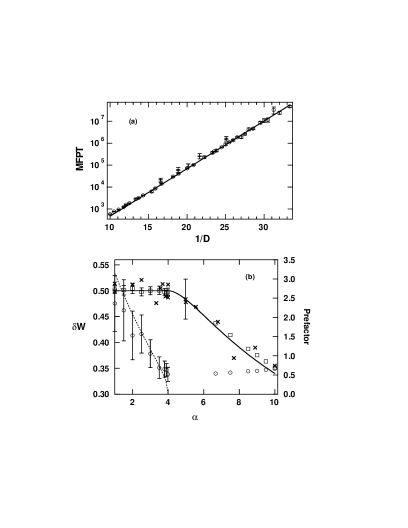
FIG. 1.: (a) The mean first passage time as a function of inverse noise intensity $1/D$ for $\alpha=1$, from analog experiment (bars), numerical simulation (circles) and calculation (solid line). (b) The inter-well activation barrier $\delta W$, as a function of $\alpha$, from analog experiment (crosses), numerical simulation (squares) and theory [12, 13] (full line). The dashed curve and circle data represent the MFPT prefactor from calculation and numerical simulation respectively.

Some activation energy results are shown in Fig. 1. Part (a) plots the MFPT $\langle t_{\rm exit}\rangle$ as a function of inverse noise intensity $1/D$ for the special case $\alpha=1$. In this case the drift field is the gradient of the potential $U(x,y)=\bigl{(}y^{2}(1+x^{2})-x^{2}+x^{4}/2\bigr{)}/2$, and $W$ can be obtained exactly ($W=2U$). The analog and digital results are in good agreement, and demonstrate that the noise dependence of the MFPT is indeed of the activation type predicted by the theory. Activation energies determined from the slopes of a series of plots like those in Fig. 1(a), yielded the results shown in Fig. 1(b), where they are compared with theoretical values of $\delta W$ determined from the true (least action) MPEP or MPEP’s [12, 13]. At the predicted critical value $\alpha_{c}=4$, marked changes in both the activation energy and MFPT prefactor (which $\rightarrow 0$) are evident: theory predicts that the activation energy bifurcates here into two values, corresponding to paths on and off the $x$-axis, of which only the latter (lower action) path is expected to be physically meaningful. The dependence of the activation energy on $\alpha$ near the second critical value $\alpha_{c}^{(2)}\equiv 9$ is smooth, in agreement with the prediction that higher bifurcations correspond to folding of a nonphysical sheet of the ‘action surface’ $W=W(x,y)$, and are not observable [10, 13].

Interestingly, the transition shown in Fig. 1(b) resembles the bifurcation of the activation energy in an overdamped oscillator driven by coloured noise [8]. This suggests that the WKB analysis [12, 13] of (2) may provide physical and topological insight into the corresponding transition phenomena in systems driven by quasi-monochromatic noise.

FIG. 2.: Measured positions of the ridges (first moments) for $\alpha=6.67$ of (a) the fluctuational part (filled circles) and (b) the relaxational part (pluses) of the escape trajectories. Nearby theoretical trajectories are shown by lines. The insert shows the exit location distribution along the $y$-axis.

To verify experimentally the expected relationship between the bifurcation of the MPEP and the bifurcation of the activation energy, we have measured two-dimensional prehistory probability distributions [17] of fluctuational trajectories bringing the system into the vicinity of the separatrix between the two wells (the $y$-axis). In the limit of low noise intensity, the maxima of the corresponding distributions trace out optimal trajectories [18, 19]. The positions of these maxima are compared to the calculated MPEP’s for $\alpha=6.67$ in Fig. 2(a). It is clear that the typical fluctuational path corresponding to escape from the domain of attraction of $(x_{s},0)$ follows very closely one of the predicted MPEP’s.

To seek further experimental insight into the character of the broken symmetry for the MPEP, we have also followed the dynamics of the relaxational part of the escape paths, after they have crossed the $y$-axis separatrix. The prehistory and relaxational probability distributions provide a complete history of the time evolution of large fluctuations to and from a given remote state. One can thus investigate experimentally detailed balance and time-symmetry (or the lack of them) [19]. The positions of the maxima of the measured relaxational distributions are compared with the corresponding theoretical trajectories in Fig. 2(b). A detailed analysis of the distributions will be given elsewhere. It can be seen from the figure that for $\alpha>\alpha_{c}$ the MPEP breaks time-reversal symmetry, i.e., the average growth and average decay of fluctuations [21] traced out by the ridges of the corresponding distributions take place along trajectories that are asymmetric in time. That is, for $\alpha>\alpha_{c}$ the MPEP is not a time-reversed relaxational trajectory.

The inset in Fig. 2(b) shows the distribution of points where the escape trajectories hit the $y$-axis separatrix (i.e., the exit location distribution). Its shape is nearly Gaussian, as expected from the saddle point approximation of [13]. The maximum is situated near the saddle point clearly demonstrating that, in the limit of weak noise, exit occurs via the saddle point.

The relationship between time-reversal symmetry-breaking for the MPEP when ${\alpha>\alpha_{c}}$, and symmetry-breaking generally for the system (2), is quite subtle. The system loses detailed balance and time reversal symmetry as soon as $\alpha>1$  and the drift field $\bf u$ becomes nongradient. It is on account of a special symmetry of the system (reflection symmetry through the $x$-axis) that the MPEP can remain unchanged in this nongradient drift field up to the value $\alpha_{c}=4$. Thus, for $1<\alpha<4$ the dynamics of the most probable fluctuational trajectories is a mirror-image of the relaxational dynamics only along the $x$-axis; everywhere else in the domain of attraction of $(x_{s},0)$ the outward optimal trajectories are not antiparallel to the inward relaxational trajectories, and the resulting closed loops enclose nonzero area [12, 15].

FIG. 3.: Demonstration of local properties of detailed balance and time-reversal symmetry of (2) for $\alpha=3.5$. (a) Measured positions of the ridges of the fluctuational (filled circles) and relaxational (pluses) parts of the trajectories from $(1,0)$ to $(0.3,0.3)$, compared with theoretical predictions [12, 13] (curves). (b) The same for trajectories extending to the on-axis remote state $(0.1,0)$.

This prediction has been tested experimentally by tracing out optimal paths to/from specified remote states both on and off the $x$-axis, for $1<\alpha<\alpha_{c}$. Some results are shown in Fig. 3 for $\alpha=3.5$. It is evident that the ridges of the fluctuational (filled circles) and relaxational (pluses) distributions follow closely the theoretical curves. For an off-axis remote state (Fig. 3(a)), they form closed loops of nonzero area, thus demonstrating the expected rotational flow of the probability current in a nonequilibrium system [21]. The corresponding ridges for an on-axis remote state (Fig. 3(b)) are antiparallel, indicating that symmetry is preserved along the $x$-axis.

Our results verify the predicted bifurcation of the MPEP in (2) at $\alpha=\alpha_{c}\equiv 4$, with a corresponding nonanalyticity of the activation energy. We have demonstrated that, in the limit $D\to 0$, detailed balance and time-reversal symmetry can be considered as local properties along the MPEP of the system in the sense discussed above, and that the bifurcation phenomenon can be related to local time-reversal symmetry-breaking along the MPEP: results that may bear on two-dimensional stochastic ratchets [22] where symmetry plays an important role. Having thus demonstrated (see also [18]) the reality of phenomena inferred from $D\to 0$ optimal paths, we anticipate that other important $D\to 0$ theoretical predictions, e.g. “cycling” of the exit location distribution [23], will also be physically realisable.

The research was supported by the Engineering and Physical Sciences Research Council (UK), the Royal Society of London, the Russian Foundation for Basic Research, the National Science Foundation (US), and the Department of Energy (US).

REFERENCES

- [1] Permanent address: Institute of Metrological Service, Ozernaya 46, Moscow 119361, Russia.
- [2] D. L. Stein, R. G. Palmer, J. L. van Hemmen, and C. R. Doering, Phys. Lett. A 136, 353 (1989).
- [3] R. L. Kautz, Rep. Progr. Phys. 59, 935 (1996).
- [4] R. S. Maier, in Proc. 33rd Annual Allerton Conference on Communication, Control, and Computing (Monticello, Illinois, Oct. 1995), 766.
- [5] See special issue of Nuovo Cim. D 17, nos. 7–8 (1995); A. R. Bulsara and L. Gammaitoni, Phys. Today 49, no. 3, 39 (1996).
- [6] M. Magnasco, Phys. Rev. Lett. 71, 1477 (1993).
- [7] A. J. Bray and A. J. McKane, Phys. Rev. Lett. 62, 493 (1989).
- [8] S. J. B. Einchcomb and A. J. McKane, Phys. Rev. E 51, 2974 (1995).
- [9] R. S. Maier and D. L. Stein, Phys. Rev. E 48, 931 (1993).
- [10] M. I. Dykman, M. M. Millonas, and V. N. Smelyanskiy, Phys. Lett. A 195, 53 (1994), cond-mat/9410056; V. N. Smelyanskiy, M. I. Dykman, and R. S. Maier, Phys. Rev. E 55, 2369 (1997).
- [11] H. R. Jauslin, Physica 144A, 179 (1987); M. V. Day, Stochastics 20, 121 (1987).
- [12] R. S. Maier and D. L. Stein, Phys. Rev. Lett. 71, 1783 (1993).
- [13] R. S. Maier and D. L. Stein, J. Stat. Phys. 83, 291 (1996), cond-mat/9506097.
- [14] B. Carmeli, V. Mujica, and A. Nitzan, Berichte der Bunsen-Gesellschaft 95, 319 (1991).
- [15] M. I. Freidlin and A. D. Wentzell, Random Perturbations of Dynamical Systems (Springer-Verlag, New York/Berlin, 1984).
- [16] L. Fronzoni, in Noise in Nonlinear Dynamical Systems, edited by F. Moss and P. V. E. McClintock (Cambridge University Press, Cambridge, England, 1989), vol. 3, 222; P. V. E. McClintock and F. Moss, op. cit., 243.
- [17] M. I. Dykman, P. V. E. McClintock, V. N. Smelyanskiy, N. D. Stein, and N. G. Stocks, Phys. Rev. Lett. 68, 2718 (1992).
- [18] M. I. Dykman, D. G. Luchinsky, P. V. E. McClintock, and V. N. Smelyanskiy, Phys. Rev. Lett. 77, 5229 (1996).
- [19] D. G. Luchinsky, “On the nature of large fluctuations in equilibrium systems: Observation of an optimal force”; D. G. Luchinsky and P. V. E. McClintock, “Irreversibility of classical fluctuations.” To be published.
- [20] R. Mannella, “Numerical integration of stochastic differential equations,” in Proc. Euroconference on Supercomputation in Nonlinear and Disordered Systems (World Scientific, Singapore, in press).
- [21] L. Onsager, Phys. Rev. 37, 405 (1931).
- [22] G. W. Slater, H.-L. Guo, and G. I. Nixon, Phys. Rev. Lett. 78, 1170 (1997).
- [23] M. V. Day, Stochastics 48, 227 (1994); J. Dynamics and Differential Equations 8, 573 (1996); R. S. Maier and D. L. Stein, Phys. Rev. Lett. 77, 4860 (1996), cond-mat/9609075.