The Time-Dependent Local Density Approximation for Collective Excitations of Atomic Clusters

Abstract

We discuss the calculation of collective excitations in atomic clusters using the time-dependent local density approximation. In principle there are many formulations of the TDLDA, but we have found that a particularly efficient method for large clusters is to use a coordinate space mesh and the algorithms for the operators and the evolution equations that had been developed for the nuclear time-dependent Hartree-Fock theory. The TDLDA works remarkably well to describe the strong excitations in alkali metal clusters and in carbon clusters. We show as an example the benzene molecule, which has two strong features in its spectrum. The systematics of the linear carbon chains is well reproduced, and may be understood in rather simple terms.

I Introduction

The time-dependent local density approximation (TDLDA) is a powerful tool to calculate the quantum mechanical motion of electrons in condensed matter systems. In my talk I want to describe to you the numerical techniques we use ya96 , which were borrowed from nuclear physicsfl78 . I then want to show you a survey of some of the results, concluding with new work on the behavior of electrons in elongated chains. The time-independent LDA is known as Density Functional Theory and is well-established in condensed matter physics jo89 as a predictive ab initio theory that is practical for structures beyond the range of quantum chemistry methods [4-7]. The equations of the LDA are easy to write down. The energy function is given by the expression

$$E=\int d^{3}r\Biggl{[}\sum_{i}{|\nabla\phi_{i}|^{2}\over 2m}++\sum_{I}V_{ion}(r-r_{I})\rho(r)+$$ (1)

$$+{1\over 2}\int d^{3}r^{\prime}{e^{2}\over|r-r^{\prime}|}\rho(r)\rho(r^{\prime})+v_{ex}\bigl{(}\rho(r)\bigr{)}\Biggr{]}$$

where the $\phi_{i}$ are the single-particle wave functions and $\rho(r)=\sum_{i}|\phi_{i}(r)|^{2}$ is the density. The potentials included in the energy function are $V_{ion}$, the ionic potential, $e^{2}/|r-r^{\prime}|$, the direct Coulomb interaction between electrons, and $v_{ex}(\rho)$, the local-density approximation to the exchange-correlation energy. The static LDA theory is obtained by minimizing this energy function, requiring only that the $\phi_{i}$ be orthonormal. That gives the Kohn-Sham equations for the wave functions $\phi_{i}$. The TDLDA equations are very similar, with the “energy” (actually the Lagrange multiplier) in the Kohn-Sham equation replaced by the time derivative $i\hbar\partial_{t}$,

$$i\hbar\partial_{t}\phi_{i}(\vec{r},t)=H\phi_{i}(\vec{r},t).$$ (2)

with

$$H=-\frac{\hbar^{2}}{2m}\nabla^{2}+\sum_{I}V_{ion}(\vec{r}-\vec{R}_{I})+e^{2}\int d\vec{r}^{\prime}\frac{\rho(\vec{r}^{\prime},t)}{|\vec{r}-\vec{r}^{\prime}|}+{dv_{xc}\over d\rho}\Big{|}_{r,t}.$$

This is almost all I want to say in general. One always uses pseudopotentials for the ionstr91 ; kl82 , to eliminate the core electrons with their large energy scales. The LDA has well-known difficulties in describing the electronic excitations of systems, attributable to the simplified treatment of exchange. However, the collective motion is rather insensitive to the nonlocality of the exchange, and the TDLDA is much more reliable than one would expect from looking at energy gaps.

II Numerical

For most applications it is sufficient to consider small deviations from the static solution, and then there are a number of approaches to solve the small-amplitude TDLDA equations. Nuclear physicists are most familiar with the configuration representation, which I’ll just mention briefly. Here one represents the time-dependent wave function in the basis of the static solutions,

$$\phi_{i}(t)=\phi_{i}(0)+\sum_{j}a_{ij}(t)\phi_{j}(0).$$ (3)

The equation of motion is Fourier transformed to frequency, and the matrix equations satisfied by the particle-hole amplitudes $\tilde{a}_{ij}(\omega)$ are the RPA equations of motion. This method becomes inefficient for large systems, because the the dimensionality of the matrix grows as the product of the number of particle and hole orbitals. In the more efficient methods, the dimensionality increases linearly with the number of particles. One method that is very popular is to calculate the density-density response function. This is the density change induced at a point $r$ by a density perturbation at a point $r^{\prime}$. Because of the local density approximation, one can calculate the full response from the response of non-interacting electrons. The number of mesh points to represent the response increases as the volume of the system, and thus only linearly with the number of particles, making it more efficient for large systems. The method has been used extensively for systems with spherical symmetryek84 ; be75 ; recently it has been applied also to clusters in three dimensionsru96 .

We use another method whose dimensionality also scales linearly with the system size. This is the straightforward solution of the time-dependent equations of motion. The number of variables is the number of points at which wave function amplitudes are represented. This can be of the order of 50,000 for some of the examples we consider, so some care must be taken to use efficient numerical algorithms. We have simply adopted the technique of ref. fl78 who investigated the TDHF theory of nuclear dynamics.

We use a uniform mesh in coordinate space to represent the wave function. The shape of the gridded volume can be spherical, cylindrical, or rectangular, depending on the cluster under consideration. If the equations were linear in $\phi$, they could efficiently integrated by using the Taylor series expansion of the evolution operator, $\phi(t)=\exp(-iHt)\phi=1+tH\phi+t^{2}H^{2}\phi/2+...$ In practice we can ignore the change of H dependence of $H$ on $\phi$ for some small time interval $\tau$, and use the Taylor series integrator over that interval. We typically use fourth order:

$$e^{-iH\tau}\phi=\sum_{n=0}^{4}{(i\tau)^{n}\over n!}H^{n}\phi$$ (4)

Considerable care must be given to defining the $H$ to propagate in the above equation. An important consideration is that the algorithm conserve energy to a very high accuracy. This can be assured with an implicit definition of $H$ in terms of the densities $\rho(t)$ and $\rho(t+\tau)$ at the beginning and end of the interval $\tau$. The definition is

$$H\phi(r)=\Big{[}{-\nabla^{2}\over 2m}+{v\big{(}\rho(r,t+\tau)\bigr{)}-v\big{(}\rho(r,t)\bigr{)}\over\rho(r,t+\tau)-\rho(r,t)}\Bigr{]}\phi(r).$$ (5)

In practice we do not calculate this exactly but rather estimate the Hamiltonian at $t+\tau/2$ using a predictor-corrector method. In our algorithm, first the potential is extrapolated forward by half a time step with a 3-point difference formula to get a trial potential $V_{trial}(t+\tau/2)$. The time integration is then performed using $V_{trial}$ to get a trial density $\rho_{trial}(t+\tau)$, and the density at time $t+\tau/2$ is estimated as $\rho(t+\tau/2)=(\rho(t)+\rho_{trial})/2$. The potential obtained with this density is used to once more integrate the wave function from $t$ to $t+\tau$.

To generate the response of the system, we perturb the ground state wave function and measure the response as a function of time. The initial wave functions are taken as $\phi_{i}(\vec{r},0)={\rm e}^{ikz}\phi_{i}^{o}(\vec{r})$ in which $\phi_{i}^{o}$ represent the static Kohn-Sham solutions. We are interested in the optical response, requiring the perturbing parameter $k$ to is small. This ensures also that the response will be in the linear regime. The real time evolution of the dipole moment is obtained as $z(t)=\sum_{i}<\phi_{i}(t)|z|\phi_{i}(t)>,$ and its Fourier transform in time gives the dipole strength function.

Summarizing, our algorithm to integrate the TDLDA equations has as numerical parameters the spatial mesh size, $\Delta x$, the number of mesh points $M$, the time step $\tau$, and the total length of time integration $T$. The actual values for the different systems will be given below.

III Physics

Our interest is in the electronic excitations, and we will leave aside completely the problem of determining the ionic geometries of the clusters. In classical electromagnetic theory, the dipole strength in spherical metal clusters is concentrated in the Mie resonance. The resonance may be sharp or not depending on the cluster, and it may be present also in clusters of different shapes.

III.1 Alkali metals

The simple, sharp Mie resonance behavior is reproduced by jellium model of alkali metal clustersek84 , which however neglect the perturbing effects of the ionic cores. It is therefore interesting to see to what extent the ionic cores affect the physics. I will first consider a system where the jellium approximation is remarkably good. This is the for clusters of sodium atoms. An example of a calculation is the sodium cluster Na₁₄₇. This was chosen because 147 atoms can be placed in a icosahedral structure, which is as close a one can get to spherical structure with discrete atoms. The numerical parameters of the calculation are: $\Delta x=0.8$ Å, $\tau/\hbar=0.01$ eV^-1, $M=28000$ and $N_{t}=5000$. Because the valence electron is in an $s$-wave, and the short-distance part of the wave function has been smoothed away by the pseudopotential, a rather coarse $\Delta x$ is sufficient. The total time integration is $\tau N_{t}/\hbar=50$ eV^-1 which in principle allows structures on the scale of 0.02 eV to be resolved. Fig. 1 shows the response, compared with the spherical jellium model. Both descriptions show a sharp peak at just over 3 eV excitation, and some background extending in both directions. The two theories are quite close. This shows that the pseudopotential in sodium has little effect. Experimentally, sodium clusters show a fairly sharp resonance, but the energy is lower by about 15%.

Figure 1: Dipole response of a sodium cluster, Na${}_{147}^{+}$, comparing the spherical jellium model with the full pseudopotential TDLDA calculation.

Figure 2: Dipole response of lithium clusters, comparing the jellium model, the full TDLDA calculation, and experiment [13].

The next case, lithium, shows a more dramatic difference between the jellium model and the full pseudopotential TDLDA. Fig. 2 shows the response of Li${}_{147}^{+}$, comparing the full pseudopotential LDA with the jellium model. The Mie resonance has been shifted down by the pseudopotential interactions and broadened. The reason for the difference compared to sodium is not hard to findya95 . The scattering effect of the pseudopotential is much larger in the case of Li, and the scattering gives the electrons an effective mass larger than one. In the jellium model the ion behaves as a uniform positive charge density filling space within the lattice. The scattering effect of the pseudopotential may be seen by examining the scattering from the difference between the pseudopotential and a uniform positive charge. Thus, we are led to examine the scattering from the difference potential,

$$\Delta V=V_{i}(r)+{e^{2}\over r_{0}}\Big{(}{3\over 2}-{1\over 2}({r\over r_{0}})^{2}\Big{)}~{}~{}~{}~{}r<r_{s}$$

$$=V_{i}(r)+{e^{2}\over r}~{}~{}~{}~{}r>r_{s}$$

When we do this we find that both the $s$- and $p$-wave scattering phase shifts for sodium are small, showing that effects of the pseudopotential are weak. On the other hand, in the case of Li, the $s$-potential is repulsive but the $p$-wave potential is attractive. This implies that there will be a large backward angle scattering, making the single-particle wave functions rather different than the jellium wave functions. We believe this aspect is responsible for the broadening of the Mie resonance in Li. Another consequence of the two potentials is that the effective forward scattering potential will be momentum-dependent, becoming more attractive as the momentum increases and the amount of $p$-wave increases. This lowers the Mie resonance frequency.

III.2 Carbon structures

Carbon is more difficult because the $p$-valence electrons are rather tightly bound and require a finer mesh. In practice, a mesh size of $\Delta x=0.3$ Å is adequate to calculate the electronic response of carbon structures, given their geometry. As a first test, we examine the response of the benzene molecule, which has been well-studied up to 30 eV with synchrotron photon sourcesko72 ; hi91 . For the calculation, we used a pseudopotential for the hydrogen atoms as well as the carbon atoms, and used the actual geometry of the molecule. The grid of mesh mesh points was limited to points in a sphere of radius 7 Å. This requires about 50,000 mesh points. Finally, because of the tighter binding of the $p$-waves, a time step a factor of 10 smaller than that for the alkali metals was required, $\tau=0.001$ eV^-1. The resulting response is plotted in Fig. 3, showing the Fourier transform of the real-time response computed over a time interval of 30 $\hbar$/eV. This is compared to the strength function measured in ref. ko72 , which an adjusted normalization (which was arbitrary in ref. ko72 . The main features of the response are a sharp peak at 6.9 eV, and a broad bump centered just below 20 eV. The sharp peak is very well reproduced by theory. It is associated with a collective resonance of the $\pi$ electrons. The calculated strength of the resonance $f$ is =1.1 in the usual sum rule units (i.e. the effective number of electrons). The experimental strength can be extracted from the data of ref. hi91 , but the peak shape has wings that are not simple Lorentzian tails. Including the right-hand wing up to 8.3 eV, but not the left-hand shoulder, the measured strength is $f=0.9$, which we consider rather good agreement. The large broad bump is associated with the $\sigma$ electrons. We reproduce its gross structure. But note that the theoretical distribution has much finer structure than is observed experimentally.

Figure 3: In-plane dipole response of benzene molecule, comparing TDLDA with experiment [15].

Our next example is C₆₀. Our TDLDA calculation is shown in Fig. 4, together with another TDLDA calculation using the matrix RPA methodya93 . In our calculation, the $\pi$ electron excitation appears as a single peak at 7 eV, carrying a strength of $f=9$. Experimentally, the $\pi$ electron transitions are split into several peaks, with a total strength up to 7 eV of $f=6$. There are no absolute measurements of the strength above 7 eV, but photoionization measurements exist he92 that show a broad $\sigma$ resonance, as in benzene. The (unnormalized) data is shown in the figure with diamond symbols. The polarizability of C₆₀ has some interest, because the simplified tight-binding model gave a number much smaller than experiment, $\alpha\approx 45$ ų compared to the experimental value $\alpha\approx 85$ ų. The polarizability may be extracted from the dipole strength function by the integral

$$\alpha={e^{2}\over m}\int{df\over dE}{dE\over E^{2}}.$$ (6)

The result is 80 ų, in satisfactory agreement with experiment.

Figure 4: Response of C₆₀ in TDLDA. The dashed curve is another TDLDA calculation, using the particle-hole matrix formulation [18].

III.3 Carbon chains

The important role of geometry in the dipole response is beautifully illustrated by the collective $\pi$ transition in carbon chains and rings. For these calculationsya97 , we guessed at the geometry, fixing the nearest neighbor distance at 1.28 Å for all cases. This is the average LDA equilibrium distance for large rings or chains. The atoms are in a line on the chains and form a circle on the rings. As in the other examples, there is a strong collective $\pi$ transition along the axis of the chain or in the plane of the ring. The energies of the excitations are plotted in Fig. 5 as a function of the number of atoms. There is experimental data showing the existence of excitations at the predicted energies for chains fo96 . Unfortunately, the strengths of the transitions were not measured, so it is not known whether the observed transitions really correspond to the calculated collective excitations. The stable form of carbon for cluster numbers greater than ten or so is believed to be the ring configuration, but no data is available on this form.

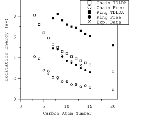
Figure 5: Excitation energies of TDLDA collective states and single-particle excitations in carbon chain and rings. The crosses mark experimentally observed excitations [20-22].

Notice that the excitation energies have a strong but smooth dependence on the chain length. The variation is entirely explicable in terms of simple physics, not requiring at all the detailed TDLDA calculations. This is the theme of the next section of my talk.

IV Collective energetics in atomic chains

The behavior of electromagnetic resonances on infinitely long wires is known from classical electromagnetic theory. The dispersion formula for the one-dimensional plasmon on a long wire reduces to the following expression in the long-wave length, thin wire limitgo90 ; li91 .

$$\omega^{2}={4\pi n_{e}e^{2}\over m}q^{2}\log{1\over qa}$$ (7)

where $q$ is the reduced wave number of the plasmon, $n_{e}$ is the density of electrons per unit length, and $a$ is the radius of the wire. For a finite wire, the lowest mode would have a $q$ varying inversely with the length of the wire $L$. Thus the lowest mode would behave as

$$\omega\sim C{\sqrt{\log(L/a)}\over L}$$ (8)

This behavior can be extracted from a more quantum approach is the polarizability estimate of the collective frequencyde93 ,

$$\omega^{2}={\hbar^{2}e^{2}N_{e}\over m\alpha}$$ (9)

where $N_{e}$ is the number of active electrons and $\alpha$ is the polarizability. This formula is derived from the ratio of sum rules, and $N_{e}$ may be identified with the oscillator strength $f$ associated with the transition. For the linear carbon chains, the transition is associated with $\pi$ electrons and and the number of them in the chain $C_{n}$ ($n$ odd) is

$$N_{e}=2n-2.$$

The TDLDA calculations confirm that this is satisfied at the level of 20% accuracy. The polarizability is harder to estimate. In ref. ya97 we model the polarizability assuming that the chain acts as a perfectly conducting wire, of some fixed transverse dimension $a$ and a long length $L$. Then one can show that for large $L$ the polarizability is given by

$$\alpha\approx{L^{3}\over 24\log(L)}$$

The dependence on the number of atoms in the chain follows form $L\sim n$. Then inserting the above in eq. (9), we find the large-$n$ behavior

$$\omega\sim{\sqrt{\log n}\over n}.$$ (10)

This is plotted in Fig. 6 as the solid line, fitted to the TDLDA result at $n=14$. We see that the general trend is reproduced, but the asymptotic behavior is only realized in long chains.

Figure 6: Comparison of analytic formulas with the energy systematics of carbon chains. Solid line, eq. (10); dashed line, eq. (11).

Another classical view is to compare with the polarizability of a conducting ellipsoid, which can be calculated analyticallybo83 . The formula is

$$\omega^{2}={1-e^{2}\over e^{2}}\Big{(}-1+{1\over 2e}\log{1+e\over 1-e}\Big{)}\omega_{0}^{2}$$ (11)

where $e$ is related to the ratio of short to long axes, $R_{\perp}/R_{\parallel}$,

$$e^{2}=1-\Big{(}{R_{\perp}\over R_{\parallel}}\Big{)}^{2}.$$ (12)

This has been applied to the longitudinal mode in fullerines br96 . Its asymptotic behavior is given by eq. (10) above. Remarkably, this formula gives an excellent fit, treating the two parameters as adjustable. This is shown as the dashed curve in Fig. 5.

We finally discuss the relative frequencies of the modes in chains and rings. One expects that for C_n in the form of rings, the number of $\pi$ electrons is $2n$, roughly the same as chains. However, the polarizability will be quite a bit smaller because of the more compact geometry. The ratio of polarizabilities is about a factor of two, giving a prediction of a 40% higher collective resonance. In fact the TDLDA calculations shows that the sum rule $f$ is also higher for ring configurations, and the actual resonance is at about twice the energy of the chain. This may be seen in Fig. 5.

V What next?

We have discussed carbon, but from a computational point of view the next group IV element, silicon, would be very similar. The next challenge for numerical TDLDA would be the group IB metals, the so-called coinage metals. These have a single valence electron in an $s$ shell, like the alkali metals, but there is a nearby closed $d$ shell that cannot be neglected in the response. Beyond that, there are all $d$-shell metals which exhibit broad responses, hardly showing any trace of the Mie resonance. But this remains for the for the future.

VI Acknowledgment

We thank R.A. Broglia for calling our attention to eq. (11). This work is supported by the Department of Energy under Grant No. DE-FG06-90ER40561, and by a Grant in Aid for Scientific Research (No. 08740197) of the Ministry of Education, Science and Culture (Japan). Numerical calculations were performed on the FACOM VPP-500 supercomputer in RIKEN and the Institute for Solid State Physics, University of Tokyo.

References

- (1) K. Yabana and G.F. Bertsch, Phys. Rev. B54 (1996) 4484
- (2) H. Flocard, S. Koonin, and M. Weiss, Phys. Rev. C17 (1978) 1682.
- (3) R.O. Jones and O. Gunnarsson, Rev. Mod. Phys. 61 (1989) 689.
- (4) G. Pacchioni and J. Koutecky, J. Chem. Phys. 88 (1988) 1066.
- (5) M. Kolbuszewski, J. Chem. Phys. 102 (1995) 3679.
- (6) H.E. Roman, et al., Chem.Phys. Lett. 251 (1996) 111.
- (7) C. Jamorski, M.E. Casida, D.R. Salahub, J. Chem. Phys. 104 (1996) 5134.
- (8) N. Troullier and J.L. Martins, Phys. Rev. B43 1993 (1991).
- (9) L. Kleinman and D. Bylander, Phys. Rev. Lett. 48 (1982) 1425.
- (10) W. Ekardt, Phys. Rev. Lett. 52 (1984) 1925; W. Ekardt, Phys. Rev. B31 (1985) 6360.
- (11) G.F. Bertsch and S.F. Tsai, Phys. Reports 18 (1975) 126.
- (12) A. Rubio, et al., Phys. Rev. Lett. 77 (1996) 247; X. Blase, et al., Phys. Rev. B52 (1995) R2225.
- (13) C. Brechignac, et al., Phys. Rev. Lett. 70 (1993) 2036.
- (14) K. Yabana and G.F. Bertsch, Z. Phys. D32 (1995) 329.
- (15) E.E. Koch and A. Otto, Chem. Phys. Lett. 12 (1972) 476.
- (16) A. Hiraya and K. Shobatake, J. Chem. Phys. 94 (1991) 7700.
- (17) I. Hertel, et al., Phys. Rev. Lett. 68 (1992) 784.
- (18) C. Yannouleas, E. Vigezzi, J.M. Pacheco, and R.A. Broglia, Phys. Rev. B47 (1993) 9849; F. Alasia, et al., J. Phys. B27 (1994) L643.
- (19) K. Yabana and G.F. Bertsch, to be published; xxx.lanl.gov preprint physics/9612001.
- (20) D. Forney, et al., J. Chem. Phys. 104 (1996) 4954.
- (21) P. Freivogel, et al., J. Chem. Phys. 103 (1995) 54.
- (22) D. Forney, et al., J. Chem. Phys. 103 (1995) 48.
- (23) A. Gold and A. Ghazali, Phys. Rev. B41 (1990) 7632, eq. (23a).
- (24) Q.P. Li and S. Das Sarma, Phys. Rev. B43 (1991) 11768, eq. (2.13).
- (25) W. de Heer, Rev. Mod. Phys. 65 (1993) 611.
- (26) C.F. Bohrn and D.R. Huffman,“Absorption and scatttering of light by small particles”, (Wiley, NY, 1983), eq. (5.33).