Dispersion Relation in a Ferrofluid Layer of Any Thickness and Viscosity in a Normal Magnetic Field; Asymptotic Regimes

Abstract

We have calculated the general dispersion relationship for surface waves on a ferrofluid layer of any thickness and viscosity, under the influence of a uniform vertical magnetic field. The amplification of these waves can induce an instability called peaks instability (Rosensweig instability). The expression of the dispersion relationship requires that the critical magnetic field and the critical wavenumber of the instability depend on the thickness of the ferrofluid layer. The dispersion relationship has been simplified into four asymptotic regimes: thick or thin layer and viscous or inertial behaviour. The corresponding critical values are presented. We show that a typical parameter of the ferrofluid enables one to know in which regime, viscous or inertial, the ferrofluid will be near the onset of instability.

¹ Laboratoire de Physique et Mécanique des Milieux Hétérogènes (PMMH-Unité CNRS 857), Ecole Supérieure de Physique et Chimie Industrielles de Paris (ESPCI), 10 rue Vauquelin, 75231 Paris Cedex 05, France. E-mail: abou@pmmh.espci.fr
² Laboratoire de Génie Electrique de Paris (LGEP), Plateau du Moulon, 91192 Gif sur Yvette Cedex, France.

Version abrégée du titre: Dispersion relation in ferrofluid layers.

• Titre en français: Relation de dispersion d’une couche de ferrofluide de viscosité et d’épaisseur quelconques sous champ magnétique normal; Régimes asymptotiques.

• Classification Physics Abstracts:

  1. 47.20. Hydrodynamic stability and instability.

  2. 75.50.Mm. Magnetic liquids.

  3. 47.35. Waves.

• Résumé en Français:

  Nous avons calculé la relation de dispersion des ondes de surface dans une couche de ferrofluide d’épaisseur et de viscosité quelconques, soumis à un champ magnétique normal à sa surface (instabilité de pics de Rosensweig). Cette relation montre que le champ magnétique critique et le vecteur d’onde critique de l’instabilité dépendent de l’épaisseur de la couche de fluide. La relation de dispersion a été simplifiée pour quatre régimes asymptotiques: couche épaisse ou mince et comportement visqueux ou inertiel. Nous avons calculé les valeurs critiques de l’instabilité dans ces quatre cas. Nous montrons qu’un paramètre typique du ferrofluide permet de savoir dans quel régime, visqueux ou inertiel, se situe le ferrofluide près du seuil de l’instabilité.

1 Introduction

It is known since the experiment performed by Cowley and Rosensweig ([1], [2]) that a normal magnetic field has a destabilizing influence on a flat interface between a magnetizable fluid and a non magnetic one. Above the magnetic induction threshold $H_{crit}$, the initially flat interface exhibits a stationary hexagonal pattern of peaks (Rosensweig instability). The hexagonal pattern becomes a square pattern above another critical magnetic induction $H_{crit}^{\prime}>H_{crit}$ [3].

In this paper, we want to obtain a general dispersion equation (ferrofluid layer of any thickness and any viscosity under the influence of a uniform vertical magnetic field) by linearizing the equations governing the problem. This allows to calculate the critical values of the instability: wavenumber and magnetic induction. Nevertheless, linearized equations are inadequate for the full description of either phenomenon: the symmetry of the developed wave array (hexagonal or square) and the wave amplitudes may be determined only from nonlinear equations. It has been treated by Gailitis in 1977 [3]. A generalized Swift-Hohenberg equation constitutes a minimal model to account for the formation of hexagons as well as squares. In such an envelope equation, for which the quadratic term is sufficiently small, hexagons are to be expected from the modeling [4]. Furthermore, a weakly nonlinear analysis involves that the dynamics of the patterns depends on their symmetry [5].
We shall remember previous calculations of dispersion equations in section (1.1) and section (1.2) will put in evidence the analogy with the electric case. Indeed, a layer of liquid metal under a normal electric field develops a similar instability of peaks (Taylor cones [6]). We applied to the magnetic case the previous analyse of Hynes [7] and Limat [8] for the gravitational amplification of capillary waves (Rayleigh-Taylor instability) and of Néron de Surgy et al. [9] for the electric amplification of capillary waves (Taylor cones) [6]. The general dispersion relationship that we obtain in section (3) leads to the fact that the magnetic induction threshold and the critical wavenumber depend on the thickness of the ferrofluid layer [10]. We derive the asymptotic behaviour in various regimes and give analytical dispersion equations in the case of thick or thin, inertial or viscous layers. From a general approach, we then recover three previously known results (thick-inertial [2], thick-viscous [11], thin-viscous [12]) obtained from various approaches. Furthermore, we give an explicit expression of the critical magnetic induction in the case of a thin layer of ferrofluid: it differs from the one of the thick case. We also demonstrate the influence of the ratio $l_{v}/l_{c}$, where $l_{c}$ is the capillary length and $l_{v}$ the viscous length of the ferrofluid: depending on the value of this ratio, the ferrofluid will have a viscous or inertial behaviour near the onset of the instability.

1.1 Previous approaches

Ferrofluids or magnetic liquids are permanent, colloidal suspensions of ferromagnetic particles ($100$  Å) in various carrier solvents. Fluid instabilities can arise with these liquids, especially surface instabilities. In the case of the peaks instability, the study of the linear stability of the interface, by Cowley and Rosensweig [1], between an half-infinite and inviscid ferrofluid of density $\rho$ and the vacuum, with normal modes of perturbation, leads to the following dispersion relation:

$$\rho s^{2}=-\rho gk-\gamma k^{3}+\frac{\mu_{0}(\mu/\mu_{0}-1)^{2}}{1+\mu_{0}/\mu}H_{0}^{2}k^{2}$$ (1)

where $s$ is the growth rate of perturbation, $k$ (the modulus of ${\bf{k}}$) is the horizontal wavenumber, $\mu$ is the magnetic permeability of the ferrofluid, $\gamma$ is the interfacial tension ferrofluid-vacuum, $H_{0}$ the modulus of the normally applied magnetic induction and $g$ the gravitational field.
The critical values of the instability are then:

$$\left\{\begin{array}[]{lrc}H_{crit}=\sqrt{\frac{2}{\mu_{0}}\frac{(1+\mu_{0}/\mu)}{(\mu/\mu_{0}-1)^{2}}\sqrt{\rho g\gamma}}\\ k_{crit}=\sqrt{\rho g/\gamma}=k_{c}=1/l_{c}\end{array}\right.$$ (2)

where $k_{c}$ is the capillary wavenumber.
Above the threshold of linear stability, a broad band of wavenumber is theoretically found unstable. It is seen from other instabilities that the mechanisms of wavenumber selection are very complex, including the effects of sidewalls, time-dependent effects in cellular structures, axisymmetric stucture in the case of Eutectic solidification, the nonlinearities of the problem, etc..[13]. A common choice has been to consider then that one wavenumber $k_{m}$ is selected. This wavenumber corresponds to the maximum growth rate $s_{m}$ of the small undulations, solution to the following equation $\partial_{k}s|_{H=const}=0$. This prediction has only be checked when $H_{0}$ increases very quickly from a subcritical value to $H_{crit}$. In most cases, the wavenumber remains equal to $k_{crit}$ above the onset, whatever the symmetry is or the experimental procedure used to increase the field (continuous increase [1], field jumps [14] or alternating field [15] at different frequencies). This encouraged D. Salin, in 1993, to take into account the effect of the ferrofluid viscosity, adapting the Landau and Lifshitz approach [16]. His result leads to a wavenumber $k_{m}$ equal to $k_{crit}$, whatever the field is [11]. Simultaneously, Néron de Surgy et al. [9] obtain the same result for metal liquids. As seen above, the experimentally selected wavenumber is not obviously $k_{m}$ nor $k_{crit}$ [17]. We shall see in section (4.1.3) that the description of the unstable behaviour of the ferrofluid (viscous or not) near the onset can be determined by the value of the ratio $l_{v}/l_{c}$. When this ratio approaches zero, an inertial description is actually sufficient.

1.2 Analogy with electro-capillary instability

In 1993, G. Néron de Surgy et al. studied the linear growth of electro-capillary instabilities in the very general case where the viscosity of the fluid and its thickness are of any value [9], following the studies of Hynes [7] and Limat [8]. The study of this instability is similar to our study: an electric field that is applied normally to the free surface of a conducting fluid (mercury, for example) has a destabilizing effect on this interface. In their paper, they derived the asymptotic behaviour in various regimes and gave dispersion equations in the case of thin or thick, inviscid or viscous films: we present a similar approach for the magnetic case (but note that substituting ${\bf{E}}$ for ${\bf{H}}$ in the electric dispersion equations does not result in the correct magnetic dispersion equations). Furthermore, we note that the critical electric field and the critical wavenumber of the electro-capillary instability does not depend on the thickness: While ${\bf{E}}={\bf{0}}$ in the whole layer of mercury, there is penetration of the magnetic field in the ferrofluid and the distribution of this field obviously depends on the layer thickness (boundary conditions).

2 Characteristic scales for various asymptotic regimes

We consider an incompressible and viscous film of magnetic fluid of density $\rho$, dynamic viscosity $\eta$, kinematic viscosity $\nu$ and magnetic permeability $\mu$, that occupies the space between $z=0$ and $z=-a$, in the vacuum. The geometry is supposed to be infinite for both $x$ and $y$ and the medium above and below the ferrofluid is also infinite, so that we consider a two dimensional $(x,z)$ problem (Figure 2).
If we want to introduce the thickness effects, we have to consider a horizontal length scale $l_{x}=\lambda/2\pi$ (with $\lambda=2\pi/k$), and a vertical length scale $l_{z}$. The value of $l_{z}$ will be taken as the lowest value between the film thickness $a$ and $\lambda/2\pi$.
For the study of the viscosity effects, we shall introduce the Reynolds number (Re = inertia forces/viscous forces). The Reynolds number is:

$$\mbox{Re}=\left|\frac{\rho\partial_{t}v}{\eta\triangle v}\right|\simeq\frac{|s|}{\nu[(1/l_{x})^{2}+(1/l_{z})^{2}]}$$

where $v$ is the fluid velocity and $\triangle$ the Laplacian operator.
-for a thick film, where the vertical scale is $\lambda/2\pi$, $\mbox{Re}=\frac{|s|}{2\nu k^{2}}$.
-for a thin film, where the vertical scale is $a$, $\mbox{Re}=\frac{|s|a^{2}}{\nu}$.
If $\mbox{Re}\gg 1$, we may neglect viscosity and call the film inertial, and if $\mbox{Re}\ll 1$, we may neglect inertia and call the film viscous.
This study results in four asymptotic behaviours (Table 1, [7], [8], [9]).

3 Equations of the problem

We shall present the equations governing the system shown in Figure (2). Linearity allows us to treat the different Fourier components separately. We shall denote $\xi(x,z)$ the deformation of the interface, ${\bf{v}}(x,z)$ the velocity of the fluid, ${\bf{H}}={\bf{H_{0}+h}}$ the perturbed magnetic induction and ${\bf{n}}$ the unit vector normal to the interface where ${\bf{n}}\simeq(\partial_{x}\xi,-1){\bf{u_{z}}}$ at first order. We consider $\mu(H)=\mu(H_{crit})$ because our analysis is valid near the onset (see section (5)).
Local equations governing the motion of the magnetic fluid are:

$$\left\{\begin{array}[]{lrc}{\bf\nabla}\cdot{\bf v}=0&\mbox{(continuity equation)}\\ \rho[\partial_{t}{\bf v}+({\bf v\cdot\nabla}){\bf v}]=-{\bf\nabla}~{}p+\eta\triangle{\bf v}+\rho{\bf g}&\mbox{(Navier-Stokes equation)}\end{array}\right.$$

Other governing relationships are the Maxwell equations:

$$\left\{\begin{array}[]{lr}{\bf\nabla}\times{\bf H}={\bf 0}&\mbox{(no charges, no currents)}\\ {\bf\nabla}\cdot{\bf H}=0\end{array}\right.$$

The boundary conditions (where $[[X]]=~{}$value of $X$ above the interface $-$ value of $X$ under the interface) are given by:

$$\left\{\begin{array}[]{lr}\partial_{t}\xi=v_{z}-v_{x}\partial_{x}\xi-v_{y}\partial_{y}\xi&\mbox{at $z=\xi$, (free surface condition)}\\ -[[p]]n_{i}+[[T_{ik}+\sigma^{\prime}_{ik}]]n_{k}-(\gamma/R)n_{i}=0&\mbox{at $z=\xi$, (sress balance at the interface)}\\ [[{\bf n}\cdot\mu{\bf H}]]=0&\mbox{at $z=\xi$ and $z=-a$}\\ [[{\bf n}\times{\bf H}]]=0&\mbox{at $z=\xi$ and $z=-a$}\\ v_{z}=0&\mbox{at $z=-a$}\\ v_{x}=0&\mbox{at $z=-a$}\\ \end{array}\right.$$

where $T_{ik}$ is the stress tensor given by ([1], [2]):

$$T_{ik}=\mu H_{i}H_{k}-\frac{\mu}{2}H^{2}\delta_{ik}$$

and $\sigma^{\prime}_{ik}$ is the viscous rate-of-strain tensor given by:

$$\sigma^{\prime}_{ik}=\eta(\partial_{x_{k}}v_{i}+\partial_{x_{i}}v_{k})$$

and $R^{-1}$ is the curvature of the interface (positive if directed towards the fluid):

$$R^{-1}\simeq-(\frac{\partial^{2}}{\partial x^{2}}+\frac{\partial^{2}}{\partial y^{2}})\xi$$

We seek solutions with the following form:

$$A=\Re e[\hat{A}(z)exp(st-ikx)]$$

for $\xi$, $h_{x}$, $h_{z}$, $v_{x}$, $v_{z}$. At first order, we get a system of nine linear equations in nine unknown. In order to find a non trivial solution, the following determinant has to equal zero. Similar calculations can be read in the electro-capillary case [9].

$\left|\begin{array}[]{ccccccccc}0&\mbox{sh}(ka)&0&\mbox{sh}(qa)&0&0&0&0&0\\ k&k\mbox{ch}(ka)&q&q\mbox{ch}(qa)&0&0&0&0&0\\ (2\eta k+\frac{\eta s}{\nu k})\mbox{ch}(ka)&2\eta k+\frac{\eta s}{\nu k}&2\eta q\mbox{ch}(qa)&2\eta q&i\mu_{0}H_{0}&\rho g+\gamma k^{2}&-i\mu_{0}H_{0}&i\mu_{0}H_{0}e^{ka}&0\\ 2\eta k^{2}\mbox{sh}(ka)&0&\eta(k^{2}+q^{2})\mbox{sh}(qa)&0&0&0&0&0&0\\ 0&0&0&0&0&0&e^{ka}&1&-1\\ \mbox{sh}(ka)&0&\mbox{sh}(qa)&0&0&-is&0&0&0\\ 0&0&0&0&0&0&e^{ka}&-1&\mu_{0}/\mu\\ 0&0&0&0&-1&-ikH_{0}(\mu_{0}/\mu-1)&1&e^{ka}&0\\ 0&0&0&0&\mu_{0}/\mu&0&-1&e^{ka}&0\end{array}\right|=0$

with $q^{2}=k^{2}+s/\nu$.
We shall now use dimensionless values with capillary scale as reference as seen in Table 2. We introduce the parameter $f=(l_{v}/l_{c})^{3/2}$ (denoted $d$ in [9]) where the viscous length $l_{v}=\nu^{2/3}g^{-1/3}$ ([7], [8]). We obtain that $q^{2}=k^{2}+\frac{s}{f}$
We also denote $\Phi=H_{0}^{2}/(H_{crit}^{thick})^{2}$ where $H_{crit}^{thick}=H_{crit}$ (section (1.1)). The dispersion relation $s=s(H_{0},k)$ is an implicit equation and its dimensionless form can be written:

$$4qk^{3}(q-k\coth(qa)\coth(ka))-(k^{2}+q^{2})^{2}(q\coth(ka)\coth(qa)-k)+\frac{4qk^{2}(k^{2}+q^{2})}{\mbox{sh}(qa)\mbox{sh}(ka)}$$

$$=\frac{1}{f^{2}}(k+k^{3}-2\Phi k^{2}\frac{1+\mu_{0}/\mu}{1+\frac{\mu_{0}/\mu}{1+F(ka)}})(q\coth(qa)-k\coth(ka))$$ (3)

where

$$F(ka)=\frac{(1-\mu/\mu_{0})e^{-ka}}{(1+\mu/\mu_{0}\coth(ka))\mbox{sh}(ka)}$$

We can develop equation (3) when $s$ tends to $0$ ($s=0$ is a root of equation (3)). We consider then that $\delta k=q-k\sim\frac{s}{2fk^{2}}$ and we obtain that $k+k^{3}-2\Phi k^{2}\frac{1+\mu_{0}/\mu}{1+\frac{\mu_{0}/\mu}{1+F(ka)}}\sim\delta k$. $\delta k=0$ (i.e. $s=0$) leads to the curve of marginal stability. We obtain that $k_{crit}$ and $\Phi_{crit}$ depend on $a$ ([2], [10]). We shall now study the dispersion relationship in asymptotic cases.

4 Asymptotic behaviour of the dispersion relation

4.1 Thick film

The equation (3) can be simplified in the regime $a\gg\lambda$ ($ka\gg 1$).

4.1.1 Thick-inertial film

This corresponds to the case where $Re\gg 1$ i.e. $\frac{|s|}{2fk^{2}}\gg 1$ (dimensionless Reynolds).
The equation (3) becomes the well-known Cowley and Rosensweig’s result [1]:

$$s^{2}=-k^{3}+2\Phi k^{2}-k$$ (4)

where $\Phi_{crit}=1$ and $k_{crit}=1$. As was shown previously, the wavenumber corresponding to the maximum growth of perturbations, is found to be field-dependent:

$$k_{m}=\frac{1}{3}(2\Phi+\sqrt{4\Phi^{2}-3})$$

Let us consider the parameter $\varepsilon$ so that $\Phi=1+\varepsilon$ and the parameter $\delta k$, where $k=1+\delta k$ ($\delta k$ depending on which wavenumber(s) is (are) actually selected). Near the onset, we develop the growth rate $s(\Phi,k)$ into a series in $\varepsilon$ and $\delta k$. We found at lowest order in $\varepsilon$ and $\delta k$ ($\varepsilon$ and $\delta k$ independent):

$$s^{2}(\Phi=1+\varepsilon,k=k_{crit}+\delta k)=s^{2}(\varepsilon,\delta k)=2\varepsilon-\delta k^{2}$$

As seen above, a band of wavenumbers of width $\varepsilon^{1/2}$ near threshold is unstable [13]. This means that the order of magnitude $\delta k^{2}$ is at most $\varepsilon$ so we can take $s^{2}$ to be of order $\varepsilon$.
If $k_{m}$ is actually selected, we check that $\delta k^{2}$ is of order of magnitude $\varepsilon^{2}$ (which is less than $\varepsilon$). If the wavenumber selected is $k=1+\sqrt{2\varepsilon}$ (we remain on the curve of marginal stability), we have checked that a similar analysis is adequate, by making calculations at the following order. The validity conditions, at the lowest order, for this regime can be summed up as follows:

$$\left\{\begin{array}[]{lrc}a\gg 1&\mbox{($ka\gg 1$, thick film)}\\ f^{2}\ll\varepsilon&\mbox{($\frac{|s|}{2fk^{2}}\gg 1$ and $\frac{|s|}{2fk^{2}}$ of order of $\varepsilon^{1/2}/f$, inertial film)}\end{array}\right.$$

4.1.2 Thick-viscous film

In this case, $Re\ll 1$ i.e. $\frac{|s|}{2fk^{2}}\ll 1$. The equation (3) leads to the viscous-dominated relation ([9], [11]):

$$s=\frac{1}{2f}\left(-k+2\Phi-\frac{1}{k}\right)$$ (5)

where $\phi_{crit}=1$, $k_{crit}=1$ and $k_{m}=k_{crit}=1$, whatever $\Phi$ is.
Near the onset of instability, the growth rate becomes after development:

$$s(\varepsilon,\delta k)=(2\varepsilon-\delta k^{2})/(2f)$$

We can then take $s$ to be of order $\varepsilon/f$. The validity conditions become:

$$\left\{\begin{array}[]{lrc}a\gg 1\\ f^{2}\gg\varepsilon\end{array}\right.$$

The condition of viscous regime are always true at the onset.

4.1.3 Range of the asymptotic regimes

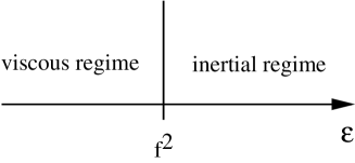
Figure 4: Viscous and inertial regimes, thick layer; $f=(l_{v}/l_{c})^{3/2}$ and $\varepsilon=\Phi-1$.

As seen above, the cross-over between the inertial and the viscous regime appears when $\varepsilon=f^{2}$ where $\varepsilon\ll 1$ (Figure 4). This relation yields the following consequences:
$\bullet$ Strictly at the onset of instability ($\varepsilon=0$), the condition of inertial regime is never reached: the ferrofluid has a viscous behaviour ($f$ is finite).
$\bullet$ By increasing the magnetic induction, we reach the inertial regime above $\varepsilon=f^{2}$ (while keeping $\varepsilon\ll 1$).
For example, with the ferrofluid APG 512 A ($f\simeq 0.27$), the inertial regime takes place when $H_{0}\simeq H_{crit}^{thick}(1+\frac{\varepsilon}{2})=H_{crit}^{thick}(1+\frac{f^{2}}{2})$ i.e. $H_{0}\simeq 1.04~{}H_{crit}^{thick}$.
In Table 3, we present different values of the parameter $f$. With the ferrofluid EMG 507, the inertial regime is reached when $H_{0}\simeq 1.00002~{}H_{crit}^{thick}$: we can then consider that the description thick-inertial is adequate, whatever $H_{0}$ is.
It appears then, that the regime viscous or inertial, near the onset, depend on the type of ferrofluid. One also could use a ferrofluid, for example APG 067 or APG 314, that enables to remain in the viscous regime far enough from the onset. Physical data of various ferrofluids are presented in Table 5.

4.2 Thin film

It seems obvious that the thick case is easier to experiment than the thin case. In order to stick to an opinion, the typical ferrofluid APG 512 A has a capillary length $l_{c}\simeq 1.7$ mm so that for the thin regime, the condition $a\ll l_{c}$ is quite difficult to experiment. The thin regime could be easier to attain if we could increase $l_{c}$ and this may be achieved under microgravity conditions. Typical conditions of microgravity experiments lead to a value of $10^{-2}~{}g$ ($1~{}g=9.81$ m/s²) in parabolic flys [18] ($l_{c}\simeq 17$ mm) and $10^{-6}~{}g$ in orbital stations [19] ($l_{c}\simeq 1.7$ m). In order to make an experiment, one can choose a value of $g$ that enables to have a value of $l_{c}$ large enough but not too much (the distance between the peaks is also proportional to $l_{c}$). Brand and Pettit made an experiment with a 8 mm deep layer on a parabolic fly [20] (As the capillary length of their ferrofluid is $l_{c}=15.5$ mm in the low gravity phase of the parabolic fly, they were not actually in thin nor thick regime).

4.2.1 Thin-inertial film

If the Reynolds number $Re\gg 1$ i.e. $\frac{|s|a^{2}}{f}\gg 1$, we obtain the following equation:

$$s^{2}=a(-k^{4}+2\Phi k^{3}\left(\frac{1+\mu_{o}/\mu}{2}\right)-k^{2})$$ (6)

Let us consider the function $c(\mu)=\frac{1+\mu_{0}/\mu}{2}$, where $c(\mu)\leq 1$. At the onset of the instability, $\Phi=\frac{2}{1+\mu_{o}/\mu}$ ($\geq 1$) and $k_{crit}=1$. When $\Phi\geq\frac{2}{1+\mu_{o}/\mu}$, the wavenumber of maximum growth rate is given by:

$$k_{m}=\frac{1}{4}(3\Phi c+\sqrt{9\Phi^{2}c^{2}-8})$$

The asymptotic critical magnetic induction in the thin case is different from the one of the thick case and always larger. In order to quantify this difference, we have to solve implicit equations in section (5).
We denote $\varepsilon$ as $\varepsilon=\Phi c-1$. Near the onset of instability, the growth rate can be developed, at lowest order in $\varepsilon$ and $\delta k$, and leads to:

$$s^{2}(\Phi c=1+\varepsilon,k=k_{crit}+\delta k)=s^{2}(\varepsilon,\delta k)=a(2\varepsilon-\delta k^{2})$$

We obtain then that $s^{2}$ has the order of magnitude $a\varepsilon$.

The validity conditions are:

$$\left\{\begin{array}[]{lrc}a\ll 1&\mbox{(thin film)}\\ f^{2}/a^{5}\ll\varepsilon&\mbox{(inertial film)}\end{array}\right.$$

4.2.2 Thin-viscous film

When the Reynolds number $Re\ll 1$ i.e. $\frac{|s|a^{2}}{f}\ll 1$, the equation (3) becomes [12]:

$$s=\frac{a^{3}}{3f}(-k^{4}+2\Phi k^{3}(\frac{1+\mu_{o}/\mu}{2})-k^{2})$$ (7)

At the onset of the instability, $\Phi=\frac{2}{1+\mu_{o}/\mu}$ and $k_{crit}=1$. When $\Phi\geq\frac{2}{1+\mu_{o}/\mu}$, the wavenumber of maximum growth rate is given by:

$$k_{m}=\frac{1}{4}(3\Phi c+\sqrt{9\Phi^{2}c^{2}-8})$$

Near the onset, we develop the growth rate in $\varepsilon$ and $\delta k$:

$$s(\Phi c=1+\varepsilon,k=k_{crit}+\delta k)=(a^{3}/3f)(2\varepsilon-\delta k^{2})$$

or also $s$ of order of magnitude $(a^{3}/f)\varepsilon$.
The validity conditions are:

$$\left\{\begin{array}[]{lrc}a\ll 1&\mbox{(thin film)}\\ f^{2}/a^{5}\gg\varepsilon&\mbox{(viscous film)}\end{array}\right.$$

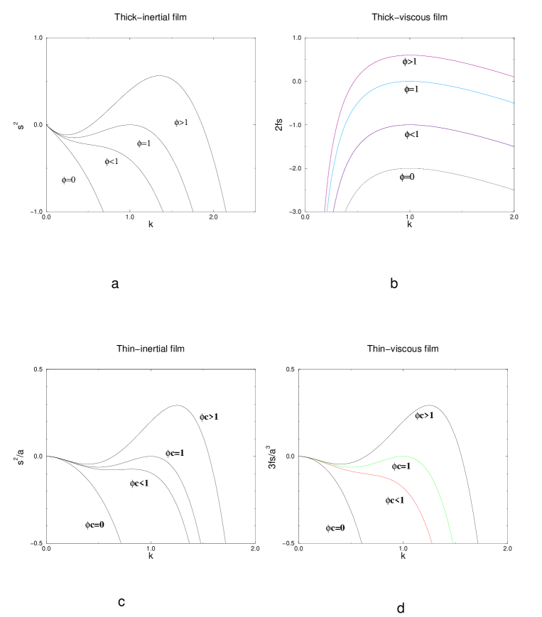
Figure 3: The dispersion relations: ${\bf a}$: $k_{m}$ depends on $\Phi$; $k_{crit}=1$; $\Phi_{crit}=1$. ${\bf b}$: $k_{m}=k_{crit}=1$; $\Phi_{crit}=1$. ${\bf c},{\bf d}$: $k_{m}$ depends on $\Phi$; $k_{crit}=1$; $\Phi_{crit}=1/c=\frac{2}{1+\frac{\mu_{0}}{\mu}}$.

The dispersion relations of the different cases are presented on Figure 3.

4.2.3 Near the onset of the instability

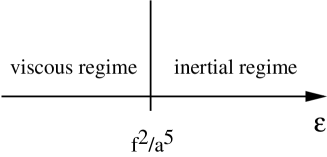
Figure 5: Viscous and inertial regimes, thin layer; $f=(l_{v}/l_{c})^{3/2}$, $\varepsilon=\Phi c-1$ and $a$ is the layer thickness.

In the thin case, we can notice that:
$\bullet$ At the onset of the instability, the thin film of ferrofluid has a viscous behaviour.
$\bullet$ The cross-over to the inertial regime is reached when $\varepsilon=f^{2}/a^{5}$ (Figure 5).
In the case of a thin layer, $\frac{1}{a^{5}}$ tends to $0$: it results in the fact that a thin film has a viscous behaviour, at the onset and far above. With the ferrofluid EMG 507 ($f\simeq 0.0068$), we reach the inertial regime when $H_{0}\simeq H_{crit}^{thin}(1+\frac{\varepsilon}{2})=H_{crit}^{thin}(1+f^{2}/(2a^{5}))$ i.e. $H_{0}\simeq 3~{}H_{crit}^{thin}$ ($a=0.1$).

5 Implicit equations for the asymptotic critical fields

As the magnetic permeability depends on the magnetic field, each asymptotic value of the critical magnetic induction (thick or thin) satisfies an implicit equation.
$\bullet$ In the thick case, the onset is given by equations (2): it is then necessary to know $\mu_{r}(H=H_{crit}^{thick})$ to calculate the critical values. In calculations of section (3), the function $\mu_{r}(H)$ is a constant equal to $\mu_{r}(H_{crit}^{thick})$ (since our linear approach is valid near the onset). This leads to the implicit equation: $H_{crit}^{thick}=f(\mu_{r}(H_{crit}^{thick}))\sqrt{2/\mu_{0}}(\rho g\gamma)^{1/4}$ where $f(\mu_{r})=\frac{\sqrt{1+1/\mu_{r}}}{\mu_{r}-1}$. The function $f(\mu_{r})$ i.e. $H_{crit}^{thick}$ varies rapidly as a function of $\mu_{r}$.
$\bullet$ In the thin case, the implicit equation can be written:

$$H_{crit}^{thin}=\sqrt{\frac{2}{1+\frac{1}{\mu_{r}(H_{crit}^{thin})}}}~{}H_{crit}^{thick}$$ (8)

where $\mu_{r}$ is the relative permeability of the ferrofluid. $H_{crit}^{thick}$ is determined by the equation (2) but note that in equation (8), $H_{crit}^{thick}$ is a constant.
The question arises as to when we can reach the asymptotic value $\sqrt{2}$ of the ratio $H_{crit}^{thin}/H_{crit}^{thick}$ in order to put easily in evidence experimentally the difference between the asymptotic values of the critical magnetic inductions. The Langevin’s classical theory has been adapted to yield the superparamagnetic magnetization relationship between the applied field $H_{0}$ and the resultant magnetization $M$ of the particle collection. For a colloidal ferrofluid composed of particles of one size, we have:

$$M=M_{sat}\left(\coth(\alpha)-\frac{1}{\alpha}\right)\equiv L(\alpha)$$ (9)

whith $\alpha=\frac{mH_{0}}{\it{k}T}$, where $m$ is the magnitude of the magnetic moment of a particule, $L$ is the Langevin function, $M_{sat}$ the saturation moment of the ferrofluid and $\it{k}$ the Boltzmann constant. When the initial permeability is appreciable, it is no longer permissible to neglect the interaction between the magnetic moments of the particles ([22], [23], [24]) and equation (9) has to be modified. We shall consider equation (9) as a good first approximation (while $\chi_{i}$ is not much larger than unity). This leads to the expression of the relative magnetic permeability:

$$\mu_{r}(H_{0})=1+\frac{M_{sat}}{H_{0}}L\left(3\frac{H_{0}}{M_{sat}}\chi_{i}\right)$$ (10)

This function of $H$ decreases from $\mu_{r}(0)=\chi_{i}+1$ to $1$. With the ferrofluid APG 512 A ($\chi_{i}=1.4$), solving the implicit equations (2) and (8) results in $H_{crit}^{thick}=65.2$ Gauss and $H_{crit}^{thin}=77.0$ Gauss. The ratio $H_{crit}^{thin}/H_{crit}^{thick}=1.18$ and the difference $H_{crit}^{thin}-H_{crit}^{thick}=11.8$ Gauss. Table 4 presents other ferrofluids results: We note that the ratio $H_{crit}^{thin}/H_{crit}^{thick}$ increases and the difference $H_{crit}^{thin}-H_{crit}^{thick}$ decreases as $\chi_{i}$ increases. It is better to use a ferrofluid with a low value of $\chi_{i}$ to put experimentally in evidence the difference between $H_{crit}^{thin}$ and $H_{crit}^{thick}$.

6 Conclusion

We get the dispersion relation of a layer of magnetic fluid of any thickness and viscosity, under a uniform vertical magnetic field. The critical magnetic field and the critical wavenumber of this instability are found to be thickness-dependent. The dispersion equation, simplified into four asymptotic regimes, enables to explicit the expression of the critical magnetic induction of a thin film of ferrofluid. Near the onset of the instability, we show that the behaviour of the ferrofluid may be viscous or completely inertial; the behaviour which is manifested depends on the characteristics of the ferrofluid (contained in the parameter $f$ proportional to $\nu$). In order to put in evidence experimentally the fact that the critical magnetic induction depends on the thickness, it is better to use a ferrofluid with a low value of the initial susceptiblity $\chi_{i}$.

7 Acknowledgement

Philippe Claudin is gratefully acknowledged for fruitful discussions. Ferrofluidics Corporation, and in particular Karim Belgnaoui, are acknowledged for help in collecting physical data (Table 5) of the ferrofluids they propose.

Figure 1: Curve of marginal stability; thick-inertial layer.

Figure 2: Ferrofluid layer in the vacuum and in a magnetic induction.

	$\mbox{Re}\ll 1$	$\mbox{Re}\gg 1$
$a/l_{x}\ll 1$	thin-viscous regime: $\mbox{Re}=\frac{|s|a^{2}}{\nu}$	thin-inertial regime: $\mbox{Re}=\frac{|s|a^{2}}{\nu}$
$a/l_{x}\gg 1$	thick-viscous regime: $\mbox{Re}=\frac{|s|}{2\nu k^{2}}$	thick-inertial regime: $\mbox{Re}=\frac{|s|}{2\nu k^{2}}$

Table 1: The asymptotic regimes

capillary length	$l_{c}=(\gamma/\rho g)^{1/2}$
capillary time	$t_{c}=(l_{c}/g)^{1/2}$
capillary Laplace pressure	$p_{c}=\gamma/l_{c}$

Table 2: Capillary quantities

ferrofluid	$f$	$H_{0}/H_{crit}^{thick}$ when begins the inertial regime
EMG 507	0.0068	1.00002
EMG 901	0.039	1.0008
APG 512 A	0.27	1.04
APG 314	0.71	1.25
APG 067	1.29	1.8

Table 3: Range of the viscous and inertial regimes in the thick case

ferrofluid	EMG 308	APG 512 A	EMG 900
$\chi_{i}$	0.3	1.4	4.2
$M_{sat}$ (Gauss)	600	300	900
$H_{crit}^{thick}$ (Gauss)	299.5	65.2	19.7
$H_{crit}^{thin}$ (Gauss)	318.2	77.0	25.5
$H_{crit}^{thin}/H_{crit}^{thick}$	1.06	1.18	1.29
$H_{crit}^{thin}-H_{crit}^{thick}$ (Gauss)	18.7	11.8	5.8

Table 4: Critical characteristics of various ferrofluids

ferrofluid	$\rho$ (g/cm3)	$\gamma$ (N/m)	$\eta$ (mPa s)	$\chi_{i}$
EMG 507	1.15	$\sim$ 0.033	2	0.4
EMG 900	1.74	0.025	60	4.2
EMG 308	1.05	$\sim$ 0.04	5	0.3
EMG 901	1.53	0.0295	10	3
APG 512 A	1.26	0.035	75	1.4
APG 314	$\sim$ 1.2	0.025	150	1.2
APG 067	1.32	0.034	350	1.4

Table 5: Physical data of ferrofluids (Ferrofluidics Corporation).

References

- [1] M. D. Cowley and R. E. Rosensweig. The interfacial stability of a ferromagnetic fluid. J. Fluid Mech., 30(4):671–688, 1967.
- [2] R. E. Rosensweig. Ferrohydrodynamics. Cambridge Univ. Press, 1985.
- [3] A. Gailitis. Formation of the hexagonal pattern on the surface of a ferromagnetic fluid in an applied magnetic field. J. Fluid Mech., 82:401–413, 1977.
- [4] H. Herrero, C. Perez-Garcia, and M. Bestehorn. Stability of fronts separating domains with different symmetries in hydrodynamical instabilities. Chaos, 4(1):15–20, March 1994.
- [5] H. Brand and J. E. Wesfreid. Phase dynamics for pattern-forming equilibrium systems under an external constraint. Phys. Rev. A, 39(6):6319–6322, 1989.
- [6] G. Taylor and A. D. McEwan. The stability of a horizontal fluid interface in a vertical electric field. J. Fluid Mech., 22:1–15, 1965.
- [7] T. P. Hynes. Stability of thin films. PhD thesis, Churchill College, Cambridge, 1978.
- [8] L. Limat. Instabilité d’un liquide suspendu sous un surplomb solide: influence de l’épaisseur de la couche. C. R. Acad. Sci. Paris, 317(2):563–568, 1993.
- [9] G. Néron de Surgy, J. P. Chabrerie, O. Denoux, and J. E. Wesfreid. Linear growth of instabilities on a liquid metal under normal electric field. J. Phys. II (Paris), 3:1201–1225, 1993.
- [10] J. Weilepp and H.R. Brand. Competition between the Bénard-Marangoni and the Rosensweig instability in magnetic fluids. J. Phys. II (Paris), 6:419–441, 1996.
- [11] Salin D. Wave vector selection in the instability of an interface in a magnetic or electric field. Europhys. Lett., 21(6):667–670, 1993.
- [12] Bacri J. C., Perzynski R., and Salin D. Instabilité d’un film de ferrofluide. C. R. Acad. Sci. Paris, 307(II):699–704, 1988.
- [13] J. E. Wesfreid and S. Zaleski. Cellular structures in instabilities. Springer-Verlag, 1983.
- [14] D. Allais and J. E. Wesfreid. Bull. Soc. Fr. Phys. Suppl., 57:20, 1985.
- [15] U. d’Ortona, J. C. Bacri, and D. Salin. Magnetic fluid oscillator: observation of nonlinear period doubling. Phys. Rev. Lett., 67:50–53, 1991.
- [16] Landau L. D. and Lifshitz E. R. Fluid Mechanics. Pergamon Press, New York, 1958.
- [17] in preparation.
- [18] J.-B. Renard. L’impesanteur en caravelle zéro-G. In Revue du palais de la découverte, volume 23. May 1995.
- [19] M. Nati and M. Bandecchi. Esa ready to contribute to the microgravity-environment monitoring of the space station. In Microgravity news from ESA, volume 8. August 1995.
- [20] D. R. Pettit and H. R. Brand. On the influence of near zero gravity on the Rosensweig instability in magnetic fluids. Phys. Lett. A, 159:55–60, 1991.
- [21] When in equation (6), we expect to find the corresponding dispersion equation of electric case. This is not right: we have to consider the equation where . We check that if , and we obtain the electrical case [9]. This equation leads to (6) after the following simplifications: , , so that we can’t consider in equation (6).
- [22] M. I. Shliomis. Magnetic Fluids. Sov. Phys. Usp., 17(2):153–169, 1974.
- [23] R. Kaiser and G. Miskolczy. Magnetic properties of stable dispersions of subdomain magnetic particles. J. Appl. Phys, 41(3):1065–1072, 1970.
- [24] C. P. Bean and J. D. Livingston. Superparamagnetism. J. Appl. Phys, 30(4):120S–129S, 1959.