STABILITY AND HALO FORMATION
IN AXISYMMETRIC INTENSE BEAMS

Abstract

Beam stability and halo formation in high-intensity axisymmetric 2D beams in a uniform focusing channel are analyzed using particle-in-cell simulations. The tune depression - mismatch space is explored for the uniform (KV) distribution of the particle transverse-phase-space density, as well as for more realistic ones (in particular, the water-bag distribution), to determine the stability limits and halo parameters. The numerical results show an agreement with predictions of the analytical model for halo formation [1].

I Introduction

There is an increasing interest in high-current applications of ion linacs, such as the transformation of radioactive waste, the production of tritium, and fusion drivers. High currents of the order of 100 mA restrict beam losses below 1 ppm. Thorough studies are necessary to understand mechanisms of intense-beam losses, in particular, beam instabilities and halo formation.

Most of the theoretical efforts so far have concentrated on the Kapchinsky-Vladimirsky (KV) distribution of particles in transverse phase space [2]. The KV beam density is uniform so that space-charge forces inside the beam are linear. It allows an analytical investigation and results are used to predict the behavior of real beams. On the other hand, it is recognized that the KV model, in which all particles have the same transverse energy, is not a realistic beam distribution, e.g. [3]. The present paper compares the KV beam with other, nonlinear particle-density distributions, which can serve as better models for real beams.

II Analytical Consideration

We study a continuous axisymmetric ion beam in a uniform focusing channel, with longitudinal velocity $v_{z}=\beta c$. The Hamiltonian of the transverse motion ($v_{\bot}\ll v_{z}$) is

$$H(r,s)=s^{2}/2+k_{0}^{2}r^{2}/2+q\Phi(r)/(m\gamma^{3}\beta^{2}c^{2})\ ,$$ (1)

where $m$ and $q$ are ion mass and charge, $k_{0}$ is the focusing strength of the channel, $\gamma=(1-\beta^{2})^{-1/2}$, $r=\sqrt{x^{2}+y^{2}}$ is the distance from the $z$-axis in the transverse plane, and $s=\sqrt{x^{\prime 2}+y^{\prime 2}}$ ($x^{\prime}=\dot{x}/\beta c$, $y^{\prime}=\dot{y}/\beta c$) is the dimensionless transverse velocity. The electric potential $\Phi(r)$ must satisfy the Poisson equation

$$\nabla^{2}\Phi(r)=-(q/\varepsilon_{0})\int\!\!\int d\vec{s}f(r,s)\ ,$$ (2)

where $f(x,y,x^{\prime},y^{\prime})=f(r,s)$ is the distribution function in the transverse non-relativistic 4-D phase space. The integral on the RHS is the particle density $d(r)$.

Since the Hamiltonian (1) is an integral of motion, any distribution function of the form $f(r,s)=f(H(r,s))$ is a stationary distribution. We consider a specific set of stationary distributions for which the beam has a sharp edge (for all ions $r\leq r_{max}=a$), namely,

$$f_{n}(H)=\left\{\begin{array}[]{cc}N_{n}n(H_{0}-H)^{n-1}&\mbox{for }H\leq H_{0}\ ,\\ 0&\mbox{for }H>H_{0}\ .\end{array}\right.$$ (3)

The normalization constants $N_{n}$ are chosen to satisfy $2\pi\int_{0}^{a}rdrd(r)=I$, where $d(r)$ is the particle density, and $I$ is the beam current. The set includes the KV distribution, $f_{0}=N_{0}\delta(H_{0}-H)$, as a formal limit of $n\to 0$, as well as the waterbag (WB) distribution, $f_{1}=N_{1}\theta(H_{0}-H)$, where $\theta(x)$ is the step-function. For a detailed discussion of these two specific examples see [4].

We introduce the function $G(r)=H_{0}-H(r,s)+s^{2}/2$, because the density can be expressed from (3) as $d(r)=2\pi N_{n}G^{n}(r)$. Physically, this function gives the maximal transverse velocity for a given radius, $s_{max}(r)=\sqrt{2G(r)}$, and defines the boundary in the phase space $(r,s)$. It allows us to rewrite Eq. (2) as

$$\left[rG^{\prime}(r)\right]^{\prime}/r-\lambda^{2}G^{n}(r)=-2k_{0}^{2}\ ,$$ (4)

with boundary conditions $G(a)=0$, and $G(0)\equiv G_{0}$ is finite. Here the parameter $\lambda^{2}=K/\left[\int_{0}^{a}rdrG^{n}(r)\right]$, where $K=2I/\left(I_{0}\beta^{3}\gamma^{3}\right)$ is the beam perveance, and $I_{0}=4\pi\varepsilon_{0}mc^{3}/q$ is a constant. Particular solutions to (4) are easy to find for $n=0$ (KV) and $n=1$ (WB) [4]. For $n\geq 2$ a numerical solution is required.

To compare different transverse distributions on a common basis, we consider rms-equivalent beams which have the same perveance $K$, rms radius, and rms emittance $\tilde{\mathcal{E}}$. To characterize the space-charge strength, one introduces an equivalent (or rms) tune depression

$$\eta=\sqrt{\,1-K/(4k_{0}^{2}x^{2}_{rms})}\ ,$$ (5)

which reduces to the usual one for the KV beam. For numerical simulations we use dimensionless variables: $\hat{z}=k_{0}z$, and $\hat{x}=x\sqrt{k_{0}/\mathcal{E}}$, where ${\mathcal{E}}=a^{\prime}a$. In normalized variables the beam matched radius is $\hat{a}=\sqrt{(C_{\mathcal{E}}/C_{2})/\eta}$, where $C_{\mathcal{E}}=\tilde{\mathcal{E}}/\mathcal{E}$ and $C_{2}=x^{2}_{rms}/a^{2}$. For the KV case, $C_{\mathcal{E}}=C_{2}=1/4$, so that $\hat{a}=1/\sqrt{\eta}$. The “hats” are omitted below to simplify notation.

III Numerical Simulations

We use particle-in-cell simulations to study beam stability and halo formation in the presence of instabilities. A leap-frog integration is applied to trace the time evolution for a given initial phase-space distribution. The space-charge radial electric field of an axisymmetric beam can be found from Gauss’ law by counting the numbers of particles in cells of a finite radial grid, which extends up to four times the beam matched radius. The initial phase-space state is populated randomly but in accordance with (3) for a chosen $n$. The matched distributions remain stable except for a minor dilution related to numerical errors. However, even the matched KV beam is unstable for $\eta\leq 0.4$, in agreement with existing theory [5] and earlier simulations [6].

The beam breathing oscillations are excited by loading a mismatched initial distribution $r_{i}=\mu\tilde{r}_{i}$, $r^{\prime}_{i}=\tilde{r}^{\prime}_{i}/\mu$, where $\tilde{r}_{i},\tilde{r}^{\prime}_{i}$ correspond to the matched one, and the mismatch parameter $\mu\leq 1$. A typical range of the simulation parameters: time step $\Delta t=T/100$, where $T$ is the period of breathing oscillations, total number of particles $N_{par}=16K\mbox{ to }4096K$, where $K=1024$, and radial mesh size $\Delta r=a/128\mbox{ to }a/16$. The code performs simulations of about 100 breathing oscillations per CPU hour for $N_{par}=256K$ on Sun UltraSparc 1/170.

The beam behavior is studied as a function of tune depression $\eta$ and mismatch $\mu$. Due to a discrete filling of a mismatched beam distribution in simulations and, for $n\geq 1$, due to non-linear space-charge forces, higher modes are excited in addition to the breathing mode. Some of them can be unstable depending on values of $\eta$ and $\mu$. A detailed numerical study of stability and halo formation for the KV beam and its comparison with the theory predictions [5, 1] have already been reported in [7, 8]. Here we compare results for different transverse distributions. In Figs. 1-2 the maximal radius of the whole ensemble of particles is plotted versus the number of breathing oscillations for the KV and WB beams, for the particular case of $\eta=0.7$ and $\mu=0.8$ ($N_{par}=256K$, $\Delta r=a/64$).

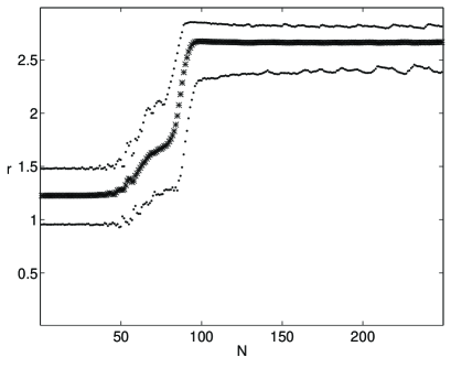
FIG. 1.: KV beam radius versus the number of breathing periods for $\eta=0.7$ and $\mu=0.8$. Stars are for period averages, dots show minimum and maximum during a period.

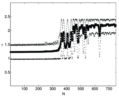
FIG. 2.: The same as Fig. 1, but for the WB beam.

Comparison of Figs. 1 and 2 shows that for these parameters the WB beam remains stable much longer than the KV one, but eventually it also blows up and some particles form a halo far from the beam core. Results for the $n=2$ distribution are similar to those for WB. Some results depend on simulation parameters; e.g., it takes a smaller number of the breathing periods for a beam to blow up if $N_{par}$ is smaller (i.e., higher noise). However, the maximum radius, as well as the fraction of particles outside the core, are practically independent of $N_{par}$. The number of particles which go into the halo and produce jumps of $r_{max}$ seen in Figs. 1-2, might be rather small. We define the halo intensity $h$ as the number of particles outside the boundary $r_{b}=1.75a$ divided by $N_{par}$. Such a definition is arbitrary, but convenient to compare beam halos over a wide range of tune depressions. While the beam behavior in Figs. 1 and 2 seems qualitatively similar, the halos for these two cases are very different: $h\simeq 3.5\cdot 10^{-3}$ for KV, and about 100 times less for the WB, with only a few particles in the halo (less than 10 of 256K). That is the reason for oscillations of $r_{max}$ in Fig. 2: these few halo particles can initially all come back to the core simultaneously.

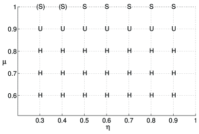
FIG. 3.: Beam behavior (qualitatively) versus tune depression $\eta$ and mismatch $\mu$.

A qualitative picture of the beam behavior for various values of the tune depression and mismatch is shown in Fig. 3, and is practically the same for all distributions studied. ’H’ corresponds to beam instability with halo formation, usually with a noticeable emittance growth, ’U’ means that the beam is unstable but a halo is not observed in our simulations, and ’S’ indicates beam stability. The most surprising feature of the diagram is the lack of any significant dependence on $\eta$ for mismatched beams; on the contrary, the qualitative changes depend primarily on $\mu$. When $\mu$ changes from 0.6 to 0.8, the ratio $\tilde{\mathcal{E}}_{fin}/\tilde{\mathcal{E}}_{ini}$ decreases from 1.7–2 to 1.03–1.07 for the KV beam, and from 1.4–1.5 to 1.00–1.01 for the WB and $n=2$. The number of breathing periods after which the beam radius starts to grow noticeably and the halo forms, has some dependence on $\eta$; it is smaller for small $\eta$.

We performed a systematic study of the KV, WB, and $n=2$ distributions for tunes $\eta$ from 0.1 to 0.9 and mismatches $\mu$ from 0.6 to 1.0. Figure 4 shows the ratios of the halo radius to that of the matched beam for the KV and WB beams with three different mismatches, $\mu=0.6$, 0.7, and 0.8. Results for $n=2$ beam are not shown; they are slightly lower than those for the WB beam. The KV halo has a larger radius, especially with small space charge (large $\eta$), but for space-charge dominated beams, at very small $\eta$, the ratios converge for all distributions. The analytical model for the KV halo formation [1] predicts finite values of $r_{max}/a$ between 2 and 2.5 depending on $\eta$ and $\mu$. One can see from simulations that it works well also for WB and $n=2$ beams.

FIG. 4.: Ratio of halo radius to that of the matched beam for KV (top curves) and WB (bottom curves) beams versus tune depression $\eta$ for different mismatches: $\mu=0.6$ long-dashed, $\mu=0.7$ short-dashed, $\mu=0.8$ dotted.

Simulation results for halo intensity $h$ are shown in Fig. 5 for KV and WB distributions. Again, results for $n=2$ are just slightly lower than for the WB beam, and not shown. The intensity depends essentially on the mismatch, and decreases quickly as the mismatch decreases. The WB halo is about 2–3 times less intense than the KV halo for small space charge and large mismatch (0.6 and 0.7) but, for space-charge dominated beams, the intensities are about the same. For $\mu=0.8$, however, the WB halo is at least an order of magnitude less intense than the KV one; it is not even included in Fig. 5. An apparent decrease of $h$ as $\eta$ decreases is due to the definition used: the halo boundary radius $r_{b}=1.75a$ increases as $1/\sqrt{\eta}$. If a fixed boundary is used instead, the same for all tunes, the halo intensity would be larger for larger space charge.

FIG. 5.: Halo intensity for KV (solid) and WB beams (dashed) vs tune depression $\eta$ for mismatches $\mu=0.6$ (top pair), $\mu=0.7$ (middle pair), $\mu=0.8$ (bottom, KV only).

One more interesting feature is how fast the halo develops. For the KV beam, the process is usually rather fast, and the halo saturates after a few hundred breathing periods. For the WB and $n=2$ distributions, it continues to grow rather slowly, and asymptotic values are usually reached after a few thousand breathing oscillations; it takes especially long for $\eta\leq 0.3$. Data plotted in Fig. 5 correspond to the asymptotic values, after N=5000 breathing periods for WB and after N=600 for KV (except $\eta\leq 0.2$, where KV results are also for N=5000). These 5000 breathing oscillations correspond to 5–10 km of the length for a typical machine, much longer than existing proton linacs.

IV Conclusions

Our simulations show the qualitative similarity of the beam behavior for all transverse distributions studied. The KV beam can be considered as an extreme case compared to the WB and $n=2$ distributions which are closer to real beams. The halo intensity is a few times higher and saturates faster for the KV distribution than for the other two.

An interesting new observation is that for axisymmetric beams under consideration the beam stability and halo formation depend primarily on the mismatch, not on the tune shift. The halo was clearly observed only for large mismatches, at least 20%, and its radius is in agreement with the analytical model [1] for halo formation.

REFERENCES

- [1] R.L. Gluckstern, Phys. Rev. Letters 73, 1247 (1994).
- [2] I.M. Kapchinsky and V.V. Vladimirsky, in Proceed. Int. Conf. on High Energy Accelerators (CERN, Geneva, 1959), p. 274.
- [3] H. Okamoto and M. Ikegami, Phys. Rev. E 55, 4694 (1997).
- [4] M. Reiser, Theory and Design of Charged Particle Beams (Wiley, New York, 1993).
- [5] R.L. Gluckstern, in Proceed. of the Linac Conference (Fermilab, 1970), p. 811.
- [6] I. Hofmann, L.J. Laslett, L. Smith and I. Haber, Particle Accelerators 13, 145 (1983).
- [7] R.L. Gluckstern, W.-H. Cheng and H. Ye, Phys. Rev. Letters 75, 2835 (1995).
- [8] R.L. Gluckstern, W.-H. Cheng, S.S. Kurennoy and H. Ye, Phys. Rev. E 54, 6788 (1996).