A soluble model of evolution and extinction dynamics in a rugged fitness landscape.

Abstract

We consider a continuum version of a previously introduced and numerically studied model of macroevolution [2], in which agents evolve by an optimization process in a rugged fitness landscape and die due to their competitive interactions. We first formulate dynamical equations for the fitness distribution and the survival probability. Secondly we analytically derive the $t^{-2}$ law which characterizes the life time distribution of biological genera. Thirdly we discuss other dynamical properties of the model as the rate of extinction and conclude with a brief discussion.

87.10.+e,02.50.f2,05.40.+j,03.20.+i

Aspects of evolution and extinction can be described as emergent behavior in a large set of interacting agents[2, 3, 4, 5], moving stochastically in a rugged fitness landscape[6]. The behavior of the models of Refs.[3, 4, 5] stems from fluctuations in a time homogeneous stochastic process. This agrees with a commonly held perception, e.g. implied when a birth-death process with constant rates[7] is used to fit survivorship data and when the size of extinction events is presented as a ‘kill curve’[8]. A quite different paradigm is also frequently met in the literature: Raup and Sepkoski [9] noted that the apparent decrease of the extinction rate through geological times could be ‘… predictable from first principles if one argues that general optimization of fitness through evolutionary time should lead to prolonged survival ’. Gould[10] uses an unexpected source of statistical data to illustrate evolutionary non-homogeneity as it reveals itself in the ‘unreversed, but constantly slowing, improvement in mean fielding average through the history of baseball’. Concurring observations from experimental studies of bacterial evolution in a constant environment can be found in Ref.[11] as well as from numerical experiments on the ‘long jump dynamics’ of the NK model in Ref.[12].

In this Letter we consider stochastic evolution in a rugged fitness landscape. The assumptions are the same in spirit as those of a previously introduced and numerically studied ‘reset’ model[2]. However, they are here expressed in a further simplified way, allowing a (mainly) analytical rather than (mainly) numerical treatment, and leading to close form expressions for the survivorship curves and life span distributions, which are of general interest in the study of complex evolving systems, biological or not. We use two – somewhat extreme – assumptions in line with a non-stationary evolution paradigm: Firstly, the progeny of individual mutants less fit than the currently dominating genotype never establish itself within the population. Then, as a macroscopic evolutionary step can only be triggered by a fitness record within the population, the current typical genotype always codes the best solution found ‘so far’. Secondly, competitive interactions among species depend on fitness in a non-symmetric way, as evolving species only kill their less fit neighbors. The predictions of the present model resemble the behavior of the reset model and are in good agreement with empirical data describing biological genera [7, 8, 13, 14, 15, 16].

In the sequel we first derive equations for the fitness distribution of the system $P(x,t)$ and for the probability $W_{t}(\tau)$ that a tagged species born at time $t$ survive time $\tau$. We then analytically find the $\tau^{-1}$ dependence of $W$ and the ensuing $\tau^{-2}$ dependence of the life-time distribution $R_{t}(\tau)$. Next we discuss the parametric $t$ dependence which is not in general analytically available, the effect of averaging over $t$, and the long time asymptotic behavior of $P(x,t)$ for different parameter values. We conclude by with a brief assessment of the robustness of the model.

To construct a dynamical equation for $P(x,t)$ we proceed in two steps, starting with the limiting case where no extinctions take place and where, as a consequence of hill climbing in a random fitness landscape, a suitably defined[2, 17, 18] average fitness grows logarithmically:

$$D(t)=\log(t+1).$$ (1)

With no interactions, an initial fitness distribution would be rigidly shifted in (log) time. As $D$ solves the equation of motion $v(x)=dx/dt=\exp(-x)$ with initial condition $D(0)=0$, the time evolution of a distribution of non interacting agents $P(x,t)$ solves the transport equation: $\partial P(x,t)/\partial t+\partial(v(x)P(x,t))/\partial x=0.$ Interactions enter via an additional term $-gP(x,t)K(P(x,t))$, where $K$ is an effective killing rate and where the constant $g$ describes what fraction of the system is affected by an evolutionary event.

Species going extinct vacate a niche, which is refilled at a later time. This in and outflow is expediently accounted by introducing a ‘limbo’ state, which absorbs extinct species, and from which new species emerge at the low fitness boundary of the system. A finite upper bound to the total number of species which can coexist implies a conservation law : $N(t)+\int_{0}^{\infty}P(y,t)dy=1$. With the chosen normalization $N(t)$ is the fraction of species in the limbo state, while $P(x,t)$ is the probability density of finding a living species with fitness $x$. The above considerations lead us to the differential equations:

$$\frac{dN(t)}{dt}=-bN(t)+g\int_{0}^{\infty}P(z,t)K(P)dz$$ (2)

$$\frac{\partial P(x,t)}{\partial t}=-\frac{\partial(v(x)P(x,t))}{\partial x}-gP(x,t)K(P)$$ (3)

where $b$ is the rate at which species are generated at the low fitness end of the system. The corresponding initial and boundary conditions are: $N(t=0)=N_{0},\;\forall x:P(x,t=0)=P_{0}(x),\;\forall t:\int_{0}^{\infty}P(x,t)dx=1-N(t)<\infty,\;$ and finally $\forall t:P(x=0,t)=bN(t)$.

We consider below a form of the killing rate $K$ which is as close as possible to the reset model: The killing at fitness $x$ is taken to depend on the rate of evolutionary change of agents with fitness larger than $x$: low-fitness agents suffer if high fitness agents evolve - but not vice versa. This leads to

$$K(v(x)P(x,t))=(-\int_{x}^{\infty}\partial(vP)/\partial x)^{\alpha}dx=(v(x)P(x,t))^{\alpha},$$ (4)

simply expressing the killing rate as the evolutionary current raised to a power. The exponent $\alpha$ just introduced allows more generality without unduly complicating the analysis: It accounts in a simplified way for possible (spatial) correlations effects in a model where information about individual species is retained. If $\alpha<1$ $(>1)$, a move by an old, slowly evolving species triggers a larger (smaller ) cascade of extinctions than one by a young, fast evolving species. Figure 1 shows six snaphots of the fitness distribution resulting from the above equations, at times equally spaced on a logarithmic scale and for $\alpha=1$, $b=1$ and $g=40$.

A quantity often used to characterize paleontological data is the survivorship curve of a cohort or the closely related life span distribution[7]. In our treatment the former quantity corresponds to the probability $W_{t}(\tau)$ that an agent appearing at time $t$ survive time $\tau$, while the latter can be found from $W_{t}(\tau)$ by differentiation:

$$R_{t}(\tau)=-\frac{dW_{t}(\tau)}{d\tau}.$$ (5)

As an agent born at $t$ and alive at time $t+\tau$ invariably has fitness $D(\tau)=\ln(\tau+1)$ and as the probability of being killed in the interval $d\tau$ is $K(P(D(\tau),t+\tau))d\tau$, $W$ must obey the differential equation:

$$\frac{d\ln W_{t}(\tau)}{d\tau}=-gK(P(D(\tau),t+\tau))\;\;\tau>0,$$ (6)

with initial condition $W_{t}(\tau=0)=1$.

Finally, the model extinction rate is simply the fraction of species which die per unit of time, at time $t$:

$$r(t)=g\int_{0}^{\infty}P(x,t)K(P(x,t))dx=dN/dt+bN.$$ (7)

Note that if $b\rightarrow\infty$, then extinct species are immediately replaced, as in Ref.[2]. Furthermore for any $b$ and large $bt$ $dN/dt$ is negligible and $bN(t)\rightarrow r(t)$ so that the extinction closely balances the inflow.

As a first step towards the solution of Eq.3, we set $q=vP$ and notice that $q$ can be written as $q(z(x,t))$ with

$$dq/dz=-gq^{\alpha+1},$$ (8)

and where $z(x,t)$ satisfies

$$\partial z/\partial t+v(x)\partial z/\partial x=1.$$ (9)

The solution of Eq.8 is simply $q=(\alpha gz)^{-1/\alpha}$. To solve Eq.9 we let $A$ and $B$ be any two functions of a single real variable $x$, which are continuous for $x>0$ and which vanish identically for $x<0$. For $v=\exp(-x)$, the general solution has the form $z(x,t)=\epsilon\exp(x)+(1-\epsilon)t+A(t+1-\exp(x))+B(\exp(x)-(t+1))$ for some constant $\epsilon<1$. Utilizing the initial and boundary conditions, we find $A(y)=(bN(y))^{-\alpha},\;\;y>0$ and $B(y)=(y+1)^{\alpha}P_{0}(\log(y+1))^{-\alpha}-g\alpha y,\;\;y>0,$ leading to

$$P(x,t)=\frac{e^{x}}{\left[g\alpha t+(e^{x}-t)^{\alpha}P_{0}^{-\alpha}(\log(e^{x}-t))\right]^{1/\alpha}}$$ (10)

for $x>D(t)$, while for $x<D(t)$ we have

$$P(x,t)=\frac{e^{x}}{\left[g\alpha(e^{x}-1)+(bN(t+1-e^{x}))^{-\alpha}\right]^{1/\alpha}}$$ (11)

Note that $P$ is continuous in $x$, although its derivative will in general be discontinuous at $x=D(t)$.

The survival probability of a species born at time $t$ (the survivorship curve of a cohort[7]), can be obtained analytically by solving Eq.6. This is so because when inserting $D(\tau)$ in lieau of $x$ in Eq.11, the $\tau$ dependence in the argument of the (unknown) function $N$ drops out. The solution is:

$$W_{t}(\tau)=\left[\frac{(bN(t))^{-\alpha}}{(bN(t))^{-\alpha}+g\alpha\tau}\right]^{1/\alpha}.$$ (12)

As $W$ vanishes for large $\tau$, all species eventually die, regardless of the value of $\alpha$. This behavior is very desirable from a modeling point of view, as it agrees with the fact that by far the largest number of species which ever lived are now extinct [15]. The distribution of life spans can be obtained from Eq.12 by differentiation, as expressed in Eq.5. If $\alpha$ is close to unity, we find a $\tau^{-1}$ behavior for $W_{t}(\tau)$, and hence a $\tau^{-2}$ for $R_{t}(\tau)$, independently of $t$.

Averaging these distributions with respect to $t$ over a time window $T$ is needed if the time of appearance of species is not precisely known, or if data are scarce. Weighing $R_{t}(\tau)$ by the normalized rate at which new species flow into the system we obtain:

$$R(\tau)=\frac{\int_{0}^{T-\tau}N(t)R_{t}(\tau)dt}{\int_{0}^{T}N(t)dt}.$$ (13)

Of course, averaging does not change the behavior significantly if $T$ is short compared to the typical lifetime of the species. In the opposite limit, the behavior is also maintained if $N(t)$ does not not vanish ’too rapidly’ in the limit $t\rightarrow\infty$. To better appreciate this last point, we use Eq.13 in conjunction with Eqs.12 and 5, and express $N^{-\alpha}$ by $W_{t}(\tau)$, obtaining:

$$R(\tau)=g(g\alpha\tau)^{-1-1/\alpha}\frac{\int_{0}^{T-\tau}(1-W_{y}^{\alpha}(\tau))^{1+1/\alpha}dy}{\int_{0}^{T-\tau}bN(y)dy}$$ (14)

Even though this integral cannot be evaluated explicitly, Eq.12 shows that the $\tau$ dependence of the integrand is negligible if the inequality $\alpha g\tau>(bN(y))^{-\alpha}$ holds throughout the integration interval. The $\tau$ dependence stemming from the limits of the integrals can also be ignored for $\tau<<T$. Hence $R\propto\tau^{-1-1/\alpha}$, similarly to the non-averaged case. As shown later, when $\alpha$ close to unity and $g$ sufficiently large, the model yields $r(t)\approx bN(t)\geq t^{-\delta}$ , with $\delta$ close to $0.5$, which means that even though $\tau<<T$ the relation $\tau>T^{\delta\alpha}$ can be fulfilled.

We now restrict ourselves to a limiting case in which $N(t=0)=1$ which is formally at variance with our boundary conditions. However, a limiting process shows that the relevant expression for $P(x,t)$ for $x<D(t)$ remains Eq.11, while $P=0$ for $x>D(t)$. A non-linear equation for $N(t)$ is now obtained by integration of Eq.11, followed by a change of variables. The result is

$$1-N(t)=\int_{0}^{t}\frac{dy}{\left[g\alpha(t-y)+(bN(y))^{-\alpha}\right]^{1/\alpha}}\\$$ (15)

Differentiating Eq.15 with respect to time, and utilizing Eq.7, we find the extinction rate:

$$r(t)=\int_{0}^{t}\frac{g\;dy}{\left[g\alpha(t-y)+(bN(y))^{-\alpha}\right]^{1+1/\alpha}}\\$$ (16)

A closed form solution of these (equivalent) integral equations could not be found in the general case. We notice however a major difference in the asymptotic behavior for $\alpha<1$ and $\alpha\geq 1$. In both cases the time independent function $P_{\infty}(x)$ obtained by taking $t\rightarrow\infty$ and by setting $N(t)=N_{\infty}\neq 0$ in Eq.11 formally satisfies the model equations. However, only for $\alpha<1$ is $P_{\infty}(x)$ normalizable and thus a true solution. The corresponding steady state value of $N$, $N_{\infty}$ is then implicitly given by the relation $1-N_{\infty}=(bN_{\infty})^{1-\alpha}/(g(1-\alpha))$, which always has a solution in the unit interval.

In the case $\alpha\geq 1$, normalizability of $P(x,t)$ requires that $N(t)\rightarrow 0$ for $t\rightarrow\infty$. No steady state solution can then exists, since $P(x,t)$ vanishes with $t$ at any fixed $x$, as e.g. in the familiar case of simple diffusion on the infinite line. For $\alpha<1$, the steady state solution is strictly speaking only approached logarithmically due to the form of $D(t)$. Neglecting this logarithmic corrections we see from Fig. 2 a power-law approach to a quasistationary behavior over a substantial time range.

For long times $\alpha=1$ and $bt>>1$ the term $dN/dt$ in Eq.2 is negligible, and $bN(t)\approx r(t)$. In this limit we can also neglect $N$ compared to one, thus finding the following approximate equation for $r(t)$: $1=\int_{0}^{t}\frac{gdy}{g(t-y)+r(y)^{-1}}$ which has the solution $r(t)=(gt)^{-1}$.

Fig. 2 shows a $r(t)$ vs. t for $\alpha=0.95$ $b=1$ and several $g$ values. As noted, for a wide time span, $r\propto t^{-\gamma}$ where $\gamma$ decreases with increasing $g$, similarly to the result obtained in the the simulations of the reset model[2]. No qualitative changes are observed when varying $\alpha$ in a small range below one, or when changing $b$. In summary, for $\alpha$ slightly below one, and $g$ is sufficiently large, the life span distribution (averaged or not) decays algebraically with an exponent slightly above $-2$ and the rate of extinction decays with an exponent close to $-0.5$ untill it reaches a regime of hardly detectable change.

The most comprehensive empirical life span distribution available, comprising about 17500 extinct genera of marine animals has been tabulated by Raup[8] from data compiled by Sepkoski[19]. These data cover about 100 million years and display a very clear $t^{-2}$ dependence in a log-log plot [2, 4] over this range, which concurs with the behavior of our $R_{t}(\tau)$. More recent analysis by Baumiller[16] of several data set describing crinoid survivorship - our $W_{t}(\tau)$ - over a comparable time span in part concur with a $t^{-1}$ law, and hence with a $t^{-2}$ law for the life-time distribution. Finally, survivorship curves for european mammals were considered by Stanley [13]. These data span approximately 3 million years stretching to the Würm period and include much fewer species. The distribution of lifetimes deviates from a $t^{-2}$ law by having an extra ’hump’ approximately in the middle of the time range.

Paleontological data are commonly interpreted using a birth and death model[7, 16], in which non-interacting species are born and die with two distinct constant rates of speciation and extinction, $\lambda$ and $\mu$, and where the genus becomes extinct together with its last species. Interestingly, the survivorship formula generated by this model is, for $\lambda=\mu$ and for an initial number of species equal to one, identical to our Eq.12 - with $\alpha=1$, as far as its dependence on the life time -our $\tau$- goes. By continuity so are the model predictions in the often recurring situation when $\lambda\approx\mu$. The similarity in the formulae is however contingent to the initial condition and should be regarded as accidental[20].

In line with the conclusion of the reset model, we have shown analytically that a large body of data describing evolution on coarse scales of time and taxonomical level can be explained by two very simple ideas: 1) that fitness records in random searching trigger evolutionary events, and 2) that the species competition is ‘asymmetric’, with high fitness species being more resilient.

The robustness of this approach has already been analyzed to some extent: The effect of additional and externally imposed random killings of a fraction of the agents – mimicking catastrophies – has been studied by M. Brandt[22], who found that the life-span distribution was not affected. This is to be expected, as even very large mass extinction events - in the model as well as in reality - only account for a small fraction of all extinctions. We also explored other choices of the killing term in Eq.4, finding that the $1/t^{2}$ law disappears if the asymmetry of the interspecies interactions is removed, with the possible exception of special values of the coupling constants.

After this paper was submitted the author became aware of a preprint by Manrubia and Paczuski[23], which also treats evolution and extinctions by means of a transport equation, an finds a $t^{-2}$ life-time distribution, albeit the basic dynamical mechanism is quite different from ours.

Acknowledgments
I would like to thank Preben Alstrøm, Michael Brandt, Peter Salamon and Jim Nulton for useful conversations. This work was supported by the Statens Naturvidenskabelige Forskningsråd.

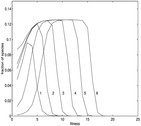
FIG. 1.: For $1\leq n\leq 6$ the $n$’th plot in the figure depicts the fitness distribution $P(x,t)$ at time $t=10^{n}$ The parameters used are $\alpha=1$, $b=1$ and $g=40$.

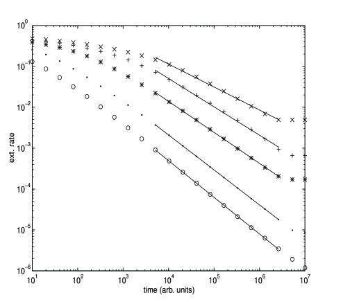
FIG. 2.: The numerically obtained extinction rate is plotted vs time, for $b=1$, $\alpha=0.95$ and for $g=5$ ($o$), $10$ (.), $20$ ($*$), $30$ ($+$) and $40$ ($\times$). The decay is approximately a power-law with exponents equal to $-0.89,-0.85,-0.75,-0.69$ and $-0.56$. These slopes are visualized by the full lines.

REFERENCES

- [1] On leave of absence from: Fysisk Institut, Odense Universitet, Campusvej 55, DK5230 Odense M, Denmark.
- [2] Paolo Sibani, Michel R. Schmidt and Preben Alstrøm Phys. Rev. Lett., 75, 2055 (1995)
- [3] P. Bak and K. Sneppen Phys. Rev. Lett., 71, 4083 (1993)
- [4] Kim Sneppen, Per Bak, Henrik Flyvbjerg and Mogens H. Jensen. Proc. Natl. Acad. Sci. USA, 92, 5209 (1995)
- [5] M. E. J. Newman and B. W. Roberts Proc. R. Soc. Lond. B , 260, 31, (1995)
- [6] S. Wright Evolution, 36, 427 (1982)
- [7] David M. Raup Paleobiology, 4, 42 (1978)
- [8] David M. Raup, The role of extinction in evolution, in Tempo and mode in evolution, edited by Walter M. Fitch and Francisco J. Ayala, National Academy of Sciences, (1995), pp. 109-124.
- [9] David M. Raup and J. John Sepkoski Science, 215, 1501 (1982)
- [10] Stephen Jay Gould Full House The spread of excellence from Plato to Darwin, Harmony Books, New York (1996)
- [11] Richard E. Lenski and Michael Travisano, Dynamics of adaptation and diversification, in Tempo and mode in evolution, sdited by Walter M. Fitch and Francisco J. Ayala, National Academy of Sciences, (1995), pp. 253-273.
- [12] Stuart Kauffman At home in the universe, Oxford University Press, p. 194, (1995)
- [13] Steven M. Stanley Paleobiology, 4, 26 (1978)
- [14] David M. Raup Paleobiology, 11, 42 (1985)
- [15] David M. Raup Science, 231, 1528(1986)
- [16] Tomasz K. Baumiller Paleobiology, 19, 304 (1993)
- [17] Paolo Sibani and Peter B. Littlewood Phys. Rev. Lett., 71, 1485 (1993)
- [18] S. A. Kauffman and S. Levin J. Theor. Biol., 128, 11 (1987)
- [19] J. J. Sepkoski Paleobiology 19, 43 (1993)
- [20] The ’birth and death’ formula [21] depends exponentially on the number of species initially in the genus. In the application one needs . It is also appreciated that this model cannot account for the appearance of new genera, as the parameter choice used to fit the data would otherwise imply the total extinction of life[7, 16].
- [21] Norman T. J. Bailey The elements of stochastic processes, John Wiley & Sons, (1964) pp. 93-94
- [22] Michael Brandt Stochastic evolution models . Master Thesis, Physics Dept. Odense University, January 1997.
- [23] S. C. Manrubia and M. Paczuski cond-mat preprint 9607066