Analytic Continuation of Bernoulli Numbers,

a New Formula for the Riemann Zeta Function,

and the Phenomenon of Scattering of Zeros 111Preprint DAMTP-R-97/19 on-line at http://www.damtp.cam.ac.uk/user/scw21/papers/


S.C. Woon

Department of Applied Mathematics and Theoretical Physics

University of Cambridge, Silver Street, Cambridge CB3 9EW, UK

Email: S.C.Woon@damtp.cam.ac.uk

Abstract

The method analytic continuation of operators acting integer $n$-times to complex s๐‘ s-times (hep-th/9707206) is applied to an operator that generates Bernoulli numbers $B_{n}$ (Math. Mag., 70(1), 51 (1997)). $B_{n}$ and Bernoulli polynomials Bnโ€‹(s)subscript๐ต๐‘›๐‘ B_{n}(s) are analytic continued to Bโ€‹(s)๐ต๐‘ B(s) and Bsโ€‹(z)subscript๐ต๐‘ ๐‘งB_{s}(z). A new formula for the Riemann zeta function ฮถโ€‹(s)๐œ๐‘ \zeta(s) in terms of nested series of $\zeta(n)$ is derived. The new concept of dynamics of the zeros of analytic continued polynomials is introduced, and an interesting phenonmenon of โ€˜scatteringsโ€™ of the zeros of Bsโ€‹(z)subscript๐ต๐‘ ๐‘งB_{s}(z) is observed.

1 Introduction: Bernoulli Numbers

Bernoulli numbers $B_{n}$ were discovered by Jakob Bernoulli (1654-1705) [1]. They are defined [2] [3] as

$$\frac{z}{e^{z}-1}\,=\,\sum_{n=0}^{\infty}\frac{B_{n}}{n!}z^{n}\;,\quad|z|<2\pi\;,\;\;n=1,2,3,\dots\in\mbox{\mbox{\sf Z}}^{+}$$ (1)

Expanding the l.h.s. as a series and matching the coefficients on both sides gives

B1=โˆ’1/2,Bnโ€‹{=0,oddย โ€‹nโ‰ 0,evenย โ€‹nsubscript๐ต112subscript๐ต๐‘›casesabsent0absentoddย ๐‘›absent0absentevenย ๐‘›B_{1}=-1/2,\quad B_{n}\left\{\begin{array}[]{ccc}=0&,&\mbox{odd }n\\ \neq 0&,&\mbox{even }n\end{array}\right. (2)

With this result, (1) can be rewritten as

$$\frac{z}{e^{z}-1}+\frac{z}{2}\,=\,\sum_{n=0}^{\infty}\frac{B_{2n}}{2n!}z^{2n}$$ (3)

Alternatively, Bernoulli numbers can be defined as satisfying the recurrence relation

$$B_{n}\,=\,-\,\frac{1}{n+1}\,\sum_{k=0}^{n-1}\,{n+1\choose k}\,B_{k}\;,\quad B_{0}=1$$ (4)

Bernoulli numbers are interesting numbers. They appear in connection with a wide variety of areas, from Euler-Maclaurin Summation formula in Analysis [4] [5] and the Riemann zeta function in Number Theory [6] [7], to Kummerโ€™s regular primes in special cases of Fermatโ€™s Last Theorem and Combinatorics [8].

2 A Tree for Generating Bernoulli Numbers

It was shown in [4] how a binary Tree for generating Bernoulli numbers can be intuited step-by-step and eventually discovered. In the process of calculating the analytic continuation of the Riemann zeta function to the negative half plane term-by-term, an emerging pattern was observed. The big picture of the structure of the Tree became apparent on comparing the derived expressions with the Euler-Maclaurin Summation formula.

In this paper, we start with the Tree and proceed on to find interesting applications. While doing so, we will encounter some surprising consequences.

The Tree can be constructed using two operators, $O_{L}$ and $O_{R}$.

At each node of the Tree sits a formal expression of the form $\displaystyle\frac{\pm 1}{a!\,b!\dots}$.

Define $O_{L}$ and $O_{R}$ to act only on formal expressions of this form at the nodes of the Tree as follows:

$\displaystyle O_{L}$ $\displaystyle:$ $\displaystyle\frac{\pm 1}{a!\,b!\dots}\to\frac{\mp 1}{(a+1)!\,b!\dots}$ (5)
$\displaystyle O_{R}$ $\displaystyle:$ $\displaystyle\frac{\pm 1}{a!\,b!\dots}\to\frac{\pm 1}{2!\,a!\,b!\dots}$ (6)

Schematically,

  • โ€ข

    OLsubscript๐‘‚๐ฟO_{L} acting on a node of the Tree generates a branch downwards to the left (hence the subscript L in $O_{L}$) with a new node at the end of the branch.

  • โ€ข

    ORsubscript๐‘‚๐‘…O_{R} acting on the same node generates a branch downwards to the right.

Refer to caption
Figure 1: The binary Tree that generates Bernoulli numbers.

Form a finite series out of the sum of the two non-commuting operators

$$S_{n}\,=\,(O_{L}+O_{R})^{n}\left(\frac{+1}{2!}\right)\,=\,\left(O_{L}^{n}+\sum_{k=0}^{n-1}O_{L}^{n-1-k}O_{R}O_{L}^{k}+\cdots+O_{R}^{n}\right)\left(\frac{+1}{2!}\right)$$ (7)

This is equivalent to summing terms on the $n$-th row of nodes across the Tree.

Bernoulli numbers are then simply given by

$$B_{n}\,=\,n!\;S_{n-1}\quad\mbox{for }\;n\geq 2$$ (8)
$$\mbox{eg., }B_{3}\,=\,3!\;S_{2}\,=\,3!\;(O_{L}+O_{R})^{2}\left(\frac{+1}{2!}\right)\,=\,3!\;(O_{L}+O_{R})\,(O_{L}+O_{R})\left(\frac{+1}{2!}\right)$$
$$=\,3!\;(O_{L}O_{L}+O_{L}O_{R}+O_{R}O_{L}+O_{R}O_{R})\left(\frac{+1}{2!}\right)$$
$$=\,3!\;\left(\frac{+1}{4!}+\frac{-1}{2!3!}+\frac{-1}{3!2!}+\frac{+1}{2!2!2!}\right)=0$$

By observation, this Sum-across-the-Tree representation of $\,S_{n}\,$ is exactly equivalent to the following determinant known to generate $B_{n}$,

$$S_{n}=(-1)^{n}\left|\begin{array}[]{ccccccc}\displaystyle\Bigg{.}\frac{1}{2!}&1&0&\;\quad 0&\;\quad 0&\;\cdots&\;\;\;0\\ \displaystyle\Bigg{.}\frac{1}{3!}&\displaystyle\frac{1}{2!}&1&0&0&\cdots&\;\;\;0\\ \displaystyle\Bigg{.}\frac{1}{4!}&\displaystyle\frac{1}{3!}&\displaystyle\frac{1}{2!}&1&0&\cdots&\;\;\;0\\ \displaystyle\Bigg{.}\vdots&\ddots&\ddots&\ddots&\ddots&\ddots&\;\;\;\vdots\\ \displaystyle\Bigg{.}\frac{1}{(n-2)!}&\ddots&\ddots&\displaystyle\frac{1}{3!}&\displaystyle\frac{1}{2!}&1&\;\;\;0\\ \displaystyle\Bigg{.}\frac{1}{(n-1)!}&\displaystyle\frac{1}{(n-2)!}&\ddots&\ddots&\displaystyle\frac{1}{3!}&\displaystyle\frac{1}{2!}&\;\;\;1\\ \displaystyle\Bigg{.}\frac{1}{n!}&\displaystyle\frac{1}{(n-1)!}&\displaystyle\frac{1}{(n-2)!}&\ddots&\ddots&\displaystyle\frac{1}{3!}&\;\;\;\displaystyle\frac{1}{2!}\end{array}\right|$$ (9)

3 Analytic Continuations

3.1 Analytic Continuation of Operator

First, we introduce the idea of analytic continuing the action of an operator following [9]. We are used to thinking of an operator acting once, twice, three times, and so on. However, an operator acting integer times can be analytic continued to an operator acting complex times by making the following observation:

A generic operator $A$ acting complex s๐‘ s-times can be formally expanded into a series as

Assuperscript๐ด๐‘ \displaystyle A^{s} $\displaystyle=$ $\displaystyle\left(\Big{.}w\mbox{\bf 1}-\left[\big{.}w\mbox{\bf 1}-A\right]\right)^{\!s}=w^{s}\Big{(}1-\Big{[}1-\frac{1}{w}A\Big{]}\Big{)}^{\!s}$ (10)
$\displaystyle=$ $\displaystyle w^{s}\!\left(\mbox{\bf 1}+\sum_{n=1}^{\infty}\frac{(-1)^{n}}{n!}\left[\prod_{k=0}^{n-1}(s\!-\!k)\right]\!\left[\big{.}\mbox{\bf 1}-\frac{1}{w}A\right]^{\!n}\right)$
$\displaystyle=$ wsโ€‹(1+โˆ‘n=1โˆž(โˆ’1)nn!โ€‹[โˆk=0nโˆ’1(sโˆ’k)]โ€‹[1+โˆ‘m=1n(โˆ’1w)mโ€‹(nm)โ€‹Am])superscript๐‘ค๐‘ 1superscriptsubscript๐‘›1superscript1๐‘›๐‘›delimited-[]superscriptsubscriptproduct๐‘˜0๐‘›1๐‘ ๐‘˜delimited-[]1superscriptsubscript๐‘š1๐‘›superscript1๐‘ค๐‘šbinomial๐‘›๐‘šsuperscript๐ด๐‘š\displaystyle w^{s}\!\left(\mbox{\bf 1}+\sum_{n=1}^{\infty}\frac{(-1)^{n}}{n!}\left[\prod_{k=0}^{n-1}(s\!-\!k)\right]\!\left[\mbox{\bf 1}+\sum_{m=1}^{n}\left(\frac{-1}{w}\right)^{\!\!m}\!\!{n\choose m}A^{m}\right]\right)

where sโˆˆC๐‘ C\;s\in\mbox{\sf C}, $w\in\mbox{\sf R}$, and โ€…1โ€… is the identity operator.

The region of convergence in s๐‘ \,s\, and the rate of convergence of the series will in general be dependent on operator $A,\;$ parameter $w,\;$ and the operand on which $A$ acts.

3.2 Analytic Continuation of the Tree-Generating Operator

Just as in (10), the Tree-generating operator $(O_{L}+O_{R})$ acting (sโˆ’1)๐‘ 1(s-1) times on $\displaystyle\left(\frac{+1}{2!}\right)$ can be similarly expanded as

(OL+OR)sโˆ’1โ€‹(+12!)superscriptsubscript๐‘‚๐ฟsubscript๐‘‚๐‘…๐‘ 112\displaystyle(O_{L}+O_{R})^{s-1}\left(\frac{+1}{2!}\right)
$\displaystyle=$ wsโ€‹(1+โˆ‘n=1โˆž(โˆ’1)nn!โ€‹[โˆk=1n(sโˆ’k)]โ€‹[1+โˆ‘m=1n(โˆ’1w)mโ€‹(nm)โ€‹(OL+OR)m])โ€‹(+12!)superscript๐‘ค๐‘ 1superscriptsubscript๐‘›1superscript1๐‘›๐‘›delimited-[]superscriptsubscriptproduct๐‘˜1๐‘›๐‘ ๐‘˜delimited-[]1superscriptsubscript๐‘š1๐‘›superscript1๐‘ค๐‘šbinomial๐‘›๐‘šsuperscriptsubscript๐‘‚๐ฟsubscript๐‘‚๐‘…๐‘š12\displaystyle w^{s}\left(\mbox{\bf 1}+\sum_{n=1}^{\infty}\frac{(-1)^{n}}{n!}\left[\prod_{k=1}^{n}(s\!-\!k)\right]\!\left[\mbox{\bf 1}+\sum_{m=1}^{n}\left(\frac{-1}{w}\right)^{\!\!m}\!\!{n\choose m}(O_{L}+O_{R})^{m}\right]\right)\!\left(\frac{+1}{2!}\right)
$\displaystyle=$ wsโ€‹(12+โˆ‘n=1โˆž(โˆ’1)nn!โ€‹[โˆk=1n(sโˆ’k)]โ€‹[12+โˆ‘m=1n(โˆ’1w)mโ€‹(nm)โ€‹Bm+1(m+1)!])superscript๐‘ค๐‘ 12superscriptsubscript๐‘›1superscript1๐‘›๐‘›delimited-[]superscriptsubscriptproduct๐‘˜1๐‘›๐‘ ๐‘˜delimited-[]12superscriptsubscript๐‘š1๐‘›superscript1๐‘ค๐‘šbinomial๐‘›๐‘šsubscript๐ต๐‘š1๐‘š1\displaystyle w^{s}\left(\frac{1}{2}+\sum_{n=1}^{\infty}\frac{(-1)^{n}}{n!}\left[\prod_{k=1}^{n}(s\!-\!k)\right]\!\left[\frac{1}{2}+\sum_{m=1}^{n}\left(\frac{-1}{w}\right)^{\!\!m}\!\!{n\choose m}\frac{B_{m+1}}{(m\!+\!1)!}\right]\right) (11)

which converges for Re(s)>(1/w)๐‘ 1๐‘ค(s)>(1/w)\; where sโˆˆC๐‘ C\;s\in\mbox{\sf C}, $\;w\in\mbox{\sf R}$, $\;w>0$.

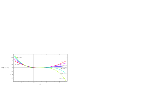
3.3 Analytic Continuation of Bernoulli Numbers

$$B_{n}\,=\,n!\;(O_{L}+O_{R})^{n-1}\left(\frac{+1}{2!}\right)\,=\,\Gamma(1+n)\;(O_{L}+O_{R})^{n-1}\left(\frac{+1}{2!}\right)$$

Now that we can analytic continue the Tree-generating operator $(O_{L}+O_{R})$ with (11), if we do so, we turn the sequence of Bernoulli numbers $B_{n}$ into their analytic continuation โ€” a function

Bโ€‹(s)=ฮ“โ€‹(1+s)โ€‹(OL+OR)sโˆ’1โ€‹(+12!)๐ต๐‘ ฮ“1๐‘ superscriptsubscript๐‘‚๐ฟsubscript๐‘‚๐‘…๐‘ 112\displaystyle B(s)\;=\;\Gamma(1+s)\;(O_{L}+O_{R})^{s-1}\left(\frac{+1}{2!}\right) (12)
$\displaystyle=$ wsโ€‹ฮ“โ€‹(1+s)โ€‹(12+โˆ‘n=1โˆž(โˆ’1)nn!โ€‹[โˆk=1n(sโˆ’k)]โ€‹[12+โˆ‘m=1n(โˆ’1w)mโ€‹(nm)โ€‹Bm+1(m+1)!])superscript๐‘ค๐‘ ฮ“1๐‘ 12superscriptsubscript๐‘›1superscript1๐‘›๐‘›delimited-[]superscriptsubscriptproduct๐‘˜1๐‘›๐‘ ๐‘˜delimited-[]12superscriptsubscript๐‘š1๐‘›superscript1๐‘ค๐‘šbinomial๐‘›๐‘šsubscript๐ต๐‘š1๐‘š1\displaystyle w^{s}\;\Gamma(1+s)\left(\frac{1}{2}+\sum_{n=1}^{\infty}\frac{(-1)^{n}}{n!}\left[\prod_{k=1}^{n}(s\!-\!k)\right]\!\left[\frac{1}{2}+\sum_{m=1}^{n}\left(\frac{-1}{w}\right)^{\!\!m}\!\!{n\choose m}\frac{B_{m+1}}{(m\!+\!1)!}\right]\right)

which converges for โ€…Re(s)>(1/w),๐‘ 1๐‘ค(s)>(1/w)\;,\; real $\;w>0.$

So effectively, by the method of analytic continuation of operator, we have now obtained the function Bโ€‹(s)๐ต๐‘ \;B(s)\; as the analytic continuation of Bernoulli numbers.

Refer to caption
Figure 2: The curve Bโ€‹(s)๐ต๐‘ \,B(s)\, runs through the points of all $\,B_{n}$ except $\,B_{1}$.

All the Bernoulli numbers $B_{n}$ agree with $B(n)$, the analytic continuation of Bernoulli numbers evaluated at $n$,

$$B(n)\,=\,B_{n}\quad\mbox{for}\quad n\geq 2$$ (13)
$$\mbox{except}\quad\quad B(1)=\frac{1}{2}\quad\mbox{ but }\quad B_{1}=-\,\frac{1}{2}\quad\quad\quad\quad$$ (14)

4 Missing Signs in the Definition of $B_{n}$

Looking back at (1) to (4), we can see that the sign convention of $B_{1}$ was actually arbitrary. (14) suggests that consistent definition of Bernoulli numbers should really have been

$$\frac{z}{e^{z}-1}\,=\,\sum_{n=0}^{\infty}(-1)^{n}\frac{B_{n}}{n!}z^{n}\;,\quad|z|<2\pi\;,\;\;n=1,2,3,\dots\in\mbox{\mbox{\sf Z}}^{+}$$ (15)

or

$$B_{n}\,=\,\frac{(-1)^{n+1}}{n+1}\,\sum_{k=0}^{n-1}\,(-1)^{k}\,{n+1\choose k}\,B_{k}\;,\quad B_{0}=1$$ (16)

which only changes the sign in the conventional definition of the only non-zero odd Bernoulli numbers, $B_{1}$, from $\;B_{1}=-1/2\;$ to $\;B_{1}=B(1)=1/2\;$.

So hereโ€™s my little appeal to the Mathematics, Physics, Engineering, and Computing communities to introduce the missing signs into the sum in the definition of Bernoulli numbers as in (15) and (16) because the analytic continuation of Bernoulli numbers fixes the arbitrariness of the sign convention of $B_{1}$.

5 A New Formula for the Riemann Zeta Function

Bernoulli numbers are related to the Riemann zeta function as [2] [3]

$$\zeta(-n)\,=\,-\;\frac{B_{n+1}}{n+1}$$ (17)
$$\zeta(2n)\,=\,\frac{(-1)^{n+1}(2\pi)^{2n}}{2\;(2n)!}B_{2n}$$ (18)

for $\;n=0,1,2,\dots\in$ Z${}^{+}_{0}$.

From the above analytic continuation of Bernoulli numbers,

$\displaystyle B_{n}$ $\displaystyle\mapsto$ Bโ€‹(s)๐ต๐‘ \displaystyle B(s)
$\displaystyle\left(\zeta(-n)\,=\,-\;\frac{B_{n+1}}{n+1}\right)$ $\displaystyle\mapsto$ (ฮถโ€‹(โˆ’s)=โˆ’Bโ€‹(s+1)s+1)๐œ๐‘ ๐ต๐‘ 1๐‘ 1\displaystyle\left(\zeta(-s)\,=\,-\;\frac{B(s+1)}{s+1}\right)
โ‡’ฮถโ€‹(1โˆ’s)โ‡’๐œ1๐‘ \displaystyle\Rightarrow\quad\zeta(1-s) $\displaystyle=$ โˆ’Bโ€‹(s)s๐ต๐‘ ๐‘ \displaystyle-\;\frac{B(s)}{s} (19)

Replacing Bโ€‹(s)๐ต๐‘ B(s) in (19) with the series in (12) and noting that ฮ“โ€‹(1+s)/s=ฮ“โ€‹(s)ฮ“1๐‘ ๐‘ ฮ“๐‘ \;\Gamma(1+s)/s=\Gamma(s)\; gives

ฮถโ€‹(1โˆ’s)=โˆ’wsโ€‹ฮ“โ€‹(s)โ€‹(12+โˆ‘n=1โˆž(โˆ’1)nn!โ€‹[โˆk=1n(sโˆ’k)]โ€‹[12+โˆ‘m=1n(โˆ’1w)mโ€‹(nm)โ€‹Bm+1(m+1)!])๐œ1๐‘ superscript๐‘ค๐‘ ฮ“๐‘ 12superscriptsubscript๐‘›1superscript1๐‘›๐‘›delimited-[]superscriptsubscriptproduct๐‘˜1๐‘›๐‘ ๐‘˜delimited-[]12superscriptsubscript๐‘š1๐‘›superscript1๐‘ค๐‘šbinomial๐‘›๐‘šsubscript๐ต๐‘š1๐‘š1\zeta(1-s)=-\;w^{s}\;\Gamma(s)\left(\frac{1}{2}+\sum_{n=1}^{\infty}\frac{(-1)^{n}}{n!}\left[\prod_{k=1}^{n}(s\!-\!k)\right]\!\left[\frac{1}{2}+\sum_{m=1}^{n}\left(\frac{-1}{w}\right)^{\!\!m}\!\!{n\choose m}\frac{B_{m+1}}{(m+1)!}\right]\right) (20)

which converges for Re(1โˆ’s)<1โˆ’(1/w),1๐‘ 11๐‘ค(1-s)<1-(1/w)\;,\; real $\;w>0$.

The functional equation of the Riemann zeta function relates ฮถโ€‹(1โˆ’s)๐œ1๐‘ \zeta(1-s) to ฮถโ€‹(s)๐œ๐‘ \zeta(s) as

ฮถโ€‹(1โˆ’s)=2โ€‹(2โ€‹ฯ€)โˆ’sโ€‹ฮ“โ€‹(s)โ€‹cosโก(ฯ€โ€‹s2)โ€‹ฮถโ€‹(s)๐œ1๐‘ 2superscript2๐œ‹๐‘ ฮ“๐‘ ๐œ‹๐‘ 2๐œ๐‘ \zeta(1-s)=2\;(2\pi)^{-s}\;\Gamma(s)\;\cos\left(\frac{\pi s}{2}\right)\;\zeta(s) (21)

Applying this relation to (20) yields

cosโก(ฯ€โ€‹s^2)โ€‹ฮถโ€‹(s)=โˆ’(2โ€‹ฯ€โ€‹w)s2โ€‹(12+โˆ‘n=1โˆž(โˆ’1)nn!โ€‹[โˆk=1n(sโˆ’k)]โ€‹[12+โˆ‘m=1n(โˆ’1w)mโ€‹(nm)โ€‹Bm+1(m+1)!])๐œ‹^๐‘ 2๐œ๐‘ superscript2๐œ‹๐‘ค๐‘ 212superscriptsubscript๐‘›1superscript1๐‘›๐‘›delimited-[]superscriptsubscriptproduct๐‘˜1๐‘›๐‘ ๐‘˜delimited-[]12superscriptsubscript๐‘š1๐‘›superscript1๐‘ค๐‘šbinomial๐‘›๐‘šsubscript๐ต๐‘š1๐‘š1\!\!\!\!\!\!\!\!\!\!\!\cos\left(\frac{\pi\hat{s}}{2}\right)\zeta(s)=-\;\frac{(2\pi w)^{s}}{2}\left(\frac{1}{2}+\sum_{n=1}^{\infty}\frac{(-1)^{n}}{n!}\left[\prod_{k=1}^{n}(s\!-\!k)\right]\!\left[\frac{1}{2}+\sum_{m=1}^{n}\left(\frac{-1}{w}\right)^{\!\!m}\!\!{n\choose m}\frac{B_{m+1}}{(m+1)!}\right]\right) (22)

or in the limiting form

ฮถโ€‹(s)=โˆ’(2โ€‹ฯ€โ€‹w)s2โ€‹lims^โ†’s{(12+โˆ‘n=1โˆž(โˆ’1)nn!โ€‹[โˆk=1n(s^โˆ’k)]โ€‹[12+โˆ‘m=1n(โˆ’1w)mโ€‹(nm)โ€‹Bm+1(m+1)!])cosโก(ฯ€โ€‹s^2)}๐œ๐‘ superscript2๐œ‹๐‘ค๐‘ 2subscriptโ†’^๐‘ ๐‘ 12superscriptsubscript๐‘›1superscript1๐‘›๐‘›delimited-[]superscriptsubscriptproduct๐‘˜1๐‘›^๐‘ ๐‘˜delimited-[]12superscriptsubscript๐‘š1๐‘›superscript1๐‘ค๐‘šbinomial๐‘›๐‘šsubscript๐ต๐‘š1๐‘š1๐œ‹^๐‘ 2\!\!\!\!\!\!\!\!\!\!\zeta(s)=-\;\frac{(2\pi w)^{s}}{2}\lim_{\;{\displaystyle\hat{s}}\to{\displaystyle s}}\left\{\!\frac{\left(\displaystyle\frac{1}{2}+\sum_{n=1}^{\infty}\frac{(-1)^{n}}{n!}\left[\prod_{k=1}^{n}(\hat{s}\!-\!k)\right]\left[\frac{1}{2}+\sum_{m=1}^{n}\left(\frac{-1}{w}\right)^{\!\!m}\!\!{n\choose m}\frac{B_{m+1}}{(m+1)!}\right]\!\right)}{\displaystyle\cos\left(\frac{\pi\hat{s}}{2}\right)}\right\}
=โˆ’(2โ€‹ฯ€โ€‹w)s2โ€‹lims^โ†’s{(12+โˆ‘n=1โˆž(โˆ’1)nn!โ€‹[โˆk=1n(s^โˆ’k)]โ€‹[12โˆ’โˆ‘m=1n(โˆ’1w)mโ€‹(nm)โ€‹ฮถโ€‹(โˆ’m)m!])cosโก(ฯ€โ€‹s^2)}absentsuperscript2๐œ‹๐‘ค๐‘ 2subscriptโ†’^๐‘ ๐‘ 12superscriptsubscript๐‘›1superscript1๐‘›๐‘›delimited-[]superscriptsubscriptproduct๐‘˜1๐‘›^๐‘ ๐‘˜delimited-[]12superscriptsubscript๐‘š1๐‘›superscript1๐‘ค๐‘šbinomial๐‘›๐‘š๐œ๐‘š๐‘š๐œ‹^๐‘ 2=-\;\frac{(2\pi w)^{s}}{2}\lim_{\;{\displaystyle\hat{s}}\to{\displaystyle s}}\left\{\!\frac{\left(\displaystyle\frac{1}{2}+\sum_{n=1}^{\infty}\frac{(-1)^{n}}{n!}\left[\prod_{k=1}^{n}(\hat{s}\!-\!k)\right]\left[\frac{1}{2}-\sum_{m=1}^{n}\left(\frac{-1}{w}\right)^{\!\!m}\!\!{n\choose m}\frac{\zeta(-m)}{m!}\right]\!\right)}{\displaystyle\cos\left(\frac{\pi\hat{s}}{2}\right)}\right\} (23)

a nested sum of the Riemann zeta function itself evaluated at negative integers, which converges for Re(s)>(1/w),๐‘ 1๐‘ค(s)>(1/w)\;,\; real $\;w>0\;,\;$ and the limit only needs to be taken when $\;s=1,3,5,\dots\in$ Z${}^{+}_{odd}$, the set of positive odd integers, for which the denominator cosโก(ฯ€โ€‹s2)=0๐œ‹๐‘ 20\;\displaystyle\cos\left(\frac{\pi s}{2}\right)=0.

This is consistent with

(ฮถโ€‹(2โ€‹n)=(โˆ’1)n+1โ€‹(2โ€‹ฯ€)2โ€‹n2โ€‹(2โ€‹n)!โ€‹B2โ€‹n)โ†ฆ(ฮถโ€‹(2โ€‹s)=โˆ’(2โ€‹ฯ€)2โ€‹s2โ€‹ฮ“โ€‹(1+2โ€‹s)โ€‹lims^โ†’s{Bโ€‹(2โ€‹s^)cosโก(ฯ€โ€‹s^)})maps-to๐œ2๐‘›superscript1๐‘›1superscript2๐œ‹2๐‘›22๐‘›subscript๐ต2๐‘›๐œ2๐‘ superscript2๐œ‹2๐‘ 2ฮ“12๐‘ subscriptโ†’^๐‘ ๐‘ ๐ต2^๐‘ ๐œ‹^๐‘ \left(\zeta(2n)\,=\,\frac{(-1)^{n+1}(2\pi)^{2n}}{2\;(2n)!}B_{2n}\right)\;\;\mapsto\;\;\left(\zeta(2s)\,=\,-\,\frac{(2\pi)^{2s}}{\displaystyle 2\;\Gamma(1+2s)}\,\lim_{\;{\displaystyle\hat{s}}\to{\displaystyle s}}\,\left\{\frac{B(2\hat{s})}{\cos(\pi\hat{s})}\right\}\right)
โ‡’ฮถโ€‹(s)=โˆ’(2โ€‹ฯ€)s2โ€‹ฮ“โ€‹(1+s)โ€‹lims^โ†’s{Bโ€‹(s^)cosโก(ฯ€โ€‹s^2)}โ‡’๐œ๐‘ superscript2๐œ‹๐‘ 2ฮ“1๐‘ subscriptโ†’^๐‘ ๐‘ ๐ต^๐‘ ๐œ‹^๐‘ 2\Rightarrow\quad\zeta(s)\;\;=\;\;-\,\frac{(2\pi)^{s}}{\displaystyle 2\;\Gamma(1+s)}\lim_{\;{\displaystyle\hat{s}}\to{\displaystyle s}}\,\left\{\frac{B(\hat{s})}{\cos\left(\displaystyle\frac{\pi\hat{s}}{2}\right)}\right\}\quad (24)
Refer to caption
Figure 3: Wโ€‹(s)=(2โ€‹ฯ€)sโ€‹Bโ€‹(s)2โ€‹ฮ“โ€‹(1+s)=โˆ’cosโก(ฯ€โ€‹s2)โ€‹ฮถโ€‹(s).Wโ€‹(s)formulae-sequence๐‘Š๐‘ superscript2๐œ‹๐‘ ๐ต๐‘ 2ฮ“1๐‘ ๐œ‹๐‘ 2๐œ๐‘ ๐‘Š๐‘ \displaystyle\;W(s)\,=\,\frac{(2\pi)^{s}\;B(s)}{2\;\Gamma(1+s)}=-\,\cos\left(\displaystyle\frac{\pi s}{2}\right)\,\zeta(s).\;\;W(s) is bounded by the envelopes $\Big{.}\,\pm\left|\zeta(s)\right|\;$ shown as dashed curves.

Since both $\,B(k)\,$ and $\,\cos\left(\displaystyle\frac{\pi k}{2}\right)=0\,$ for odd integer $\,k\in$ Z${}^{+}_{odd}\backslash\{1\}$, Lโ€™Hรถpital rule can be applied to the limit giving

lims^โ†’s{Bโ€‹(s^)cosโก(ฯ€โ€‹s^2)}={Bโ€‹(s)cosโก(ฯ€โ€‹s2),sโˆ‰Zoโ€‹dโ€‹d+โˆž,s=1(โˆ’1)(s+1)/2โ€‹2โ€‹Bโ€ฒโ€‹(s)ฯ€,sโˆˆZoโ€‹dโ€‹d+\{1}subscriptโ†’^๐‘ ๐‘ ๐ต^๐‘ ๐œ‹^๐‘ 2cases๐ต๐‘ ๐œ‹๐‘ 2absent๐‘ subscriptsuperscriptZ๐‘œ๐‘‘๐‘‘missing-subexpressionmissing-subexpressionmissing-subexpressionabsent๐‘ 1missing-subexpressionmissing-subexpressionmissing-subexpressionsuperscript1๐‘ 122superscript๐ตโ€ฒ๐‘ ๐œ‹absent๐‘ \subscriptsuperscriptZ๐‘œ๐‘‘๐‘‘1\lim_{{\displaystyle\hat{s}}\to{\displaystyle s}}\,\left\{\frac{B(\hat{s})}{\cos\left(\displaystyle\frac{\pi\hat{s}}{2}\right)}\right\}\,=\,\left\{\begin{array}[]{lcl}\displaystyle\frac{B(s)}{\cos\left(\displaystyle\frac{\pi s}{2}\right)}&,&s\not\in\mbox{\mbox{\sf Z}}^{+}_{odd}\\ &&\\ \infty&,&s=1\\ &&\\ \displaystyle(-1)^{(s+1)/2}\,\frac{2B^{\prime}(s)}{\pi}&,&s\in\mbox{\mbox{\sf Z}}^{+}_{odd}\backslash\{1\}\end{array}\right. (25)

where the prime denotes differentiation and so Bโ€ฒโ€‹(s)superscript๐ตโ€ฒ๐‘ \,B^{\prime}(s)\, is the derivative of the function Bโ€‹(s)๐ต๐‘ B(s).

Therefore we have now found the apparently missing โ€˜oddโ€™ expression โ€˜dualโ€™ to the โ€˜evenโ€™ expression (18).

$$\mbox{(even):}\quad\quad\quad\quad\quad\quad\quad\zeta(2n)\,=\,(-1)^{n+1}\displaystyle\frac{(2\pi)^{2n}}{(2n)!}\;\frac{B_{2n}}{2}\quad\quad\quad\quad\quad\quad\quad\quad\quad\quad\;$$ (26)
$$\mbox{(odd): }\quad\quad\quad\quad\quad\zeta(2n+1)\,=\,(-1)^{n}\displaystyle\frac{(2\pi)^{2n+1}}{(2n+1)!}\;\frac{B^{\prime}(2n+1)}{\pi}\quad\quad\quad\quad\quad\quad\quad$$ (27)

for $\;n=1,2,3,\dots\in$ Z+.

In fact, we can express Bโ€ฒโ€‹(s)superscript๐ตโ€ฒ๐‘ \,B^{\prime}(s)\, in terms of ฮถโ€ฒโ€‹(s)superscript๐œโ€ฒ๐‘ \,\zeta^{\prime}(s), the derivative of ฮถโ€‹(s)๐œ๐‘ \,\zeta(s).

Bโ€‹(s)๐ต๐‘ \displaystyle B(s) $\displaystyle=$ โˆ’sโ€‹ฮถโ€‹(1โˆ’s)๐‘ ๐œ1๐‘ \displaystyle-\;s\;\zeta(1-s)
Bโ€ฒโ€‹(s)superscript๐ตโ€ฒ๐‘ \displaystyle B^{\prime}(s) $\displaystyle=$ โˆ’ฮถโ€‹(1โˆ’s)+sโ€‹ฮถโ€ฒโ€‹(1โˆ’s)๐œ1๐‘ ๐‘ superscript๐œโ€ฒ1๐‘ \displaystyle-\;\zeta(1-s)\,+\,s\;\zeta^{\prime}(1-s)
$\displaystyle B^{\prime}(2n+1)$ $\displaystyle=$ $\displaystyle\quad(2n+1)\;\zeta^{\prime}(-2n)$
$\displaystyle\quad\quad\quad\mbox{as }\;\zeta(-2n)=0$
$$\quad\quad\quad\quad\quad\Rightarrow\quad\quad\zeta(2n+1)\,=\,(-1)^{n}\,\frac{(2\pi)^{2n+1}}{(2n)!\;\pi}\;\zeta^{\prime}(-2n)\;\quad\mbox{for }n\in\mbox{\mbox{\sf Z}}^{+}.$$ (29)

This is just the differential of the functional equation and so verifies the consistency of Bโ€‹(s)๐ต๐‘ B(s) and Bโ€ฒโ€‹(s)superscript๐ตโ€ฒ๐‘ B^{\prime}(s) with $B_{n}$ and ฮถโ€‹(s)๐œ๐‘ \zeta(s).

6 Other Undiscovered Half of Bernoulli Numbers

From the relation (19), we can define the other analytic continued half of Bernoulli Numbers

Bโ€‹(s)=โˆ’sโ€‹ฮถโ€‹(1โˆ’s),Bโ€‹(โˆ’s)=sโ€‹ฮถโ€‹(s+1)formulae-sequence๐ต๐‘ ๐‘ ๐œ1๐‘ ๐ต๐‘ ๐‘ ๐œ๐‘ 1B(s)\,=\,-\;s\;\zeta(1-s)\;,\quad B(-s)\,=\,s\;\zeta(s+1)
$$\Rightarrow\quad B_{-n}\,=\,B(-n)\,=\,n\;\zeta(n+1)\;,\quad n\in\mbox{\mbox{\sf Z}}^{+}$$ (30)

Since $\;\zeta(n+1)\to 1\;$ as $\;n\to\infty,\;\;B_{-n}\sim n\;$ asymptotically for $\;(-n)\ll-1$.

Refer to caption
Figure 4: The curve Bโ€‹(s)๐ต๐‘ \,B(s)\, runs through the points $\,B_{-n}$ and grows $\sim n\;$ asymptotically as $\,(-\,n)\,\to-\,\infty$.

7 More Related Analytic Continuations

7.1 Analytic Continuation of Bernoulli Polynomials

The conventional definition [2] [3] of Bernoulli polynomials $\,B_{n}(x)\,$ also has an arbitrariness in the sign convention. For consistency with the redefinition of $\,B_{n}\,=\,B(n)\,$ in (15) and (16), Bernoulli polynomials should be analogously redefined as

$$\frac{z\;e^{xz}}{e^{z}-1}\,=\,\left(\sum_{k=0}^{\infty}(-1)^{k}B_{k}\frac{z^{k}}{r!}\right)\!\!\left(\sum_{m=0}^{\infty}\frac{(x\,z)^{m}}{m!}\right)\,=\,\sum_{n=0}^{\infty}(-1)^{n}B_{n}(x)\frac{z^{n}}{n!}$$
$$\Rightarrow\quad B_{n}(x)\,=\,\sum_{k=0}^{n}\,(-1)^{(n+k)}\,{n\choose k}\,B_{k}\,x^{n-k}$$ (31)

The analytic continuation can be then obtained as

nโ†ฆsโˆˆR,sโ‰ฅ1,xโ†ฆwโˆˆCformulae-sequencemaps-to๐‘›๐‘ Rformulae-sequence๐‘ 1maps-to๐‘ฅ๐‘คCn\;\mapsto\;s\in\mbox{\sf R}\;,\;s\geq 1\;,\quad x\;\mapsto\;w\in\mbox{\sf C}
$$B_{k}\;\mapsto\;B\!\left(\big{.}k+(s\!-\![s])\right)\,=\,-\left(\big{.}k+(s\!-\![s])\right)\,\zeta\!\left(\big{.}1-(k+(s\!-\![s]))\right)$$
(nk)โ†ฆฮ“โ€‹(1+s)ฮ“โ€‹(1+k+(sโˆ’[s]))โ€‹ฮ“โ€‹(1+[s]โˆ’k)maps-tobinomial๐‘›๐‘˜ฮ“1๐‘ ฮ“1๐‘˜๐‘ delimited-[]๐‘ ฮ“1delimited-[]๐‘ ๐‘˜{n\choose k}\;\mapsto\;\frac{\Gamma(1+s)}{\Gamma(1+k+(s\!-\![s]))\;\Gamma(1+[s]-k)}
$$\Rightarrow\quad B_{n}(x)\;\mapsto\;B(s,w)\,=\,\sum_{k=-1}^{[s]}\frac{(1)^{n+k}\;\;\Gamma(1+s)\;\;B\!\left(\big{.}k+(s\!-\![s])\right)\;\;w^{[s]-k}}{\Gamma(1+k+(s\!-\![s]))\;\Gamma(1+[s]-k)}$$
$$\quad\quad\quad\quad\sum_{k=0}^{[s]+1}\frac{(1)^{n+k+1}\;\;\Gamma(1+s)\;\;B\!\left(\big{.}(k-1)+(s\!-\![s])\right)\;\;w^{[s]+1-k}}{\Gamma(k+(s\!-\![s]))\;\Gamma(2+[s]-k)}$$ (32)

where [s]delimited-[]๐‘ \;[s]\; gives the integer part of s,๐‘ \;s\,,\; and so (sโˆ’[s])๐‘ delimited-[]๐‘ \;(s\!-\![s])\; gives the fractional part,

$$\mbox{eg.,}\quad B_{2}(x)\,=\,B(2,x)\,=\,1/6-x+x^{2}\;\approx\,0.16667-x+x^{2}$$
$$B(2.01,x)\,\approx\,0.16420-0.99660\,x+1.00920\,x^{2}-0.00554\,x^{3}$$
$$B(2.99,x)\,\approx\,0.00092-0.50576\,x+1.50001\,x^{2}-0.98744\,x^{3}$$
$$B_{3}(x)\,=\,B(3,x)\,=\,-0.5\,x+1.5\,x^{2}-x^{3}$$
Refer to caption
Figure 5: Deformation of the curve of $\,B_{2}(x)\,=\,B(2,x)\,$ into the curve of $\,B_{3}(x)\,=\,B(3,x)\,$ via the real analytic continuation Bโ€‹(s,x),โ€„2โ‰คsโ‰ค3,xโˆˆR.formulae-sequence๐ต๐‘ ๐‘ฅ2๐‘ 3๐‘ฅR\,B(s,x),\;2\leq s\leq 3,\;x\in\mbox{\sf R}\,.

7.2 Analytic Continuation of Euler Numbers and Euler Polynomials

Euler numbers $\,E_{n}\,$ and Euler polynomials $\,E_{n}(x)\,$ are defined [2] [3] as

$$\mbox{sech }z\,=\,\frac{2\;e^{z}}{e^{2z+1}}\,=\,\sum_{n=0}^{\infty}E_{n}\frac{z^{n}}{n!}\,,\quad|z|<2\pi\,,\;n\in\mbox{\mbox{\sf Z}}^{+}\;;\;\;\;E_{n}=0\;\;\mbox{for odd}\;n$$ (33)
$$\frac{2\;e^{xz}}{e^{2z+1}}\,=\,\frac{2\;e^{z/2}\;e^{z(x-1/2)}}{(e^{z}+1)^{-1}}\,=\,\left(\sum_{k=0}^{\infty}E_{k}\frac{z^{k}}{2^{k}\,k!}\right)\!\!\left(\sum_{m=0}^{\infty}\frac{(x-\frac{1}{2}\Bigg{.})^{m}z^{m}}{m!}\right)\,=\,\sum_{n=0}^{\infty}E_{n}(x)\frac{z^{n}}{n!}$$
$$\Rightarrow\quad E_{n}(x)\,=\,\sum_{k=0}^{n}{n\choose r}\,2^{-r}\,(x-\frac{1}{2})^{n-r}\,E_{r}$$ (34)

and are related to Bernoulli polynomials as

$$E_{n}(x)\,=\,\frac{2}{n+1}\left(B_{n+1}(x)-2^{n+1}B_{n+1}\!\left(\frac{x}{2}\right)\right)$$ (35)
$$E_{n}\,=\,2^{n}E_{n}\!\left(\frac{1}{2}\right)\,=\,\frac{2}{n+1}\left(B_{n+1}\!\left(\frac{1}{2}\right)-2^{n+1}B_{n+1}\!\left(\frac{1}{4}\right)\right)$$ (36)

Their analytic continuation then follows straightforwardly from the analytic continuation of Bernoulli polynomials

Bnโ€‹(x)โ†ฆBโ€‹(s,w),Enโ†ฆEโ€‹(s),Enโ€‹(x)โ†ฆEโ€‹(s,w)formulae-sequencemaps-tosubscript๐ต๐‘›๐‘ฅ๐ต๐‘ ๐‘คformulae-sequencemaps-tosubscript๐ธ๐‘›๐ธ๐‘ maps-tosubscript๐ธ๐‘›๐‘ฅ๐ธ๐‘ ๐‘คB_{n}(x)\mapsto B(s,w)\,,\quad E_{n}\mapsto E(s)\,,\quad E_{n}(x)\mapsto E(s,w)

where nโ†ฆsโˆˆR,sโ‰ฅ1,xโ†ฆwโˆˆC.formulae-sequencemaps-to๐‘›๐‘ Rformulae-sequence๐‘ 1maps-to๐‘ฅ๐‘คC\;n\mapsto s\in\mbox{\sf R}\;,\;s\geq 1\;,\quad x\mapsto w\in\mbox{\sf C}\,.\quad

8 Beautiful zeros of Bernoulli Polynomials

8.1 Distribution and Structure of the zeros

Zeros of Bernoulli polynomials are solutions of $\,B_{n}(w)=0,\;w\in$ C.

Refer to caption
Figure 6: Zeros of Bernoulli polynomials $B_{80}(w)$.
Refer to caption
Figure 7: Stacks of zeros of Bernoulli polynomials $B_{n}(w)$ form a 3-D structure.

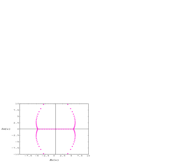
The real zeros, except the outermost pair in general, are almost regularly spaced, while the complex zeros lie on arcs symmetrical about Re$(w)=1/2$.

8.2 Observations, Theorem, Conjectures, and
Open Problems

  1. 1.

    Symmetries

    Prove that $\,B_{n}(w),\;w\in\,\mbox{\sf C},\,$ has $\,\mbox{\sf Re}(w)=1/2\,$ reflection symmetry in addition to the usual $\,\mbox{\sf Im}(w)=0\,$ reflection symmetry analytic complex functions. The obvious corollary is that the zeros of $\,B_{n}(w)\,$ will also inherit these symmetries.

    Ifย โ€‹Bnโ€‹(w0)=0,ย thenย โ€‹Bnโ€‹(1โˆ’w0)=0=Bnโ€‹(w0โ€ )=Bnโ€‹(1โˆ’w0โ€ )formulae-sequenceIfย subscript๐ต๐‘›subscript๐‘ค00ย thenย subscript๐ต๐‘›1subscript๐‘ค00subscript๐ต๐‘›superscriptsubscript๐‘ค0โ€ subscript๐ต๐‘›1superscriptsubscript๐‘ค0โ€ \mbox{If }\,B_{n}(w_{0})=0,\mbox{ then }\,B_{n}(1-w_{0})=0=B_{n}(w_{0}^{\dagger})=B_{n}(1-w_{0}^{\dagger}) (37)

    where โ€  denotes complex conjugation.


  2. 2.

    Non-degenerate zeros

    Prove that $\,B_{n}(w)=0\,$ has $\,n\,$ distinct solutions, ie., all the zeros are non-degenerate.


  3. 3.

    Central zero Theorem

    If $B_{2m+1}$ has $\,\mbox{\sf Re}(w)=1/2\,$ and $\,\mbox{\sf Im}(w)=0\,$ reflection symmetries, and $(2m+1)$ non-degenerate zeros, then $(2m)$ of the distinct zeros will satisfy (37). If the remaining one zero is to satisfy (37) too, it must reflect into itself, and therefore it must lie at 1/2, the center of the structure of the zeros, ie.,

    $$B_{n}(1/2)=0\quad\forall\;\mbox{ odd }\;n$$ (38)
  4. 4.

    Counting of real and complex zeros

    Prove that the number of complex zeros z${}_{\mbox{\scriptsize\sf C}(n)}$ of $\,B_{n}(w)\,$ lying on the 4 sets of arcs off the real plane, โ€†Im(w)โ‰ 0,๐‘ค0(w)\neq 0,\, is

    $$\mbox{\bf z}{}_{\mbox{\scriptsize\sf C}(n)}=4\left[\frac{n-\delta}{5}\right]\,,\mbox{ where }\;\delta=\left[\frac{n+30}{21}\right]$$ (39)

    and $\left[\big{.}\;\;\right]$ denotes taking the integer part. The factor 4 comes from the above 2 reflection symmetries.

    Since $\,n\,$ is the degree of the polynomial $\,B_{n}(w),\,$ the number of real zeros z${}_{\mbox{\scriptsize\sf R}(n)}$ lying on the real plane Im$(w)=0\,$ is then โ€… z${}_{\mbox{\scriptsize\sf R}(n)}=(n-$z${}_{\mbox{\scriptsize\sf C}(n)})$.

    See Appendix for tabulated values of z${}_{\mbox{\scriptsize\sf R}(n)}$ and z${}_{\mbox{\scriptsize\sf C}(n)}$.


  5. 5.

    Asymptotic Lattice of real zeros

    It is known that from (7.1),

    $$\sum_{n=0}^{\infty}\left(B_{n}(w+1)-B_{n}(w)\right)\frac{z^{n}}{n!}\,=\,z\,e^{wz}\,=\,\sum_{n=1}^{\infty}\frac{w^{n-1}\,z^{n}}{(n-1)!}$$
    $$\Rightarrow\quad B_{n}(w+1)-B_{n}(w)\,=\,w^{n-1}\quad\quad\quad\quad\quad\,$$
    $$\Rightarrow\quad B_{n}(1)=B_{n}(0)=B_{n}=0\quad\forall\;\mbox{ odd }\,n\geq 3$$

    Show that all the real zeros of $\,B_{n}(w)\,$ except the outermost pair in general, are approximately regularly spaced at the staggered lattice points

    $$w=\left\{\begin{array}[]{lll}\Big{.}0,\;\pm 1/2,\;\pm 1,\;\pm 3/2,\dots&\in\mbox{\mbox{\sf Z}}/2&\mbox{ for odd }\,n\\ \Big{.}\pm 1/4,\;\pm 3/4,\;\pm 5/4,\dots&\in\mbox{\mbox{\sf Z}}/2+1/4&\mbox{ for even }\,n\end{array}\right.$$ (40)

    and becomes increasingly located exactly at these lattice points as $\,n\to\infty$.

    Refer to captionRefer to caption\begin{array}[]{c}\psfig{height=170.0pt}\end{array}

    Figure 8: Inner real zeros converge to a staggered Lattice structure.

    See Appendix for tabulated solutions of $\,B_{n}(w)=0\,.$


  6. 6.

    Relation between zeros of Bernoulli and Euler polynomials

    Choose any zero of Bernoulli polynomial $\,B_{n}(w)\,$ and denote it as $\,w_{B(n)}$,
    ie. $\,B_{n}(w_{B(n)})=0$.

    Prove that

    $$\mbox{as }\;n\to\infty\,,\;\;\;E_{n}\!\left(2\;(w_{B(n)}-1/2)+1/2\right)=E_{n}\!\left(2\;w_{B(n)}-1/2\right)=0$$ (41)

    ie., the structure of the zeros of Euler polynomials resembles the structure of the zeros of Bernoulli polynomials but doubled in size in the limit the degree of the polynomials $\,n\to\infty$. Both structures are centered at $\,w=1/2$.


  7. 7.

    Bounding Envelopes and Trajectories of complex zeros

    Find the equation of envelope curves bounding the real zeros lying on the plane, and the equation of a trajectory curve running through the complex zeros on any one of the arcs.

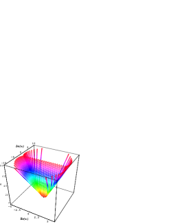
8.3 Dynamics of the zeros from Analytic Continuation

Bernoulli polynomial $B_{n}(w)$ is a polynomial of degree $n$. Thus, $B_{n}(w)$ has $n$ zeros and $B_{n+1}(w)$ has $(n+1)$ zeros. When discrete $n$ is analytic continued to continuous parameter s๐‘ s, it naturally leads to the question:

How does Bโ€‹(s,w)๐ต๐‘ ๐‘คB(s,w), the analytic continuation of $B_{n}(w)$, pick up an additional zero as s๐‘ s increases continuously by one?

This introduces the exciting concept of the dynamics of the zeros of analytic continued polynomials โ€” the idea of looking at how the zeros move about in the $\,w\,$ complex plane as we vary the parameter s๐‘ \,s\,.

Continuity shows that the additional zero simply โ€œflows in from infinityโ€.

To have a physical picture of the motion of the zeros in the complex $w$ plane, imagine that each time as s๐‘ s increases gradually and continuously by one, an additional real zero flies in from positive infinity along the real positive axis, gradually slowing down as if โ€œit is flying through a viscous mediumโ€.

For s<5๐‘ 5s<5, the additional zero simply joins onto the almost regularly spaced array of the real zeros streaming slowly towards the negative real direction. The array of zeros continue to drift freely until one by one they hit a bounding envelope which grows in size with s๐‘ s.

As s๐‘ s approaches every integer $>5$, an interesting phenomenon occurs: A pair of real zeros may meet and become a doubly degenerate real zero at a point, and then bifurcate into a pair of complex zeros conjugate to each other. Thus, the pair of real zeros appears to โ€œcollide head-on and scatter perpendicularlyโ€ into a pair of complex zeros.

Refer to captionRefer to captionRefer to captionRefer to captionRefer to captionRefer to captionRefer to captionRefer to caption\!\!\!\!\!\!\!\!\!\!\begin{array}[]{rl}\raisebox{23.0pt}{\psfig{height=162.0pt}}&\psfig{height=208.0pt}\\ \raisebox{50.0pt}{\psfig{height=103.0pt}}&\;\;\;\;\psfig{height=198.0pt}\end{array}

Figure 9: The flow of zeros of Bโ€‹(s,w)๐ต๐‘ ๐‘คB(s,w) forms a complex 3-D structure.

3 fundamental kinds of scattering can be observed:

Refer to captionRefer to captionRefer to caption(a)โ€‹ย Point(b)โ€‹ย Loop(c)โ€‹ย Long-rangeRefer to captionRefer to captionRefer to caption๐‘Žย Point๐‘ย Loop๐‘ย Long-range\begin{array}[]{ccc}\!\!\!\!\!\!\!\!\!\psfig{height=128.0pt}&\psfig{height=128.0pt}&\psfig{height=128.0pt}\\ (a)\mbox{ Point}&(b)\mbox{ Loop}&(c)\mbox{ Long-range}\end{array}

Figure 10: 3 fundamental kinds of scattering.
  • โ€ข

    Point scattering:
    A pair of real zeros scatter at a point into a pair of complex zeros which head away from each other indefinitely.

  • โ€ข

    Loop scattering:
    The same as point scattering but the pair of complex zeros loops back to recombine into degenerate real zeros within unit interval in s๐‘ s and then scatter back into a pair of real zeros, much like the picture of pair production and annihilation of virtual particles.

  • โ€ข

    Long-range sideways scattering:
    The additional zero that flies in appears as if โ€œit is carrying with it a line front of shockwaveโ€ that stretches parallelly to the $\mbox{\sf Im}(w)$ axis. When the โ€œshockwaveโ€ meets a pair of complex zeros that are looping back, the pair gets deflected away from each other momentarily before looping back again, while the additional zero gets perturbed and slows down discontinuously.

The whole complex structure can then be reduced to simple combinations of these 3 kinds of scattering.

Refer to captionRefer to caption\begin{array}[]{c}\psfig{height=128.0pt}\end{array}

Figure 11: A composite of Point, Loop and Long-range scatterings.

The movies (animated gifs) showing the motion of zeros in the complex $w$ plane at slices of s๐‘ s can be downloaded from Internet at [11] and viewed with Netscape or Internet Explorer WWW browser.

8.4 Open Challenges in Generalization

  1. 1.

    Generalize the above results of Bโ€‹(s,w)๐ต๐‘ ๐‘ค\,B(s,w)\; consistently from sโˆˆR,sโ‰ฅ1formulae-sequence๐‘ R๐‘ 1\,s\in\mbox{\sf R}\;,\;s\geq 1\; to sโˆˆC๐‘ C\,s\in\mbox{\sf C}\,.

  2. 2.

    Derive a set of expressions which give the values of s๐‘ \,s\, where the point, loop and long-range scatterings occur.

9 Conclusion

Bernoulli numbers and polynomials appear in many areas. In particular, if we assume the Riemann Hypothesis, when sโˆˆ๐‘ absents\in\,C, โ€†(23) should converge to zero only on the line s=1/2ยฑiโ€‹t๐‘ plus-or-minus12๐‘–๐‘ก\,s=1/2\pm i\/t. This remains to be proved. More of this aspect is analysed in [10].

To further self-explore these fascinating properties, feel free to download and adapt the executable Mathematica codes from [12]. Have fun!

In the meantime, it would be interesting to imagine what Jakob Bernoulli and Euler would say on these analytic continuations of their numbers and polynomials.


Acknowledgement

Special thanks to Y.L. Loh, W. Ballman, B. Lui, P. Dโ€™Eath, and K. Odagiri for discussion, all the friends in Cambridge for encouragement, and Trinity College and UK Committee of Vice-Chancellors and Principals (CVCP) for financial support.

References

  • [1] J. Bernoulli, โ€œArs Conjectandiโ€
  • [2] H. Bateman, Higher Transcendental Functions, Vol 1., (McGraw-Hill, 1953).
  • [3] M. Abramowitz and I. Stegun, Handbook of Mathematical Functions, (Dover, 1970).
  • [4] S.C. Woon, Math. Mag. 70(1), 51 (1997).
  • [5] M. Spivak, Calculus, (Benjamin, 1967), 482, Problem 17.
  • [6] E.C. Titchmarsh, The Theory of the Riemann zeta-function, (Oxford, 1986).
  • [7] S.C. Woon, Chaos Solitons & Fractals 5(1), 125 (1995).
  • [8] P. Ribenboim, The little book of Big Primes, (Springer-Verlag, 1991).
  • [9] S.C. Woon, โ€œAnalytic Continuation of Operators โ€” Operators acting complex s-timesโ€, e-Print hep-th/9707206 .
  • [10] S.C. Woon, โ€œChaos, Order, and 2 Constants in the Riemann Zeta Functionโ€, (e-Print archive chao-dyn, in preparation).
  • [11] S.C. Woon, Movies of scattering zeros, (1997)
    http://www.damtp.cam.ac.uk/user/scw21/papers/97051/movie.html
  • [12] S.C. Woon, Mathematica codes, (1997)
    http://www.damtp.cam.ac.uk/user/scw21/papers/97051/codes.html

Appendix:

Number of real and complex zeros of $B_{n}(w)$

Bnโ€‹(x)rโ€‹eโ€‹aโ€‹lcโ€‹oโ€‹mโ€‹pโ€‹lโ€‹eโ€‹xdโ€‹eโ€‹gโ€‹rโ€‹eโ€‹ezโ€‹eโ€‹rโ€‹oโ€‹szโ€‹eโ€‹rโ€‹oโ€‹snzRโ€‹(n)zCโ€‹(n)1102203304405506247348449541064117412481358146815781688175121861219712208122191222616237162481625916261016Bnโ€‹(x)rโ€‹eโ€‹aโ€‹lcโ€‹oโ€‹mโ€‹pโ€‹lโ€‹eโ€‹xdโ€‹eโ€‹gโ€‹rโ€‹eโ€‹ezโ€‹eโ€‹rโ€‹oโ€‹szโ€‹eโ€‹rโ€‹oโ€‹snzRโ€‹(n)zCโ€‹(n)27720288202992030102031112032122033924341024351124361224371324381028391128401228411328421428431132441232451332461432471532481236491336501436511536521636531736Bnโ€‹(x)rโ€‹eโ€‹aโ€‹lcโ€‹oโ€‹mโ€‹pโ€‹lโ€‹eโ€‹xdโ€‹eโ€‹gโ€‹rโ€‹eโ€‹ezโ€‹eโ€‹rโ€‹oโ€‹szโ€‹eโ€‹rโ€‹oโ€‹snzRโ€‹(n)zCโ€‹(n)541440551540561640571740581840591544601644611744621844631944641648651748661848671948682048691752701852711952722052732152742252751956762056772156782256792356802060โ‹ฎโ‹ฎโ‹ฎmissing-subexpressionmissing-subexpressionmissing-subexpressionsubscript๐ต๐‘›๐‘ฅ๐‘Ÿ๐‘’๐‘Ž๐‘™๐‘๐‘œ๐‘š๐‘๐‘™๐‘’๐‘ฅ๐‘‘๐‘’๐‘”๐‘Ÿ๐‘’๐‘’๐‘ง๐‘’๐‘Ÿ๐‘œ๐‘ ๐‘ง๐‘’๐‘Ÿ๐‘œ๐‘ ๐‘›subscriptzR๐‘›subscriptzC๐‘›missing-subexpressionmissing-subexpressionmissing-subexpressionmissing-subexpressionmissing-subexpressionmissing-subexpression110220330440550missing-subexpressionmissing-subexpressionmissing-subexpression62473484495410641174missing-subexpressionmissing-subexpressionmissing-subexpression12481358146815781688missing-subexpressionmissing-subexpressionmissing-subexpression1751218612197122081221912missing-subexpressionmissing-subexpressionmissing-subexpression22616237162481625916261016missing-subexpressionmissing-subexpressionmissing-subexpressionmissing-subexpressionmissing-subexpressionmissing-subexpressionsubscript๐ต๐‘›๐‘ฅ๐‘Ÿ๐‘’๐‘Ž๐‘™๐‘๐‘œ๐‘š๐‘๐‘™๐‘’๐‘ฅ๐‘‘๐‘’๐‘”๐‘Ÿ๐‘’๐‘’๐‘ง๐‘’๐‘Ÿ๐‘œ๐‘ ๐‘ง๐‘’๐‘Ÿ๐‘œ๐‘ ๐‘›subscriptzR๐‘›subscriptzC๐‘›missing-subexpressionmissing-subexpressionmissing-subexpressionmissing-subexpressionmissing-subexpressionmissing-subexpression277202882029920301020311120321220missing-subexpressionmissing-subexpressionmissing-subexpression33924341024351124361224371324missing-subexpressionmissing-subexpressionmissing-subexpression381028391128401228411328421428missing-subexpressionmissing-subexpressionmissing-subexpression431132441232451332461432471532missing-subexpressionmissing-subexpressionmissing-subexpression481236491336501436511536521636531736missing-subexpressionmissing-subexpressionmissing-subexpressionmissing-subexpressionmissing-subexpressionmissing-subexpressionsubscript๐ต๐‘›๐‘ฅ๐‘Ÿ๐‘’๐‘Ž๐‘™๐‘๐‘œ๐‘š๐‘๐‘™๐‘’๐‘ฅ๐‘‘๐‘’๐‘”๐‘Ÿ๐‘’๐‘’๐‘ง๐‘’๐‘Ÿ๐‘œ๐‘ ๐‘ง๐‘’๐‘Ÿ๐‘œ๐‘ ๐‘›subscriptzR๐‘›subscriptzC๐‘›missing-subexpressionmissing-subexpressionmissing-subexpressionmissing-subexpressionmissing-subexpressionmissing-subexpression541440551540561640571740581840missing-subexpressionmissing-subexpressionmissing-subexpression591544601644611744621844631944missing-subexpressionmissing-subexpressionmissing-subexpression641648651748661848671948682048missing-subexpressionmissing-subexpressionmissing-subexpression691752701852711952722052732152742252missing-subexpressionmissing-subexpressionmissing-subexpression751956762056772156782256792356missing-subexpressionmissing-subexpressionmissing-subexpression802060โ‹ฎโ‹ฎโ‹ฎmissing-subexpressionmissing-subexpressionmissing-subexpressionmissing-subexpressionmissing-subexpression\begin{array}[]{lll}\!\!\!\!\!\!\!\!\!\!\!\!\!\!\begin{array}[]{||c|c|c||}\hline\cr B_{n}(x)&real&complex\\ degree&zeros&zeros\\ n&\mbox{\bf z}_{\mbox{\scriptsize\sf R}(n)}&\mbox{\bf z}_{\mbox{\scriptsize\sf C}(n)}\\ \hline\cr\hline\cr 1&1&0\\ 2&2&0\\ 3&3&0\\ 4&4&0\\ 5&5&0\\ \hline\cr 6&2&4\\ 7&3&4\\ 8&4&4\\ 9&5&4\\ 10&6&4\\ 11&7&4\\ \hline\cr 12&4&8\\ 13&5&8\\ 14&6&8\\ 15&7&8\\ 16&8&8\\ \hline\cr 17&5&12\\ 18&6&12\\ 19&7&12\\ 20&8&12\\ 21&9&12\\ \hline\cr 22&6&16\\ 23&7&16\\ 24&8&16\\ 25&9&16\\ 26&10&16\\ \hline\cr\hline\cr\end{array}\quad\begin{array}[]{||c|c|c||}\hline\cr B_{n}(x)&real&complex\\ degree&zeros&zeros\\ n&\mbox{\bf z}_{\mbox{\scriptsize\sf R}(n)}&\mbox{\bf z}_{\mbox{\scriptsize\sf C}(n)}\\ \hline\cr\hline\cr 27&7&20\\ 28&8&20\\ 29&9&20\\ 30&10&20\\ 31&11&20\\ 32&12&20\\ \hline\cr 33&9&24\\ 34&10&24\\ 35&11&24\\ 36&12&24\\ 37&13&24\\ \hline\cr 38&10&28\\ 39&11&28\\ 40&12&28\\ 41&13&28\\ 42&14&28\\ \hline\cr 43&11&32\\ 44&12&32\\ 45&13&32\\ 46&14&32\\ 47&15&32\\ \hline\cr 48&12&36\\ 49&13&36\\ 50&14&36\\ 51&15&36\\ 52&16&36\\ 53&17&36\\ \hline\cr\hline\cr\end{array}\quad\begin{array}[]{||c|c|c||}\hline\cr B_{n}(x)&real&complex\\ degree&zeros&zeros\\ n&\mbox{\bf z}_{\mbox{\scriptsize\sf R}(n)}&\mbox{\bf z}_{\mbox{\scriptsize\sf C}}(n)\\ \hline\cr\hline\cr 54&14&40\\ 55&15&40\\ 56&16&40\\ 57&17&40\\ 58&18&40\\ \hline\cr 59&15&44\\ 60&16&44\\ 61&17&44\\ 62&18&44\\ 63&19&44\\ \hline\cr 64&16&48\\ 65&17&48\\ 66&18&48\\ 67&19&48\\ 68&20&48\\ \hline\cr 69&17&52\\ 70&18&52\\ 71&19&52\\ 72&20&52\\ 73&21&52\\ 74&22&52\\ \hline\cr 75&19&56\\ 76&20&56\\ 77&21&56\\ 78&22&56\\ 79&23&56\\ \hline\cr 80&20&60\\ \vdots&\vdots&\vdots\\ \hline\cr\hline\cr\end{array}\end{array}

Solutions of $B_{n}(w)=0$

$\begin{array}[]{||c|l||}\hline\cr\bigg{.}\mbox{ odd }n&\quad\quad\quad\quad\quad\quad\quad\quad\quad\quad w\\ \hline\cr\hline\cr 1&\begin{array}[]{l}\displaystyle\left(\frac{1}{2}\right)\end{array}\\ &\\ 3&\begin{array}[]{l}\displaystyle\left(\bigg{.}0\right),\;\left(\frac{1}{2}\right),\;\left(\bigg{.}1\right)\end{array}\\ &\\ 5&\begin{array}[]{l}\displaystyle\left(\bigg{.}0\right),\;\left(\frac{1}{2}\right),\;\left(\bigg{.}1\right),\\ \displaystyle\left(\frac{1}{2}-\frac{\sqrt{7/3}}{2}\right)\approx-0.26376,\;\left(\frac{1}{2}+\frac{\sqrt{7/3}}{2}\right)\approx 1.26376\end{array}\\ &\\ 7&\begin{array}[]{l}\displaystyle\left(\bigg{.}0\right),\;\left(\frac{1}{2}\right),\;\left(\bigg{.}1\right),\\ \displaystyle\left(\frac{1}{2}-\frac{\sqrt{9+2\sqrt{3}\,i}}{2\sqrt{3}}\right)\approx-0.38137-0.16376\,i,\\ \displaystyle\left(\frac{1}{2}-\frac{\sqrt{9-2\sqrt{3}\,i}}{2\sqrt{3}}\right)\approx-0.38137+0.16376\,i,\\ \displaystyle\left(\frac{1}{2}+\frac{\sqrt{9-2\sqrt{3}\,i}}{2\sqrt{3}}\right)\approx\;\;\,1.38137-0.16376\,i,\\ \displaystyle\left(\frac{1}{2}+\frac{\sqrt{9+2\sqrt{3}\,i}}{2\sqrt{3}}\right)\approx\;\;\,1.38137+0.16376\,i\end{array}\\ \hline\cr\hline\cr\end{array}$ $\begin{array}[]{||c|l||}\hline\cr\bigg{.}\mbox{even }n&\quad\quad\quad\quad\quad\quad\quad\quad\quad\quad w\\ \hline\cr\hline\cr 2&\begin{array}[]{l}\displaystyle\left(\frac{1}{2}-\frac{1}{2\sqrt{3}}\right)\approx 0.21133,\;\left(\frac{1}{2}+\frac{1}{2\sqrt{3}}\right)\approx 0.78868\end{array}\\ &\\ 4&\begin{array}[]{l}\displaystyle\left(\frac{1}{2}-\frac{\sqrt{15+2\sqrt{30}}}{2\sqrt{15}}\right)\approx-0.15770,\\ \displaystyle\left(\frac{1}{2}-\frac{\sqrt{15-2\sqrt{30}}}{2\sqrt{15}}\right)\approx\;\;\,0.24034,\\ \displaystyle\left(\frac{1}{2}+\frac{\sqrt{15-2\sqrt{30}}}{2\sqrt{15}}\right)\approx\;\;\,0.75967,\\ \displaystyle\left(\frac{1}{2}+\frac{\sqrt{15+2\sqrt{30}}}{2\sqrt{15}}\right)\approx\;\;\,1.15770\end{array}\\ \hline\cr\hline\cr\end{array}$