Simulating Plasma Turbulence in Tokamaks
The development of magnetic fusion energy is a continuing national priority. Present day toroidally confined plasma experiments (tokamaks) are producing fusion power comparable to the input power needed to heat the plasma (). One of the basic physics problems is to understand turbulent transport phenomena, which cause particles and energy to escape the confining magnetic fields. Plasma turbulence is challenging from a theoretical point of view because of the nonlinearity and high dimensionality of the governing equations. Experimental measurements in the core region of a tokamak are limited by the extremely high temperatures, Kelvin, of the confined plasma. The high levels of both theoretical and experimental difficulty highlight the potentially important role of numerical simulations in developing a predictive model for turbulent transport. Such a model would dramatically reduce uncertainties in tokamak design and could lead to enhanced operating regimes, both of which would reduce the size and expense of a fusion reactor.
An understanding of turbulent transport and the exploration of modes of operation that suppress turbulence are central goals of the numerical tokamak project, one of the Grand Challenges of the national HPCC program. The process of modeling entails three main steps: (1) the development of a simplified model of tokamaks that encompasses the essential physics of the relevant instabilities, (2) the creation of numerical algorithms for solving the governing equations, and (3) implementation of these methods on massively parallel architectures. This third step is necessary if we are to achieve simulations of sufficient size and resolution to explain the trends seen in experiments.
The state of the plasma is given by the distribution function , whose evolution is described by the gyrokinetic equations—a reduced set of equations derived from the Vlasov equation by phase averaging over the ion gyromotion while keeping only the relevant temporal and spatial scales [3, 6]. This averaging of the fast gyromotion reduces the dimensionality of the governing equations from six to five. In addition, recently developed numerical methods make it possible to follow only the perturbations of the distribution function from a stationary equilibrium (see [10] and references therein). Even with the considerable complexity of the gyrokinetic equations and the so-called “ method,” the algorithms are analogous to those used in conventional particle-in-cell (PIC) simulations. PIC codes are both memory- and CPU-intensive, and the effective use of high performance computing, in particular massively parallel architectures, which require a domain decomposition of the problem, is essential for the success of the numerical tokamak project. Fortunately, this problem lends itself naturally to a one-dimensional decomposition.
As an example of a few partially realized goals of the numerical tokamak project, we present here some recent results for the simulation of modes that may act as barriers to turbulent transport. Our three-dimensional gyrokinetic simulation code is being used to study two effects that are linearly stabilizing and that may cause the formation of transport barriers: reversed magnetic shear and peaked density profiles [11]. We have found that weak or negative magnetic shear, in combination with a peaked density profile relative to the temperature profile, greatly suppresses turbulence in the central region of the simulations. Similar features have been seen experimentally [7].
Tokamak Geometry
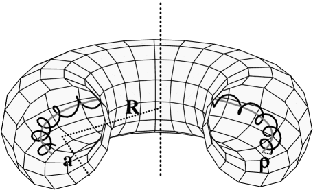
The essential geometry of a tokamak is that of a torus defined by a major radius and a minor radius (see Figure 1). The ions within the plasma move rapidly around the torus, gyrating tightly along the magnetic field lines, like rings on a wire. The radius of the gyration is , where is the transverse velocity and is the gyro frequency, with being the charge, the magnetic field strength, the particle mass, and the speed of light. The essential scale (resolution) of the system (simulation) is set by . Typically cm, cm, and cm.
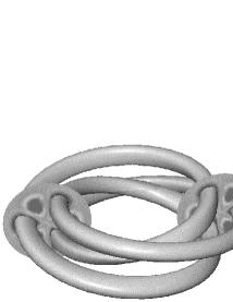
The simplest arrangement of field lines is obtained by wrapping current-carrying wires tightly around the minor axis of the torus, creating straight magnetic field lines aligned with the torus. Unfortunately, the magnetic field exerts a greater force on the inside of the torus, which causes the ions in the plasma to drift across the field lines. This problem can be partially alleviated by twisting the field lines into a helical shape in such a way that the drifts approximately cancel. A byproduct of the twisting is that the particle trajectories become far more complex and are increasingly susceptible to a wide range of instabilities, which tend to grow along the toroidal modes of the tokamak. Figure 2 shows a simplified example of a typical toroidal mode—an , mode ( is the poloidal mode number, and is the toroidal mode number). This could be, for example, the linear growth phase of an ion density perturbation. The linear phase of an instability in realistic plasmas typically has much larger values for and (10–100), but a similar helical twist (the ratio ). In addition, the realistic case has a sheared magnetic geometry (i.e., a radially varying amount of helical twist in the magnetic field lines). Generally, the isosurfaces of a perturbation follow the helical shape of the magnetic field lines.
Governing Equations
The governing gyrokinetic equations are phase space conserving and have the same form as the Vlasov equation:
where , with being the guiding center position of the gyrating particle, the particle’s velocity along the magnetic field line, and a constant of motion that parameterizes the particle’s velocity perpendicular to the magnetic field.
The electrostatic toroidal gyrokinetic equations used for all the results discussed here are those derived by Hahm [4]. Because the variations in are quite small, (%) is used to carry out a perturbative expansion. in the expansion is solved by integrating the characteristics of the resulting gyrokinetic equations. More details can be found in [9] and in references therein. It is important to realize that although the solution of these equations is algorithmically analogous to the solution of plus Maxwell’s equations, much theoretical care and effort has been devoted to simplifying the problem while retaining the important physics. Simplifications include reduction of the dimensionality, elimination of short space–time scales, and reduction of particle simulation noise.
Numerical Method and Parallel Implementation
Particle-in-cell simulation has been used in the plasma physics community for several decades. The general idea is that the particles interact with both self-created and externally imposed electromagnetic fields. The code thus has two distinct parts and data structures. For illustration purposes, we consider the conventional electrostatic equations, which retain the essence of the algorithm [2]. The trajectories of particles with mass and charge are given by
where the subscript refers to the -th particle. The algorithm generally used to solve this set of equations is a time-centered leapfrog scheme,
where the electric field at the particle’s position is found by interpolation from electric fields previously calculated on a grid. The interpolation, a gather operation that involves indirect addressing, accounts for a substantial part of the computation time.
In the second part of the code, the fields created by the particles must be found from Poisson’s equation,
with and the sum being over each type of particle species. Fourier transform methods are used to solve this equation on a grid. Typically, the time for the field solver is not large. The source term is calculated from the particle position by an inverse interpolation,
where is a particle shape function. This is a scatter operation that also involves indirect addressing and consumes a substantial part of the calculation time.
Since the dominant part of the calculation in a particle code involves interpolation between particles and grids, it is important for a parallel implementation that these two data structures reside on the same processor. Different processors are assigned different regions of space, and particles are assigned to processors according to their locations [8]. As particles move from one region to another, they are moved to the processor associated with the new region. Because particles must also access neighboring regions of space during the interpolation, extra guard cells are kept in each processor, to be combined or replicated as needed after the particles are processed. The passing of particles from one processor to another is performed by a particle-manager subroutine. The passing of field data between guard cells is performed by a field-manager subroutine.
The field solver uses Fourier transform methods. There are two FFTs per timestep, one for the charge density and one for the electric potential. A parallel complex-to-complex FFT was developed with a transform method in which the coordinate local to the processor is transformed first, the data are then transposed so that the coordinate that was distributed becomes local, and, finally, the remaining coordinate is transposed. The maximum number of processors that can be used is limited by the maximum number of grid points in any one coordinate, but this is not a severe constraint at present since the numerical tokamak is designed for systems in which this number is about 512.
During the transpose phase of the FFT, each processor sends one piece of data to every other processor. This can be accomplished in a number of ways, but the safest is always to have one message sent, one message received, and so on. Flooding the computer with large numbers of simultaneous messages tends to overflow system resources and is not always reliable.
The structure of the main loop of the simplified code is summarized as follows:
-
1.
Particle coordinates are updated by an acceleration subroutine.
-
2.
Particles are moved to neighboring processors by a particle-manager subroutine.
-
3.
Particle charge is deposited on the grid by a deposit subroutine.
-
4.
Guard cells are combined by a field-manager subroutine.
-
5.
Complex-to-complex FFT of charge density is performed by an FFT subroutine.
-
6.
Electric potential is found in Fourier space by a Poisson solver subroutine.
-
7.
Complex-to-complex FFT of electric potential is performed by an FFT subroutine.
-
8.
Electric potential is distributed to guard cells by a field-manager subroutine.
This structure has the beneficial feature that the physics modules, items 1, 3, and 6, contain no communication calls (except for a single call to sum energies across processors). These modules can easily be modified by researchers who do not have special knowledge of parallel computing or message passing. The communications modules, items 2, 4, and 8, handle data management but do not perform any calculation, and can be used by physicists as black boxes, where only the input and output must be understood. The FFT, items 5 and 7, are the usual sequential FFTs, with an additional embedded transpose subroutine, which can also be used as a black box. Furthermore, since most message-passing libraries are quite similar, moving from one distributed-memory computer to another simply involves replacing the message-passing calls in the communications modules with new ones.
General Behavior
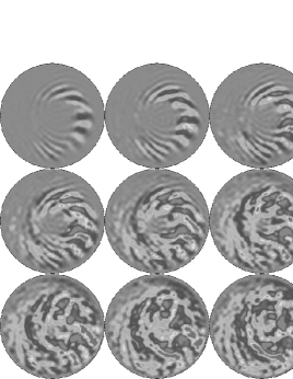
When a simulation starts with a very small initial perturbation, the run generally has two identifiable phases. The first is the linear phase, where modes (i.e., standing waves) grow exponentially. Lower-dimensional, time-independent eigenvalue techniques that are fairly well understood theoretically can also be used to find linear modes. The second phase is the turbulent stationary state, during which the growth of the dominant linear modes saturates and the system settles down to a statistical steady state. The transition from linear to turbulent behavior is demonstrated in Figure 3.
Parallel Performance
In our implementation, we use a one-dimensional domain decomposition along the toroidal axis, which is generally more efficient and significantly easier to program than a full three-dimensional decomposition. In addition, the number of particles per processor remains relatively constant along this axis, which minimizes load imbalance. Furthermore, since the mean flow of the particles has been subtracted off in the perturbation expansion, the particles themselves do not move rapidly across cells, which keeps the communication low. For these reasons, we would expect to get excellent parallel performance.
In the most recent efforts, Fortran 77 and the PVM message-passing library have been used to port the code to the Cray T3D [1]. Production runs on the T3D show a performance of approximately 14.4 MFlops per processor (10% of the theoretical peak of 150 MFlops, which is typical for applications of this type). To test the scalability of the code, 12 runs were timed with different numbers of processors and problem sizes. These times, along with the parameters of the runs, are shown in Table 1.
| No. of | grid | particles | No. of | wallclock | speed (msec-processor |
|---|---|---|---|---|---|
| particles | size | /grid cell | processors | sec/step | /particles-step) |
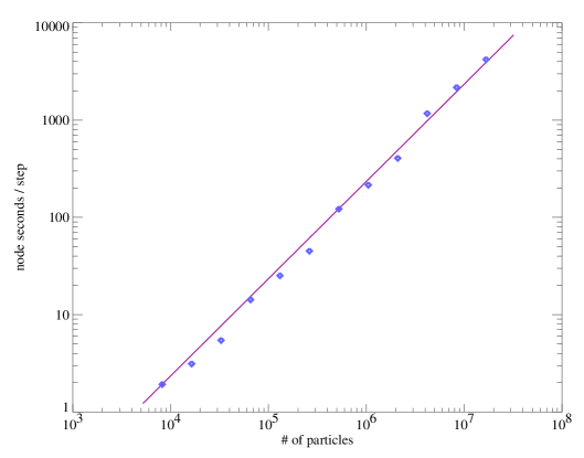
To first order, the problem size is given by the total number of particles. The total amount of computer resources consumed is the time per step multiplied by the number of processors. These two quantities are plotted in Figure 4. In a perfectly scalable code, which is represented by the straight line in Figure 4, the resource consumption should be proportional to the problem size. What is most impressive is that the full code, with all diagnostics and outputs, was used to obtain these results. Simply put, this means that doubling the number of CPUs or halving the size of the problem will halve the computation time. In addition, it is worth mentioning that the code has a very low communication/computation ratio (). This ratio is a rough measure of the fraction of time spent waiting for processors to transmit information, and the low value for our program is an indication that it can be expected to perform well if even more processors or faster processors are used. This is encouraging because the Cray T3E will have processors that are significantly faster.
Simulating Transport Barriers
Transport barriers in tokamaks have been an important aspect in a host of operational modes, such as the H-mode, where edge transport is thought to be greatly reduced through poloidal shear flow. In the recent enhanced reverse shear experiments on TFTR [7], it has been reported that density and ion heat transport are below conventional neoclassical levels in the core. Comprehensive linear calculations [5, 12] show this region to be locally stable to micro-instabilities. New gyrokinetic simulations presented here show that the combined effects of reversed magnetic shear and a peaked density profile allow for a good confinement zone in the core region [11]. Figure 5 shows the difference in energy flux for simulations with and without reversed magnetic shear and a peaked density profile. These new results are differ with past simulations (that did not include these effects), which have generally shown a global (slow) relaxation of the temperature profile.

Future Work
Future directions for this work include the incorporation of more detailed physics, such as an electron model that includes a trapped component and studies of the effects of magnetic perturbations. Ultimately, the goal is to understand plasma turbulence at a level that is detailed enough to allow quantitative predictions of heat transport. This will reduce uncertainties in design, and hence the cost, of future tokamak reactors. As shown here, progress toward this long-term goal can be made through close interaction between theory and direct numerical simulation.
Acknowledgments
The authors especially thank J. Cummings, W.W. Lee, H. Mynick, R. Samtaney, E. Valeo, and N. Zabusky. Much of this work was carried out at the Princeton Plasma Physics Laboratory as an active part of the community-wide Numerical Tokamak Project supported through the HPCC Initiative. Computing resources were provided by JPL at Caltech, ACL at LANL, NERSC at LLNL, and the Pittsburgh Supercomputing Center. This work is supported by the U.S. Department of Energy, through Contract DE-AC02-76CHO-3073, Grant DE-FG02-93ER25179.A000, and the Computational Science Graduate Fellowship Program.
References
- [1] V.K. Decyk, How to write (nearly) portable Fortran programs for parallel computers, Computers in Physics, 7(1993), pp. 418–424.
- [2] V.K. Decyk, Skeleton PIC codes for parallel computers, Computer Physics Communications, 87(1995), pp. 87–94.
- [3] E.A. Frieman and L. Chen, Nonlinear gyrokinetic equations for low-frequency electromagnetic waves in general plasma equilibrium, Physics of Fluids, 25(1982), pp. 502–507.
- [4] T.S. Hahm, Nonlinear gyrokinetic equations for tokamak microturbulence, Physics of Fluids, 31(1988), pp. 2670–2673.
- [5] C. Kessel, J. Manickam, G. Rewoldt, and W.M. Tang, Improved plasma performance in tokamaks with negative magnetic shear, Physical Review Letters, 72(1994), pp. 1212–1215.
- [6] W.W. Lee, Gyrokinetic particle simulation model, Journal of Computational Physics, 72(1987), pp. 243–269.
- [7] F.M. Levinton, et.al., Improved confinement with reversed magnetic shear in TFTR, Physical Review Letters, 75(1995), pp. 4417–4420.
- [8] P.C. Liewer, V.K. Decyk, and A. de Boer, A general concurrent algorithm for plasma particle-in-cell simulation codes, Journal of Computational Physics, 85(1989), pp. 302–322.
- [9] S.E. Parker, W.W. Lee and R.A. Santoro, Gyrokinetic simulation of ion temperature gradient driven turbulence in 3D toroidal geometry, Physical Review Letters, 71(1993), pp. 2042–2045.
- [10] S.E. Parker and W.W. Lee, A fully nonlinear characteristic method for gyrokinetic simulation, Physics of Fluids B, 5(1993), pp. 77–86.
- [11] S.E. Parker, H.E. Mynick, M. Artun, J.C. Cummings, V. Decyk, J.V. Kepner, W.W. Lee, and W.M. Tang, Radially global gyrokinetic simulation studies of transport barriers, Physics of Plasmas, 3(1996), pp. 1959–1966.
- [12] G.W. Rewoldt and W.M. Tang, private communication, 1995.
Jeremy Kepner (jvkepner@astro.princeton.edu) is a graduate student in the Department of Astrophysics at Princeton University. Scott Parker (sparker@buteo.colorado.edu) is a professor in the Department of Physics at the University of Colorado in Boulder. Viktor Decyk (vdecyk@pepper.physics.ucla.edu) is a research scientist in the Department of Physics at the University of California in Los Angeles.