MUON-MUON AND OTHER HIGH ENERGY COLLIDERS

Center for Accelerator Physics
Brookhaven National Laboratory
Upton, NY 11973-5000, USA

0.1 COMPARISON OF COLLIDER TYPES

0.1.1 Introduction

Before we discuss the muon collider in detail, it is useful to look at the other types of colliders for comparison. In this chapter we consider the high energy physics advantages, disadvantages and luminosity requirements of hadron ($pp$, $p\bar{p}$), of lepton ($e^{+}e^{-}$, $\mu^{+}\mu^{-}$ ) and photon-photon colliders. Technical problems in obtaining increased energy in each type of machine are presented. Their relative size, and probable relative costs are discussed.

0.1.2 Physics Considerations

General.

Hadron-hadron colliders ($pp$  or $p\bar{p}$) generate interactions between the many constituents of the hadrons (gluons, quarks and antiquarks); the initial states are not defined and most interactions occur at relatively low energy, generating a very large background of uninteresting events. The rate of the highest energy events is higher for antiproton-proton machines, because the antiproton contains valence antiquarks that can annihilate on the quarks in the proton. But this is a small effect for colliders above a few TeV, when the interactions are dominated by interactions between quarks and antiquarks in their seas, and between the gluons. In either case the individual parton-parton interaction energies (the energies used for physics) are a relatively small fraction of the total center of mass energy. This is a disadvantage when compared with lepton machines. An advantage, however, is that all final states are accessible. Many, if not most, initial discoveries in Elementary Particle Physics have been made with these machines.

In contrast, lepton-antilepton collider generate interactions between the fundamental point-like constituents in their beams, the reactions generated are relatively simple to understand, the full machine energies are available for “physics”, and there is negligible background of low energy events. If the center of mass energy is set equal to the mass of a suitable state of interest, then there can be a large cross section in the s-channel, in which a single state is generated by the interaction. In this case, the mass and quantum numbers of the state are constrained by the initial beams. If the energy spread of the beams is sufficiently narrow, then precision determination of masses and widths are possible.

A gamma-gamma collider, like the lepton-antilepton machines, would also have all the machine energy available for physics, and would have well defined initial states, but these states would be different from those with the lepton machines, and thus be complementary to them.

For most purposes (technical considerations aside) $e^{+}e^{-}$and $\mu^{+}\mu^{-}$ colliders would be equivalent. But in the particular case of s-channel Higgs boson production, the cross section, being proportional to the mass squared, is more than 40,000 times greater for muons than electrons. When technical considerations are included, the situation is more complicated. Muon beams are harder to polarize and muon colliders will have much higher backgrounds from decay products of the muons. On the other hand muon collider interactions will require less radiative correction and will have less energy spread from beamstrahlung.

Each type of collider has its own advantages and disadvantages for High Energy Physics: they would be complementary.

Required Luminosity for Lepton Colliders.

In lepton machines the full center of mass of the leptons is available for the final state of interest and a “physics energy” $E_{\rm phy}$ can be defined that is equal to the total center of mass energy.

$$E_{\rm phy}\ =\ E_{c\ of\ m}$$ (2)

Since fundamental cross sections fall as the square of the center of mass energies involved, so, for a given rate of events, the luminosity of a collider must rise as the square of its energy. A reasonable target luminosity is one that would give 10,000 events per unit of R per year (the cross section for lepton pair production is one R, the total cross section is about 20 R, and somewhat energy dependent as new channels open up):

$$\cal L\rm_{req.}\ \approx\ 10^{34}\ (cm^{-2}s^{-1})\ \left({E_{phy}\over 1\ (TeV)}\right)^{2}$$ (3)

Fig. 1 shows this required luminosity, together with crosses at the approximate achieved luminosities of some lepton colliders. Target luminosities of possible future colliders are also given as circles.

Figure 1.: Luminosity of lepton colliders as a function of Energy

The Effective Physics Energies of Hadron Colliders.

Hadrons, being composite, have their energy divided between their various constituents. A typical collision of constituents will thus have significantly less energy than that of the initial hadrons. Studies done in Snowmass 82 and 96 suggest that, for a range of studies, and given the required luminosity (as defined in Eq. 3), then the hadron machine’s effective “physics” energy is between about 1/3 and 1/10 of its total. We will take a value of 1/7:

$$E_{\rm phy}(\cal L\rm=\cal L\rm_{req.})\ \approx\ {E_{c\ of\ m}\over 7}$$

The same studies have also concluded that a factor of 10 in luminosity is worth about a factor of 2 in effective physics energy, this being approximately equivalent to:

$$E_{\rm phy}(\cal L\rm)\ =\ E_{\rm phy}(\cal L\rm=\cal L\rm_{req.})\ \left({\cal L\rm\over\cal L\rm_{req}}\right)^{0.3}$$

From which, with Eq. 3, one obtains:

$$E_{\rm phy}\approx\left({E_{c\ of\ m}\over 7(TeV)}\right)^{0.6}\left({\cal L\rm\over 10^{34}(cm^{-2}s^{-1})}\right)^{0.2}(TeV)$$ (4)

Table 1.: Effective Physics Energy of Some Hadron Machines

Machine	C of M Energy	Luminosity	Physics Energy
	TeV	$cm^{-2}s^{-1}$	TeV
ISR	.056	$10^{32}$	0.02
TeVatron	1.8	$7\times 10^{31}$	0.16
LHC	14	$10^{34}$	1.5
VLHC	60	$10^{34}$	3.6

Tb. 1 gives some examples of this approximate “physics” energy. It must be emphasized that this effective physics energy is not a well defined quantity. It should depend on the physics being studied. The initial discovery of a new quark, like the top, can be made with a significantly lower “physics” energy than that given here. And the capabilities of different types of machines have intrinsic differences. The above analysis is useful only in making very broad comparisons between machine types.

0.1.3 Hadron-Hadron Machines

Luminosity.

An antiproton-proton collider requires only one ring, compared with the two needed for a proton-proton machine (the antiproton has the opposite charge to the proton and can thus rotate in the same magnet ring in the opposite direction - protons going in opposite directions require two rings with bending fields of the opposite sign), but the luminosity of an antiproton- proton collider is limited by the constraints in antiproton production. A luminosity of at least $10^{32}\ {\rm cm}^{-2}{\rm s}^{-1}$ is expected at the antiproton-proton Tevatron; and a luminosity of $10^{33}\ {\rm cm}^{-2}{\rm s}^{-1}$ may be achievable, but LHC, a proton-proton machine, is planned to have a luminosity of $10^{34}\ {\rm cm}^{-2}{\rm s}^{-1}$. Since the required luminosity rises with energy, proton-proton machines seem to be favored for future hadron colliders.

The LHC and other future proton-proton machines might even[lumlim] be upgradable to $10^{35}\ {\rm cm}^{-2}{\rm s}^{-1}$, but radiation damage to a detector would then be a severe problem. The 60 TeV Really Large Hadron Colliders (RLHC: high and low field versions) discussed at Snowmass are being designed as proton-proton machines with luminosities of $10^{34}\ {\rm cm}^{-2}{\rm s}^{-1}$ and it seems reasonable to assume that this is the highest practical value.

Size and Cost.

The size of hadron-hadron machines is limited by the field of the magnets used in their arcs. A cost minimum is obtained when a balance is achieved between costs that are linear in length, and those that rise with magnetic field. The optimum field will depend on the technologies used both for the the linear components (tunnel, access, distribution, survey, position monitors, mountings, magnet ends, etc) and those of the magnets themselves, including the type of superconductor used.

The first hadron collider, the 60 GeV ISR at CERN, used conventional iron pole magnets at a field less than 2 T. The only current hadron collider, the 2 TeV Tevatron, at FNAL, uses NbTi superconducting magnets at approximately $4\,{}^{\circ}K$ giving a bending field of about 4.5 T. The 14 TeV Large Hadron Collider (LHC), under construction at CERN, plans to use the same material at $1.8\,{}^{\circ}K$ yielding bending fields of about $8.5\,{\rm T}.$

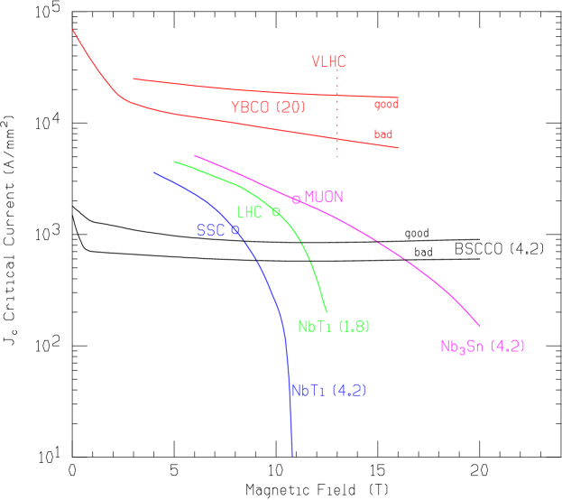
Figure 2.: Critical current densities of superconductors as a function of magnetic field.

Future colliders may use new materials allowing even higher magnetic fields. Fig. 2 shows the critical current densities of various superconductors as a function of magnetic field. The numbers in parenthesis refer to the temperatures in ^∘ K. good and bad refer to the best and worst performance according to the orientation of the tape with respect to the direction of the magnetic field. Model magnets have been made with ${\rm Nb_{3}Sn},$ and studies are underway on the use of high T_c superconductor. Bi₂Sr₂Ca₁Cu₂O₈ (BSCCO) material is currently available in useful lengths as powder-in-Ag tube processed tape. It has a higher critical temperature and field than conventional superconductors, but, even at $4\,{}^{\circ}K,$ its current density is less than ${\rm Nb_{3}Sn}$ at all fields below 15 T. It is thus unsuitable for most accelerator magnets. In contrast YBa₂Cu₃O₇ (YBCO) material has a current density above that for Nb₃Sn ($4\,{}^{\circ}K$), at all fields and temperatures below $20\,{}^{\circ}K.$ But this material must be deposited on specially treated metallic substrates and is not yet available in lengths greater than 1 m. It is reasonable to assume, however, that it will be available in useful lengths in the not too distant future.

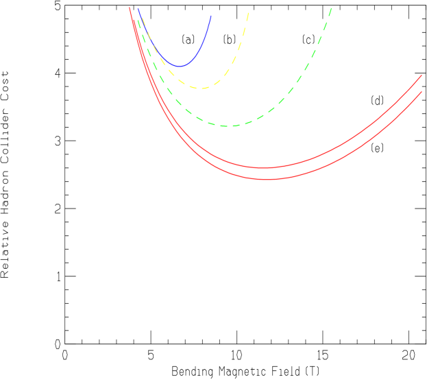
Figure 3.: Relative costs of a collider as a function of its bending magnetic field, for different superconductors and operating temperatures. Costs are given for NbTi at (a) $4\,{}^{\circ}K$, and (b) $1.8\,{}^{\circ}K$, (c) Nb₃ Sn at $4.3\,{}^{\circ}K$, and (d) and (e) YBCO High T_c at $20\,{}^{\circ}K.$ NbTi and Nb₃ Sn costs per unit weight were taken to be the same; YBCO was taken to be either equal to NbTi (in (d)), or 4 times NbTi (in (e)).

A parametric study was undertaken to learn what the use of such materials might do for the cost of colliders. 2-in-1 cosine theta superconducting magnet cross sections (in which the two magnet coils are circular in cross section, have a cosine theta current distributions and are both enclosed in a single iron yoke) were calculated using fixed criteria for margin, packing fraction, quench protection, support and field return. Material costs were taken to be linear in the weights of superconductor, copper stabilizer, aluminum collars, iron yoke and stainless steel support tube. The cryogenic costs were taken to be inversely proportional to the operating temperature, and linear in the outer surface area of the cold mass. The values of the cost dependencies were scaled from LHC estimates.

Results are shown in Fig. 3. Costs were calculated assuming NbTi at (a) $4\,{}^{\circ}K$, and (b) $1.8\,{}^{\circ}K,$ Nb₃ Sn at (c) $4.3\,{}^{\circ}K$ and YBCO High T_c at $20\,{}^{\circ}K$ (d) and (e). NbTi and Nb₃ Sn costs per unit weight were taken to be the same; YBCO was taken to be either equal to NbTi (in (d)), or 4 times NbTi (in (e)). It is seen that the optimum field moves from about 6 T for NbTi at $4\,{}^{\circ}K$ to about 12 T for YBCO at $20\,{}^{\circ}K$; while the total cost falls by almost a factor of 2.

One may note that the optimized cost per unit length remains approximately constant. This might have been expected: at the cost minimum, the cost of linear and field dependent terms are matched, and the total remains about twice that of the linear terms.

The above study assumes this particular type of magnet and may not be indicative of the optimization for radically different designs. A group at FNAL[pipe] is considering an iron dominated, alternating gradient, continuous, single turn collider magnet design (Low field RLHC). Its field would be only 2 T and circumference very large (350 km for 60 TeV), but with its simplicity and with tunneling innovations, it is hoped to make its cost lower than the smaller high field designs. There are however greater problems in achieving high luminosity with such a machine than with the higher field designs.

0.1.4 Circular $e^{+}e^{-}$Machines

Luminosity.

The luminosities of most circular electron-positron colliders has been between $10^{31}$ and $10^{32}\,{\rm cm}^{-2}{\rm s}^{-1}$ (see Fig.1), CESR is fast approaching $10^{33}\,{\rm cm}^{-2}{\rm s}^{-1}$ and machines are now being constructed with even high values. Thus, at least in principle, luminosity does not seem to be a limitation (although it may be noted that the 0.2 TeV electron-positron collider LEP has a luminosity below the requirement of Eq.3).

Size and Cost.

At energies below 100 MeV, using a reasonable bending field, the size and cost of a circular electron machine is approximately proportional to its energy. But at higher energies, if the bending field $B$ is maintained, the energy lost $\Delta V_{\rm turn}$ to synchrotron radiation rises rapidly

$$\Delta V_{\rm turn}\ \propto\ {E^{4}\over R\ m^{4}}\ \propto\ {E^{3}\ B\over m^{4}}$$ (5)

and soon becomes excessive ($R$ is the radius of the ring). A cost minimum is then obtained when the cost of the ring is balanced by the cost of the rf needed to replace the synchrotron energy loss. If the ring cost is proportional to its circumference, and the rf is proportional to its voltage then the size and cost of an optimized machine rises as the square of its energy. This relationship is well demonstrated by the parameters of actual machines as shown later in Fig. 7.

The highest circular $e^{+}e^{-}$collider is the LEP at CERN which has a circumference of 27 km, and will achieve a maximum center of mass energy of about 0.2 TeV. Using the predicted scaling, a 0.5 TeV circular collider would have to have a 170 km circumference, and would be very expensive.

0.1.5 $e^{+}e^{-}$Linear Colliders

Size and Cost.

So, for energies much above that of LEP (0.2 TeV) it is probably impractical to build a circular electron collider. The only possibility then is to build two electron linacs facing one another. Interactions occur at the center, and the electrons, after they have interacted, must be discarded.

Luminosity.

The luminosity $\cal L\rm$ of a linear collider can be written:

$$\cal L\rm\ =\ {1\over 4\pi E}\ \ {N\over\sigma_{x}}\ {P_{\rm beam}\over\sigma_{y}}\ \ n_{\rm collisions}$$ (6)

where $\sigma_{x}$ and $\sigma_{y}$ are average beam spot sizes including any pinch effects, and we take $\sigma_{x}$ to be much greater than $\sigma_{y}$. $E$ is the beam energy, $P_{\rm beam}$ is the total beam power, and, in this case, $n_{\rm collisions}=1$. This can be expressed[yokoyachen] as,

$$\cal L\rm\ \approx\ {1\over 4\pi E}\ \ {n_{\gamma}\over 2r_{o}\alpha\ U(\Upsilon)}\ \ \ \ {P_{\rm beam}\over\sigma_{y}}$$ (7)

where the quantum correction $U(\Upsilon)$ is given by

$$U(\Upsilon)\ \approx\ \sqrt{{1\over{1+\Upsilon^{2/3}}}}$$ (8)

with

$$\Upsilon\ \approx\ {2F_{2}r_{e}^{2}\over\alpha}\ {N\ \gamma\over\sigma_{z}\ \sigma_{x}}$$ (9)

$F_{2}\approx 0.43$, $r_{o}$ is the classical electromagnetic radius, $\alpha$ is the fine-structure constant, and $\sigma_{z}$ is the rms bunch length. The quantum correction $\Upsilon$ is close to unity for all proposed machines with energy less than 2 TeV, and this term is often omitted[peskin]. Even in a 5 TeV design[me], an $\Upsilon$ of 21 gives a suppression factor of only 3.

$n_{\gamma}$ is the number of photons emitted by one electron as it passes through the other bunch. If $n_{\gamma}$ is significantly greater than one, then problems are incountered with backgrounds of electron pairs and mini-jets, or with unacceptable beamstrahlung energy loss. Thus $n_{\gamma}$ can be taken as a rough criterion of these effects and constrained to a fixed value. We then find:

$$\cal L\rm\ \propto{1\over E}\ \ {P_{beam}\over\sigma_{y}\ U(\Upsilon)}$$

which may be compared to the required luminosity that increases as the square of energy, giving the requirement:

$${P_{\rm beam}\over\sigma_{y}\ U(\Upsilon)}\ \propto\ E^{3}.$$ (10)

It is this requirement that makes it hard to design very high energy linear colliders. High beam power demands high efficiencies and heavy wall power consumption. A small $\sigma_{y}$ requires tight tolerances, low beam emittances and strong final focus and a small value of $U(\Upsilon)$ is hard to obtain because of its weak dependence on $\Upsilon$ ($\propto\Upsilon^{-1/3}$).

Conventional RF.

The gradients for structures have limits that are frequency dependent. Fig. 4 shows the gradient limits from breakdown, fatigue and dark current capture, plotted against the operating rf frequency. Operating gradients and frequencies of several linear collider designs[bluebook] are also indicated.

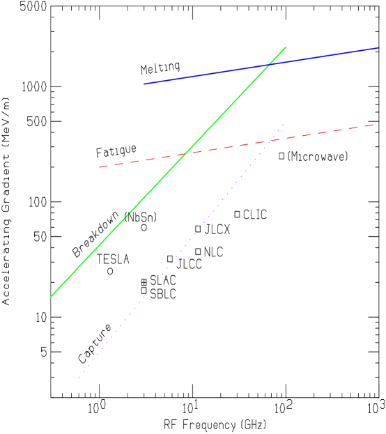
Figure 4.: Gradient values and limits in linear collider electron linacs, superconducting examples are indicated as circles

One sees that for conventional structure designs (indicated as squares in Fig. 4), the proposed gradients fall well below the limits, except for the dark current capture threshold. Above this threshold, in the absence of focusing fields, dark current electrons emitted in one cavity can be captured and accelerated down the entire linac causing loading problems. We note, however, that the superconducting TESLA design is well above this limit, and a detailed study[akasaka] has shown that the quadrupole fields in a focusing structure effectively stop the build up of such a current.

The real limit on accelerating gradients in these designs come from a trade off between the cost of rf power against the cost of length. The use of high frequencies reduces the stored energy in the cavities, reducing the rf costs and allowing higher accelerating gradients: the optimized gradients being roughly proportional to the frequency. One might thus conclude then that higher frequencies should be preferred. There are however counterbalancing considerations from the requirements of luminosity.

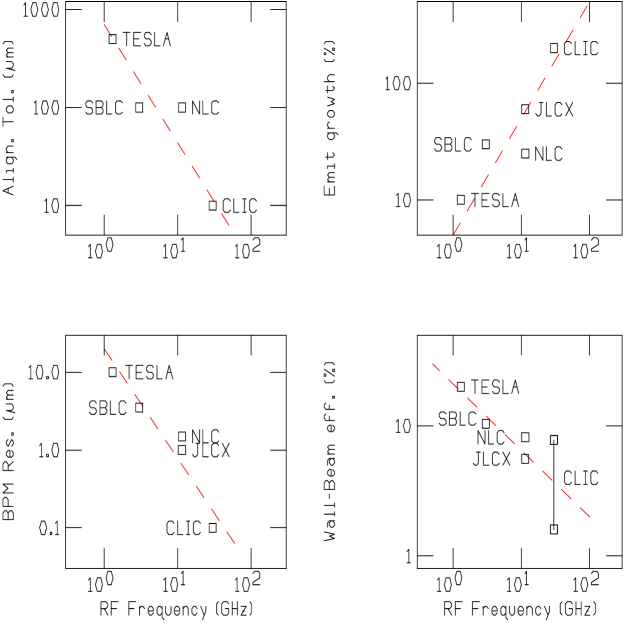
Figure 5.: Dependence of some sensitive parameters as a function of linear collider rf frequency.

Fig. 5, using parameters from the linear collider proposals [bluebook], plots some relevant parameters against the rf frequency. One sees that as the frequencies rise,

• the required alignment tolerances are tighter;

• the resolution of beam position monitors must also be better; and

• despite these better alignments, the calculated emittance growth during acceleration is worse; and

• the wall-power to beam-power efficiencies are also less.

Thus while length and cost considerations may favor high frequencies, yet luminosity considerations demand lower frequencies.

Superconducting RF.

If, however, the rf costs can be reduced, for instance when superconducting cavities are used, then there will be no trade off between rf power cost and length and higher gradients should be expected to lower the length and cost. The removal of the constraint applied by rf power considerations is evident for the TESLA gradient plotted in Fig. 4. Its value is well above the trend of conventional rf designs. Unfortunately the gradients achievable in currently operating niobium superconducting cavities is lower than that planned in the higher frequency conventional rf colliders. Theoretically the limit is about 40 MV/m, but practically 25 MV/m is as high as seems possible. Nb₃Sn and high Tc materials may allow higher field gradients in the future. A possible value for Nb₃Sn is also indicated on Fig. 4.

In either case, the removal of the requirements for huge peak rf power allows the choice of longer wavelengths (the TESLA collaboration is proposing 23 cm at 1.3 GHz) and greatly relieves the emittance requirements and tolerances, with no loss of luminosity.

At the current 25 MeV per meter gradients, the length and cost of a superconducting machine is probably higher than for the conventional rf designs. With greater luminosity more certain, its proponents can argue that it is worth it the greater price. If higher gradients become possible, using new superconductors, then the advantages of a superconducting solution could become overwhelming.

At Higher Energies.

At higher energies (as expected from Eq. 10), obtaining the required luminosity gets harder. Fig.6 shows the dependency of some example machine parameters with energy. SLC is taken as the example at 0.1 TeV, NLC parameters at 0.5 and 1 TeV, and 5 and 10 TeV examples are taken from a review paper by one of the authors[me]. One sees that:

• the assumed beam power rises approximately as $E$;

• the vertical spot sizes fall approximately as $E^{-2}$;

• the vertical normalized emittances fall even faster: $E^{-2.5}$; and

• the momentum spread due to beamstrahlung has been allowed to rise almost linearly with $E$.

These trends are independent of the acceleration method, frequency, etc, and indicate that as the energy and required luminosity rise, so the required beam powers, efficiencies, emittances and tolerances will all get harder to achieve. The use of higher frequencies or exotic technologies that would allow the gradient to rise, will, in general, make the achievement of the required luminosity even more difficult. It may well prove impractical to construct linear electron-positron colliders, with adequate luminosity, at energies above a few TeV.

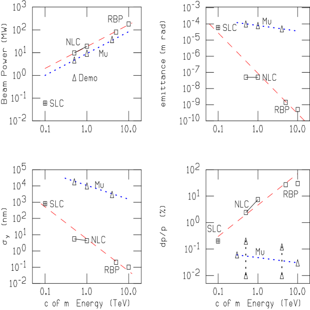
Figure 6.: Dependence of some sensitive parameters on linear collider energy, with comparison of same parameters for $\mu^{+}\mu^{-}$ colliders.

0.1.6 $\gamma-\gamma$ Colliders

A gamma-gamma collider[telnov] would use opposing electron linacs, as in a linear electron collider, but just prior to the collision point, laser beams would be Compton backscattered off the electrons to generate photon beams that would collide at the IP instead of the electrons. If suitable geometries are used, the mean photon-photon energy could be 80% or more of that of the electrons, with a luminosity about 1/10th.

If the electron beams, after they have backscattered the photons, are deflected, then backgrounds from beamstrahlung can be eliminated. The constraint on ${N/\sigma_{x}}$ in Eq.6 is thus removed and one might hope that higher luminosities would now be possible by raising $N$ and lowering $\sigma_{x}$. Unfortunately, to do this, one needs sources of larger number of electron bunches with smaller emittances, and one must find ways to accelerate and focus such beams without excessive emittance growth. Conventional damping rings will have difficulty doing this[mygamma]. Exotic electron sources would be needed, and methods using lasers to generate[palmerchen] or cool[telnovcool] the electrons and positrons are under consideration.

Thus, although gamma-gamma collisions can and should be made available at any future electron-positron linear collider, to add physics capability, they may not give higher luminosity for a given beam power.

0.1.7 $\mu^{+}\mu^{-}$ Colliders

There are two advantages of muons, as opposed to electrons, for a lepton collider.

• The synchrotron radiation, that forces high energy electron colliders to be linear, is (see Eq. 5) inversely proportional to the fourth power of mass: It is negligible in muon colliders with energy less than 10 TeV. Thus a muon collider, up to such energy, can be circular. In practice this means in can be smaller. The linacs for a 0.5 TeV NLC would be 20 km long. The ring for a muon collider of the same energy would be only about 1.2 km circumference.

• The luminosity of a muon collider is given by the same formula (Eq. 6) as given above for an electron positron collider, but there are two significant changes: 1) The classical radius $r_{o}$ is now that for the muon and is 200 times smaller; and 2) the number of collisions a bunch can make $n_{collisions}$ is no longer 1, but is now related to the average bending field in the muon collider ring, with

  $$n_{collisions}\ \approx\ 150\ B_{ave}$$

  With an average field of 6 Tesla, $n_{collisions}\approx 900$. Thus these two effects give muons an in principle luminosity advantage of more than $10^{5}$.

As a result of these gains, the required beam power, spot sizes, emittances and energy spread are far less in $\mu^{+}\mu^{-}$ colliders than in $e^{+}e^{-}$machines of the same energy. The comparison is made in Fig. 6 above.

But there are problems with the use of muons:

• Muons can be best be obtained from the decay of pions, made by higher energy protons impinging on a target. A high intensity proton source is thus required and very efficient capture and decay of these pions is essential.

• Because the muons are made with very large emittance, they must be cooled and this must be done very rapidly because of their short lifetime. Conventional synchrotron, electron, or stochastic cooling is too slow. Ionization cooling is the only clear possibility, but does not cool to very low emittances.

• Because of their short lifetime, conventional synchrotron acceleration would be too slow. Recirculating accelerators or pulsed synchrotrons must be used.

• Because they decay while stored in the collider, muons radiate the ring and detector with their decay products. Shielding is essential and backgrounds will certainly be significant.

These problems and their possible solutions will be discussed in more detail in the following chapters. Parameters will be given there of a 4 TeV center of mass collider, and of a 0.5 TeV demonstration machine.

0.1.8 Comparison of Machines

Length.

In Fig. 7, the effective physics energies (as defined by Eq. 4) of representative machines are plotted against their total tunnel lengths. We note:

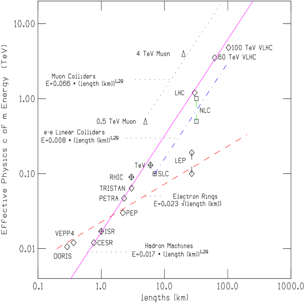
Figure 7.: Effective physics energies of colliders as a function of their total length.

• Hadrons Colliders: It is seen that the energies of machines rise with their size, but that this rise is faster than linear ($E_{\rm eff}\propto L^{1.3}$). This extra rise is a reflection of the steady increase in bending magnetic fields used as technologies and materials have become available.

• Circular Electron-Positron Colliders: The energies of these machines rise approximately as the square root of their size, as expected from the cost optimization discussed above.

• Linear Electron-Positron Colliders: The SLC is the only existing machine of this type and only one example of a proposed machine (the NLC) is plotted. The line drawn has the same slope as for the hadron machines and implies a similar rise in accelerating gradient, as technologies advance.

• Muon-Muon Colliders: Only the 4 TeV collider, discussed above, and the 0.5 TeV demonstration machine have been plotted. The line drawn has the same slope as for the hadron machines.

It is noted that the muon collider offers the greatest energy per unit length. This is also apparent in Fig. 8, in which the footprints of a number of proposed machines are given on the same scale. But does this mean it will give the greatest energy per unit of cost ?

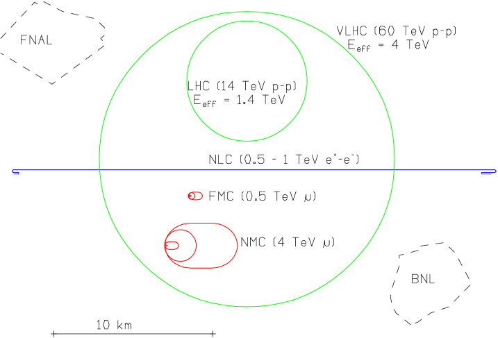
Figure 8.: Approximate sizes of some possible future colliders.

Cost.

Fig. 9 plots the cost of a sample of machines against their size. Before examining this plot, be warned: the numbers you will see will not be the ones you are familiar with. The published numbers for different projects use different accounting procedures and include different items in their costs. Not very exact corrections and escalation have been made to obtain estimates of the costs under fixed criteria: 1996 $’s, US accounting, no detectors or halls. The resulting numbers, as plotted, must be considered to have errors of at least $\pm$ 20%.

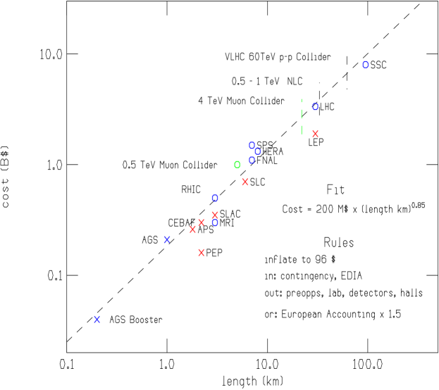
Figure 9.: Costs of some machines as a function of their total lengths.

The costs are seen to be surprisingly well represented by a straight line. Circular electron machines, as expected, lie significantly lower. The only plotted muon collider (the 0.5 TeV demonstration machine’s very preliminary cost estimate) lies above the line. But the clear indication is that length is, or at least has been, a good estimator of approximate cost. It is interesting to note that the fitted line indicates costs rising, not linearly, but as the 0.85 th power of length. This can be taken as a measure of economies of scale.

0.1.9 Conclusions

Our conclusions for this chapter, with the caveat that they are indeed only our opinions, are:

• The LHC is a well optimized and appropriate next step towards high effective physics energy.

• A Very Large Hadron Collider with energy greater than the SSC (e.g. 60 TeV c-of-m) and cost somewhat less than the SSC, may well be possible with the use of high T_c superconductors that may become available.

• A “Next Linear Collider” is the only clean way to complement the LHC with a lepton machine, and the only way to do so soon. But it appears that even a 0.5 TeV collider will be more expensive than the LHC, and it will be technically challenging: obtaining the design luminosity may not be easy.

• Extrapolating conventional rf $e^{+}e^{-}$linear colliders to energies above 1 or 2 TeV will be very difficult. Raising the rf frequency can reduce length and probably cost for a given energy, but obtaining luminosity increasing as the square of energy, as required, may not be feasible.

• Laser driven accelerators are becoming more realistic and can be expected to have a significantly lower cost per TeV. But the ratio of luminosity to wall power and the ability to preserve very small emittances, is likely to be significantly worse than for conventional rf driven machines. Colliders using such technologies are thus unlikely to achieve very high luminosities and are probably unsuitable for higher (above 2 TeV) energy physics research.

• A higher gradient superconducting Linac collider using Nb₃Sn or high T_c materials, if it becomes technically possible, could be the only way to attain the required luminosities in a higher energy $e^{+}e^{-}$collider.

• Gamma-gamma collisions can and should be obtained at any future electron-positron linear collider. They would add physics capability to such a machine, but, despite their freedom from the beamstrahlung constraint, may not achieve higher luminosity.

• A Muon Collider, being circular, could be far smaller than a conventional electron-positron collider of the same energy. Very preliminary estimates suggest that it would also be significantly cheaper. The ratio of luminosity to wall power for such machines, above 2 TeV, appears to be better than that for electron positron machines, and extrapolation to a center of mass energy of 4 TeV or above does not seem unreasonable. If research and development can show that it is practical, then a 0.5 TeV muon collider could be a useful complement to $e^{+}e^{-}$colliders, and, at higher energies (e.g. 4 TeV), could be a viable alternative.

0.2 PHYSICS CONSIDERATIONS

0.2.1 Introduction

The physics opportunities and possibilities of the muon collider have been well documented in the Feasibility Study[book] and by additional papers[ref100]. For most reactions the physics capabilities of $\mu^{+}\mu^{-}$ and $e^{+}e^{-}$ colliders with the same energy and luminosity are similar, so that the choice between them will depend mainly on the feasibility and cost of the accelerators. But for some reactions, the larger muon mass does provide some advantages:

• The suppression of synchrotron radiation induced by the opposite bunch (beamstrahlung) allows, in principle, the use of beams with very low momentum spread

• QED radiation is reduced by a factor of $[\ln(\sqrt{s}/m_{\mu})/\ln(\sqrt{s}/m_{e})]^{2}$, leading to smaller $\gamma\gamma$ backgrounds and a smaller effective beam energy spread.

• $s$-channel Higgs production is enhanced by a factor of $(m_{\mu}/m_{e})^{2}\approx 40000$.

• The suppression of synchrotron radiation, allowing acceleration and storage of muons in a ring, combined with the suppression of beamstrahlung, may allow the construction of $\mu^{+}\mu^{-}$ colliders at higher energy than $e^{+}e^{-}$machines.

The disadvantages are:

• Less polarization appears practical in a $\mu^{+}\mu^{-}$ collider than in an $e^{+}e^{-}$machine, and some luminosity loss is likely.

• The $\mu^{+}\mu^{-}$ machine will have considerably worse background and probably require a shielding cone, extending down to the vertex, that takes up a larger solid angle than that needed in an $e^{+}e^{-}$collider.

In the following sections we will give examples of physics for which there is a advantage in $\mu^{+}\mu^{-}$ . These examples are taken from the discussion in section II of the $\mu^{+}\mu^{-}$ Collider Feasibility Study [book]. For a discussion of the other physics, SUSY particle identification in particular, the reader is refered to the physics sections of the Next Linear Collider Zeroth Order Design Report (ZDR)[ZDR].

Precision Threshold Studies.

The high energy resolution and suppression of Initial State Radiation (ISR) in a $\mu^{+}\mu^{-}$ collider makes it particularly well suited to threshold studies. As an example, Fig. 10 shows the threshold curves for top quark production for both $\mu^{+}\mu^{-}$ and $e^{+}e^{-}$machines, with and without beam smearing. (An rms energy spread of 1 % is assumed for $e^{+}e^{-}$and 0.1 % for $\mu^{+}\mu^{-}$ ). The rms mass resolution $\Delta m_{t}$ obtained with $10\,{\rm fb}^{-1}$in a $\mu^{+}\mu^{-}$ Collider is estimated to be $\pm\,0.3\,{\rm GeV}.$ This can be compared with 4 GeV for the Tevatron, 2 GeV for the LHC, and 0.5 GeV for NLC.

Figure 10.: The threshold curves are shown for $\mu^{+}\mu^{-}$ and $e^{+}e^{-}$machines including ISR and with and without beam smearing. Beam smearing has only a small effect at a muon collider, whereas at an electron collider the threshold region is significantly smeared (An rms energy spread of $1\,\%$ is assumed for $e^{+}e^{-}$and $0.1\,\%$ for $\mu^{+}\mu^{-}$ ).

Studies of Standard Model, or SUSY Model Light, Higgs h.

The feature that has attracted most theoretical interest is the possibility of s-channel studies of Higgs production. This is possible with $\mu$’s, but not with e’s, due to the strong coupling of muons to the Higgs channel that is proportional to the mass of the lepton. If the Higgs sector is more complex than just a simple standard model (SM) Higgs, it will be necessary to measure the widths and quantum numbers of any newly discovered particles to ascertain the nature of those particles and the structure of the theory. In addition to the increased coupling strength of the muons, the beamstrahlung is much reduced for muons allowing much better definition of the beam energy.

Figure 11.: The (a) $h_{SM}$ signal and (b) background cross sections, $\epsilon\overline{\sigma}BF(X)$, for $X=b\overline{b}$, and useful (reconstructable, non-$4j$) $WW^{(\star)}$ and $ZZ^{(\star)}$ final states (including a channel-isolation efficiency of $\epsilon=0.5$) versus $m_{h_{SM}}$ for SM Higgs $s$-channel production. Also shown: (c) the corresponding luminosity required for a $S/\sqrt{B}=5$ standard deviations signal in each of the three channels. Results for $R=0.01\%$ and $R=0.06\%$ are given.

The cross sections for Higgs production with a $\mu^{+}\mu^{-}$ collider are substantial. Fig. 11 shows a) the Higgs signal, b) the background, and c) the luminosity required for a $5\,\sigma$ signal significance, for two different rms energy spreads of the muon beam: 0.01 % and 0.06 %. Signals are shown for three final states: $b\bar{b}$, WW^(∗) and ZZ^(∗) (reconstructable, non- 4 jet, with channel isolation efficiency $\epsilon$ = 0.5). It is seen that:

• For an rms energy resolution of 0.01 %, a luminosity of only 0.1  $fb^{-1}$ is required to yield a detectable signal for all $m_{h_{SM}}$ above the current LEP limit, except in the region of the Z peak, where 1 $fb^{-1}$ is required.

• For an rms energy resolution of 0.06 %, the luminosity required is 20- 30 times larger, indicating that the higher resolution is desirable even at significant loss of luminosity.

Figure 12.: Total width vs mass of the SM and MSSM Higgs bosons for $m_{t}=175~{}{\rm GeV}$. In the case of the MSSM, we have plotted results for $\tan\beta=2$ and 20, taking $m_{\widetilde{t}}=1~{}{\rm TeV}$ and including two-loop corrections.

Fig. 12 shows the total widths of standard model and MSSM Higgs. In the case of MSSM masses are plotted for the stop quark mass $m_{stop}$ = 1 TeV, tan $\beta$ = 2 and 20. Two loop corrections have been included, but no squark mixing or SUSY decay channels.

The standard model Higgs with mass below $m_{t}$ is seen to be very narrow. For 110 GeV it is $\approx$ 3 MeV. A Supersymmetric model Higgs would be wider, but might be only a little wider. It could be important to measure the width of a low mass Higgs to determine its character. It has been shown that a muon collider with an rms energy spread of 0.01 % could measure the width of a 110 GeV standard model Higgs to $\pm 1\,{\rm MeV}$ with only 2 inverse femtobarns. Only if the Higgs mass is close to that of the Z does it become difficult to make such a determination without a large amount of data (200 inverse femtobarns). This could be a very important measurement (that could not be done in any other way) since it would destinguish clearly the nature of the boson seen. Together with branching ratio measurements (also possible with a muon collider), it could even predict the mass of the other SUSY Higgs bosons: H and A.

Studies of SUSY Model Heavy Higgs Particles: H and A.

The H and A SUSY Higgs bosons are expected to be significantly heavier than the lightest h, and might have quite similar masses. If tan $\beta$ is small $(<3)$ then they can easily be identified at the LHC, but may not be identified there if tan $\beta$ is large. They could be searched for in an $e^{+}e^{-}$machine in $e^{+}e^{-}$$\rightarrow H,A$, (h,A, or h, A are depressed) but only up to about $m_{H,A}\approx\sqrt{s}/\sqrt{2}$ or even less. In a muon collider, on the other hand, they could, providing tan $\beta$ is large $(>3),$ be easily observed in the s-channel, up to masses equal to $\sqrt{s}$.

Studies of Non-SUSY Model Strong WW Interactions.

If SUSY does not exist and we are forced to a much higher mass scale to study the symmetry breaking process then a 4 TeV muon collider is a viable choice to study WW scattering as it becomes a strong reaction.

Fig. 0.2.1 shows the mass distribution for the $1\,{\rm TeV}$ Higgs signals and physics backgrounds from PYTHIA in a toy detector, which includes segmentation of $\Delta\eta=\Delta\phi=0.05$ and the angular coverage, $20^{\circ}<\theta<160^{\circ}$, assumed in the machine background calculations. Since the nominal luminosity is $1000\,{\rm fb}^{-1}$, there are $\mathrel{\hbox to0.0pt{\raise 2.20013pt\hbox{$>$}\hss}{\lower 2.20013pt\hbox{$\sim$}}}1000$ events per bin at the peak. The loss in signal from the $20^{\circ}$ cone is larger for this process than for $s$-channel processes but is still fairly small, as can be seen in Fig. 0.2.1. The dead cone has a larger effect on $\gamma\gamma\to WW$ and thus the accepted region has a better signal to background ratio.

Figure 13: Signals and physics backgrounds for a $1\,{\rm TeV}$ Higgs boson at a $\mu\mu$ collider, including the effect of a $20^{\circ}$ dead cone around the beamline. Figure 14: $WW\to WW$ signal and $\gamma\gamma\to WW$ background vs. the minimum angle, $\theta_{\rm min}$, of the $W$.

It would be desirable to separate the $WW$ and $ZZ$ final states in purely hadronic modes by reconstructing the masses. Whether this is possible or not will depend on the details of the calorimeter performance and the level of the machine backgrounds. If it is not, then one can use the $\sim 12\%$ of events in which one $Z\to ee$ or $\mu\mu$ to determine the $Z$ rate. Clearly there is a real challenge to try to measure the hadronic modes.

The background from $\gamma\gamma$ and $\gamma Z$ processes is smaller at a muon collider than at an electron collider but not negligible. Since the $p_{T}$ of the photons is usually very small while the $WW$ fusion process typically gives a $p_{T}$ of order $M_{W}$, these backgrounds can be reduced by making a cut $p_{T,WW}>50\,{\rm GeV}$. This cut keeps most of the signal while significantly reducing the physics background.

Summary.

For many reactions, SUSY particle discovery for example, an $e^{+}e^{-}$collider, with its higher polarization and lower background, would be preferable to a $\mu^{+}\mu^{-}$ machine of the same energy and luminosity. There are however specific reactions, s-channel Higgs production for example, where the $\mu^{+}\mu^{-}$ machine would have unique capabilities. Ideally both machines would be built and they would be complementary. Whether both machines could be built, at both moderate and multi TeV energies, and whether both could be afforded, remains to be determined.

There are several hardware questions that must be carefully studied. The first is the question of the luminosity available when the beam momentum spread is decreased. In addition there will have to be good control of the injected beam energy as there is not time to make large adjustments in the collider ring. Precision determination of the energy and energy spread will be mandatory: presumably by the study of spin precession. Finally, the question of luminosity vs. percent polarization needs additional study; unlike the electron collider, both beams can be polarized but as shown later in this report, but the luminosity decreases as the polarization increases.

0.3 MUON COLLIDER COMPONENTS

0.3.1 Introduction

The possibility of muon colliders was introduced by Skrinsky et al.[ref2] and Neuffer[ref3] and has been aggressively developed over the past two years in a series of meetings and workshops[ref4, ref5, ref6, ref7].

A collaboration, lead by BNL, FNAL and LBNL, with contributions from 18 institutions has been studying a 4 TeV, high luminosity scenario and presented a Feasibility Study[book] to the 1996 Snowmass Workshop. The basic parameters of this machine are shown schematically in Fig. 15 and given in Tb. 2. Fig. 16 shows a possible layout of such a machine.

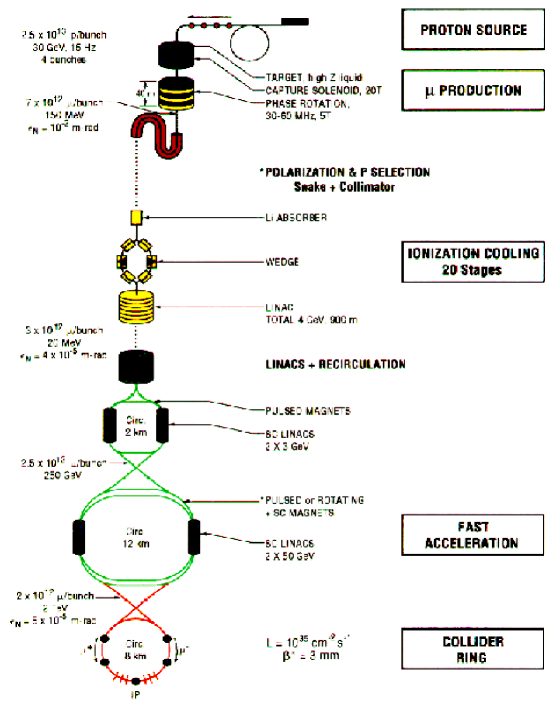
Figure 15.: Overview of a 4 TeV Muon Collider

Tb. 2 also gives the parameters of a 0.5 TeV demonstration machine based on the AGS as an injector. It is assumed that a demonstration version based on upgrades of the FERMILAB, or CERN machines would also be possible.

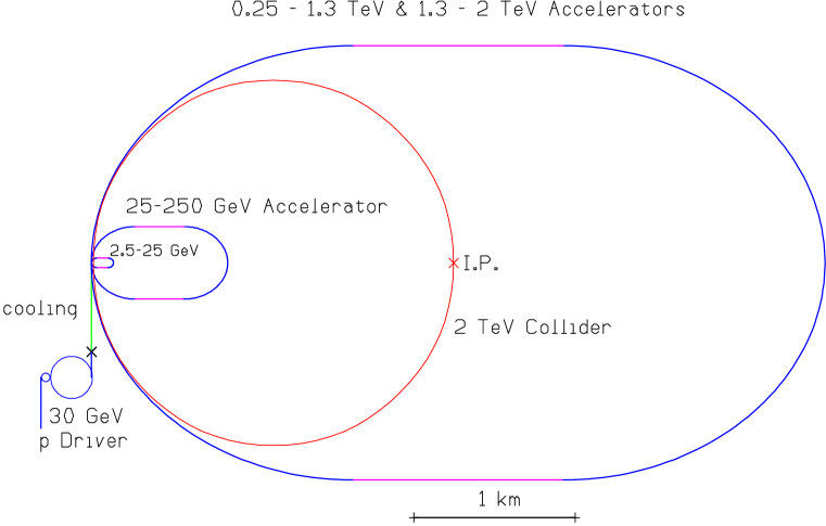
Figure 16.: Layout of the collider and accelerator rings.

Table 2.: Parameters of Collider Rings

c-of-m Energy	TeV	4	.5
Beam energy	TeV	2	.25
Beam $\gamma$		19,000	2,400
Repetition rate	Hz	15	2.5
Proton driver energy	GeV	30	24
Protons per pulse		$10^{14}$	$10^{14}$
Muons per bunch	$10^{12}$	2	4
Bunches of each sign		2	1
Beam power	MW	38	.7
Norm. rms emit. $\epsilon_{N}$	$\pi$ mm mrad	50	90
Bending Field	T	9	9
Circumference	Km	8	1.3
Ave. ring field $B$	T	6	5
Effective turns		900	800
$\beta^{*}$ at intersection	mm	3	8
rms I.P. beam size	$\mu m$	2.8	17
Chromaticity		2000-4000	40-80
$\beta_{\rm max}$	km	200-400	10-20
Luminosity	${\rm cm}^{-2}{\rm s}^{-1}$	$10^{35}$	$10^{33}$

The main components of the 4 TeV collider would be:

• A proton source with KAON like parameters (30 GeV, $10^{14}$ protons per pulse, at 15 Hz).

• A liquid metal target surrounded by a 20 T hybrid solenoid to make and capture pions.

• A 5 T solenoidal channel within a sequence of rf cavities to allow the pions to decay into muons and, at the same time, decelerate the fast ones that come first, while accelerating the lower momentum ones that come later. Muons from pions in the 100-500 MeV range emerge in a 6 m long bunch at 150 $\pm$ 30 MeV.

• A solenoidal snake and collimator to select the momentum, and thus polarization, of the muons.

• A sequence of 20 ionization cooling stages, each consisting of: a) energy loss material in a strong focusing environment for transverse cooling; b) linac reacceleration and c) lithium wedges in a dispersive environment for cooling in momentum space.

• A linac and/or recirculating linac pre-accelerator, followed by a sequence of pulsed field synchrotron accelerators using superconducting linacs for rf.

• An isochronous collider ring with locally corrected low beta ($\beta$=3 mm) insertion.

0.3.2 Proton Driver

The specifications of the proton drivers are given in Tb 3. In the 4 TeV example, it is a high-intensity (4 bunch, $2.5\times 10^{13}$ protons per pulse) 30 GeV proton synchrotron. The preferred cycling rate would be 15 Hz, but for a demonstration machine using the AGS[ref8], the repetition rate would be limited to 2.5 Hz and the energy to $24\,$GeV. For the lower energy machine, 2 final bunches are employed (one to make $\mu^{-}$’s and the other to make $\mu^{+}$’s). For the high energy collider, four are used (two $\mu$ bunches of each sign).

Table 3.: Proton Driver Specifications

		4 TeV	.5 TeV Demo
Proton energy	GeV	30	24
Repetition rate	Hz	15	2.5
Protons per bunch	$10^{13}$	2.5	5
Bunches		4	2
Long. phase space/bunch	eV s	5	10
Final rms bunch length	ns	1	1

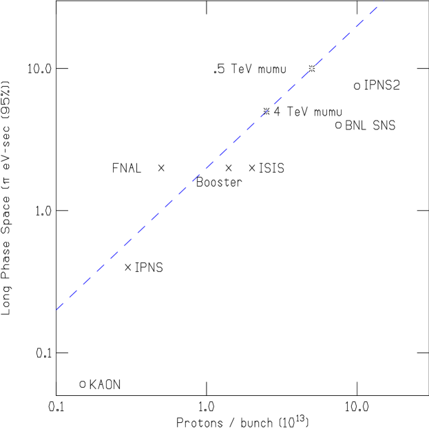
Figure 17.: Longitudinal Phase Space of Bunches vs. number of Protons; x’s indicate existing machines, circles proposed machines, and stars the values used here

In order to reduce the cost of the muon phase rotation section, minimize the final muon longitudinal phase space and maximize the achievable polarization,, it appears that the final proton bunch length should be of the order of 1 ns. Is this practical ?

There appears to be a relationship between the number of protons in a bunch and the longitudinal phase space of that bunch that can be maintained stability in a circular machine. Fig. 17 shows values obtained and those planned in a number of machines. The conservative assumption is that phase space densities will be similar to those already achieved: around 2 eV seconds per $10^{13}$ protons, as indicated by the line in Fig. 17. The required bunches of $2.5\ 10^{13}$ protons would thus be expected to have a phase space of $5\,{\rm eVs}$ (at 95%) = $6\pi\,\sigma_{t}\sigma_{E}\ {\rm eVs}$ rms. A 1 ns rms bunch at 30 GeV with this phase space will have an rms momentum spread of $0.8\,\%,$ ($2\,\%$ at 95%), and the space charge tune shift just before extraction would be $\approx 0.5.$ Provided the rotation can be performed rapidly enough, this should not be a problem. For the 0.5 TeV machine the bunch intensity, and thus area, would be double, leading to a final spread of 1.6 % rms (4 % at 95 %).

An attractive technique[ref11] for bunch compression would be to generate a large momentum spread with modest rf at a final energy close to transition. Pulsed quads would then be employed to move the operating point away from transition, resulting in rapid compression.

Earlier studies had suggested that the driver could be a 10 GeV machine with the same charge per fill, but a repetition rate of $30\,$Hz. This specification was almost identical to that studied[ref9] at ANL for a spallation neutron source. Studies at FNAL[ref10] have further established that such a specification is reasonable. But if 10 GeV protons are used, then approximately twice as many protons per bunch are required for the same pion production: $5\times 10^{13}$ per bunch for the 4 TeV case, $1\times 10^{14}$ per bunch for the 0.5 TeV case; the phase space of the bunches would be expected to be twice as big and the resulting % momentum spread for the 1 ns bunch 6 times as large: i.e. 12 % (at 95%) which may be hard to achieve. For the 0.5 TeV specification, this rises to 24 %: clearly unreasonable.

0.3.3 Target and Pion Capture

Pion Production.

Predictions of the nuclear Monte-Carlo program ARC[ref12] suggest that $\pi$ production is maximized by the use of heavy target materials, and that the production is peaked at a relatively low pion energy ($\approx 100\,$MeV), substantially independent of the initial proton energy. Fig.18 shows the forward $\pi^{+}$ production as a function of proton energy and target material; the $\pi^{-}$ distributions are similar.

Figure 18.: ARC forward $\pi^{+}$ production vs. proton energy and target material.

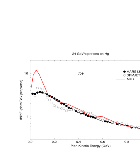
Figure 19.: $\pi^{+}$ energy distribution for $24\,$GeV protons on Hg.

Other programs[ref13],[ref14] do not predict such a large low energy peak,(see for instance Fig. 19) and there is currently very little data to indicate which is right. An experiment (E910)[ref15a][ref15b], currently running at the AGS, should decide this question, and thus settle at which energy the capture should be optimized.

Target.

For a low repetition rate the target could probably be made of Cu, approximately 24 cm long by 2 cm diameter. A study[ref15] indicates that, with a 3 mm rms beam, the single pulse instantaneous temperature rise is acceptable, but, if cooling is only supplied from the outside, the equilibrium temperature, at our required repetition rate, would be excessive. Some method must be provided to give cooling within the target volume. For instance, the target could be made of a stack of relatively thin copper disks, with water cooling between them. A graphite target could be used, but with significant loss of pion production, or a liquid metal target. Liquid lead and gallium are under consideration. In order to avoid shock damage to a container, the liquid could be in the form of a jet.

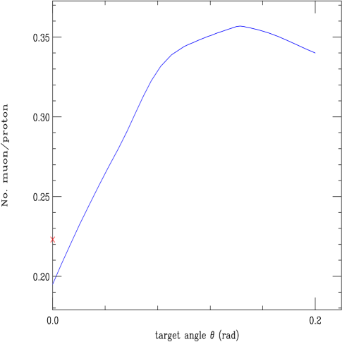
Figure 20.: The muon to proton ratio as a function of the skew angle for a target whose length and transverse position has been reoptimized for the skew case. The single x indicates the production ratio at zero angle with the original optimization.

It appears that for maximum muon yield, the target (and incoming beam) should be at an angle to the axis of the solenoid and outgoing beam. The introduction of such an angle reduces the loss of pions when they reenter the target after being focused by the solenoid. A Monte Carlo simulation[bob&juan] gave a muon production increase of 60 % with at an angle 150 milliradians. The simulation assumed a copper target (interaction length 15 cm), ARC[ref12] pion production spectra, a fixed pion absorption cross section, no secondary pion production, a 1 cm target radius, and the capture solenoid, decay channel, phase rotation and bunch defining cuts described below. Fig. 20 shows the final muon to proton ratio as a function of the skew angle for a target whose length (45 cm) and transverse position (front end displaced - 1.5 cm from the axis) had been reoptimized for the skew case. The single X indicates the production ratio at zero angle with the original optimization (target length 30 cm, on axis). One notes that the reoptimized target length is 3 interaction lengths long, and thus absorbs essentially all of the initial protons.

Capture.

Several capture methods were studied[myoldcapture]. Pulsed horns were effective at the capture of very high energy pions. Multiple lithium lenses were more effective at lower pion energies, but neither was as effective as a high field solenoid at the 100 MeV peak of the pion spectrum. Initially, a $15\,{\rm cm}$ diameter, $28\,T$ field was considered. Such a magnet could probably be built using superconducting outer coils and a Bitter, or other immersed sheet conductor inner coil, but such an immersed coil would probably have limited life[ref16]. A 15 cm diameter, $20\,T$ solenoid could use a more conventional hollow conductor inner coil and was thus chosen despite the loss of 24 % pion capture (see Fig. 21)

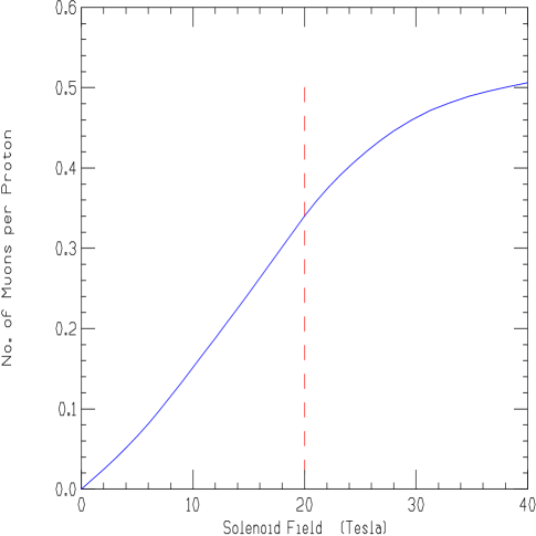
Figure 21.: The muon to proton ratio as a function of capture solenoid field

A preliminary design[ref16] (see Fig. 22) has an inner Bitter magnet with an inside diameter of 24 cm (space is allowed for a 4 cm heavy metal shield inside the coil) and an outside diameter of 60 cm; it provides half (10T) of the total field, and would consume approximately 8 MW. The superconducting magnet has a set of three coils, all with inside diameters of 70 cm and is designed to give 10 T at the target and provide the required tapered field to match into the periodic superconducting solenoidal decay channel ($5\,$T and radius $=15\,$cm). A similar design has been made at LBL[mikegreens].

A new design[weggelnew] using a hollow conductor insert is now in progress. The resistive coil would give 6 T and consume 4 MW. The superconducting coils will supply 14 T.

Figure 22.: Schematic of a hybrid magnet solenoid system for $\pi$ capture and matching.

Monte Carlo studies indicate a yield of 0.4–0.6 muons, of each sign, per initial proton, captured in the decay channel. Surprisingly, this conclusion seems relatively independent of whether the system is optimized for energies of 50 to 500 MeV (using ARC), or 200 to 2000 MeV (using MARS).

Use of Both Signs.

Protons on the target produce pions of both signs, and a solenoid will capture both, but the required subsequent phase rotation rf systems will have opposite effects on each. One solution is to break the proton bunch into two, aim them on the same target one after the other, and adjust the rf phases such as to act correctly on one sign of the first bunch and on the other sign of the second. This is the solution assumed in the parameters of this paper.

A second possibility would be to separate the charges into two channels, delay the particles of one charge by introducing a chicane in one of the channels, and then recombine the two channels so that the particles of the two charges are in line, but separated longitudinally (i.e. box cared). Both charges can now be phase rotated by a single linac with appropriate phases of rf.

A third solution is to separate the pions of each charge prior to the use of rf, and feed the beams of each charge into different channels.

In either of the latter two solutions, there is a problem in separating the beams. After the target, and prior to the use of any rf or cooling, the beams have very large emittances and energy spread. Conventional charge separation using a dipole is not practical. But if a solenoidal channel is bent, then the particles trapped within that channel will drift[ref15],[drift], in a direction perpendicular to the bend (this effect is discussed in more detail in the section on Options below). With our parameters this drift is dominated by a term (curvature drift) that is linear with the forward momentum of the particles, and has a direction that depends on the sign of the charges. If sufficient bend is employed[ref15], the two charges could be separated by a septum and captured into two separate channels. When these separate channels are bent back to the same forward direction, the momentum dispersion is separately removed in each new channel.

Although this idea is very attractive, it has some problems:

• If the initial beam has a radius r=$0.15\,$m, and if the momentum range to be accepted is $F={p_{{\rm max}}\over p_{{\rm min}}}=3,$ then the required height of the solenoid just prior to separation is 2(1+F)r=$1.2\,$m. Use of a lesser height will result in particle loss. Typically, the reduction in yield for a curved solenoid compared to a straight solenoid is about $25\,\%$ (due to the loss of very low and very high momentum pions), but this must be weighed against the fact that both charge signs are captured for each proton on target.

• The system of bend, separation, and return bend will require significant length and must occur prior to the start of phase rotation (see below). Unfortunately, it appears that the cost of the phase rotation rf is strongly dependent on keeping this distance as short as possible.

Clearly, compromises will be involved, and more study of this concept is required.

0.3.4 Phase Rotation Linac

The pions, and the muons into which they decay, have an energy spread from about 0 - 500 MeV, with an rms/mean of $\approx 100\%$, and peak at about 100 MeV. It would be difficult to handle such a wide spread in any subsequent system. A linac is thus introduced along the decay channel, with frequencies and phases chosen to deaccelerate the fast particles and accelerate the slow ones; i.e. to phase rotate the muon bunch. Tb. 4 gives an example of parameters of such a linac. It is seen that the lowest frequency is 30 MHz, a low but not impossible frequency for a conventional structure.

Table 4.: Parameters of Phase Rotation Linacs

Linac	Length	Frequency	Gradient
	m	MHz	MeV/m
1	3	60	5
2	29	30	4
3	5	60	4
4	5	37	4

A design of a reentrant 30 MHz cavity is shown in Fig.23. Its parameters are given in Tb.5.

Table 5.: Parameters of 30 MHz rf Cavity

Cavity Radius	cm	101
Cavity Length	cm	120
Beam Pipe Radius	cm	15
Accelerating Gap	cm	24
Q		18200
Average Acceleration Gradient	MV/m	3
Peak rf Power	MW	6.3
Average Power (15 Hz)	KW	18.2
Stored Energy	J	609

It has a diameter of approximately 2 m, only about one third of that of a conventional pill-box cavity. To keep its cost down, it would be made of aluminum. Multipactoring would probably be suppressed by stray fields from the 5 T focusing coils, but could also be controlled by an internal coating of titanium nitride.

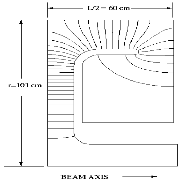
Figure 23.: 30 MHz cavity for use in phase rotation and early stages of cooling.

Figs. 24 and 25 show the energy vs. c t at the end of the decay channel with and without phase rotation. Note that the c t scales are very different: the rotation both compacts the energy spread and limits the growth of the bunch length.

Figure 24.: Energy vs. ct of Muons at End of Decay Channel without Phase Rotation.

After this phase rotation, a bunch can be selected with mean energy 150 MeV, rms bunch length $1.7\,$m, and rms momentum spread $20\,$% ($95\,$%, $\epsilon_{\rm L}=3.2\,{\rm eVs}$). The number of muons per initial proton in this selected bunch is 0.35, about half the total number of pions initially captured. As noted above, since the linacs cannot phase rotate both signs in the same bunch, we need two bunches: the phases are set to rotate the $\mu^{+}$’s of one bunch and the $\mu^{-}$’s of the other. Prior to cooling, the bunch is accelerated to 300 MeV, in order to reduce the momentum spread to $10\,\%.$

Figure 25.: Energy vs. ct of Muons at End of Decay Channel with Phase Rotation.

0.3.5 Cooling

For a collider, the phase-space volume must be reduced within the $\mu$ lifetime. Cooling by synchrotron radiation, conventional stochastic cooling and conventional electron cooling are all too slow. Optical stochastic cooling[ref11a], electron cooling in a plasma discharge[ref12a] and cooling in a crystal lattice[ref13a] are being studied, but appear very difficult. Ionization cooling[ref14a] of muons seems relatively straightforward.

Ionization Cooling Theory.

In ionization cooling, the beam loses both transverse and longitudinal momentum as it passes through a material medium. Subsequently, the longitudinal momentum can be restored by coherent reacceleration, leaving a net loss of transverse momentum. Ionization cooling is not practical for protons and electrons because of nuclear interactions (p’s) and bremsstrahlung (e’s), but is practical for $\mu$’s because of their low nuclear cross section and relatively low bremsstrahlung.

The approximate equation for transverse cooling (with energies in GeV) is:

$$\frac{d\epsilon_{n}}{ds}\ \approx\ -\frac{dE_{\mu}}{ds}\ \frac{\epsilon_{n}}{E_{\mu}}\ +\ \frac{\beta_{\perp}(0.014)^{2}}{2\ E_{\mu}m_{\mu}\ L_{R}},$$ (11)

where $\epsilon_{n}$ is the normalized emittance, $\beta_{\perp}$ is the betatron function at the absorber, $dE_{\mu}/ds$ is the energy loss, and $L_{R}$ is the radiation length of the material. The first term in this equation is the coherent cooling term, and the second is the heating due to multiple scattering. This heating term is minimized if $\beta_{\perp}$ is small (strong-focusing) and $L_{R}$ is large (a low-Z absorber). From Eq. 11 we find a limit to transverse cooling, which occurs when heating due to multiple scattering balances cooling due to energy loss. The limits are $\epsilon_{n}\approx\ 0.6\ 10^{-2}\ \beta_{\perp}$ for Li, and $\epsilon_{n}\approx\ 0.8\ 10^{-2}\ \beta_{\perp}$ for Be.

The equation for energy spread (longitudinal emittance) is:

$${\frac{d(\Delta E)^{2}}{ds}}\ \approx\ -2\ {\frac{d\left({\frac{dE_{\mu}}{ds}}\right)}{dE_{\mu}}}\ <(\Delta E_{\mu})^{2}>\ +\ {\frac{d(\Delta E_{\mu})^{2}_{{\rm straggling}}}{ds}}$$ (12)

where the first term is the cooling (or heating) due to energy loss, and the second term is the heating due to straggling.

Cooling requires that ${d(dE_{\mu}/ds)\over dE_{\mu}}>0.$ But at energies below about 200 MeV, the energy loss function for muons, $dE_{\mu}/ds$, is decreasing with energy and there is thus heating of the beam. Above 400 MeV the energy loss function increases gently, giving some cooling, but not sufficient for our application.

Energy spread can also be reduced by artificially increasing ${d(dE_{\mu}/ds)\over dE_{\mu}}$ by placing a transverse variation in absorber density or thickness at a location where position is energy dependent, i.e. where there is dispersion. The use of such wedges can reduce energy spread, but it simultaneously increases transverse emittance in the direction of the dispersion. Six dimensional phase space is not reduced, but it does allow the exchange of emittance between the longitudinal and transverse directions.

In the long-path-length Gaussian-distribution limit, the heating term (energy straggling) is given by[ref15c]

$$\frac{d(\Delta E_{\mu})^{2}_{{\rm straggling}}}{ds}\ =\ 4\pi\ (r_{e}m_{e}c^{2})^{2}\ N_{o}\ \frac{Z}{A}\ \rho\gamma^{2}\left(1-\frac{\beta^{2}}{2}\right),$$ (13)

where $N_{o}$ is Avogadro’s number and $\rho$ is the density. Since the energy straggling increases as $\gamma^{2}$, and the cooling system size scales as $\gamma$, cooling at low energies is desired.

0.3.6 Low $\beta_{\perp}$ Lattices for Cooling

We have seen from the above that for a low equilibrium emittance we require energy loss in a strong focusing (low $\beta_{\perp}$) region. Three sources of strong focusing have been studied:

Solenoid.

The simplest solution would appear to be the use of a long high field solenoid in which both acceleration and energy loss material could be contained. There is, however, a problem: when particles enter a solenoid other than on the axis, they are given angular momentum by the radial field components that they must pass. This initial angular momentum is proportional to the solenoid field strength, and to the particles’ radius. In the absence of material, this extra angular momentum is maintained proportional to the tracks’ radius as they pass along the solenoid until they are exactly corrected by the radial fields at the exit. But if material is introduced, all transverse momenta are “cooled”, including the extra angular momentum given by these radial fields. When the cooled particles now leave the solenoid, then the end fields overcorrect them, leaving the particles with a finite added angular momentum. In practice, this angular momentum is equivalent to a significant heating term that limits the maximum emittance reduction to a quite small factor. The problem can only be averted if the direction of the solenoid field is periodically reversed.

Alternating Solenoid (FOFO) Lattice.

An interesting case of such periodic solenoid field reversals is a lattice with rapid reversal that, for example, might approximate sinusoidal variations. We describe such a lattice as FOFO (focus focus) in analogy with quadrupole lattices that are FODO (focus defocus). Not only do such lattices avoid the angular momentum problems of a long solenoid, but they can, if the phase advance per cell approaches $\pi$, provide $\beta_{\perp}$’s at the zero field points, that are less than the same field would provide in the long solenoid case.

But as noted above, for cooling to be effective, the ratio of emittance to $\beta_{\perp}$ must remain above a given value. This implies that the angular amplitude of the particles has to be relatively large (typically greater than 0.1 radians rms). When tracking of such distributions was performed on realistic lattices three apparent problems were observed:

1. Particles entering with large amplitude (radius or angle) were found[neufferandy] to be lost or reflected by the fringe fields of the lenses. The basic problem is that there are strong non-linear effects that focus the large angle particles more strongly than those at small angles (this is known as a second order tune shift). The stronger focus causes an increase in the phase advance per cell resulting in resonant behavior, emittance growth and particle loss.

2. A bunch, even when monoenergetic, passing along such a lattice would be seen[fernow] to rapidly grow in length because the larger amplitude particles, traveling longer orbits, would fall behind the small amplitude ones.

3. With material present, the energy spread of a bunch grew because the high amplitude particles were passing through more material than the low amplitude ones.

Surprisingly however, none of these turns out to be a real problem. If the particles are matched, as they must be, into rf buckets, then all particles at the centers of these buckets must be traveling with the same average forward velocity. If this were not so then they would be arriving at the next rf cavity with different phases and would not be at the center of the bucket. It follows that large amplitude particles (whose trajectories are longer) must have higher momenta than those with lower amplitude. The generation of this correlation is part of the matching requirement, and would be naturally generated if an adiabatic application of FOFO strength were introduced. It could also be generated by a suitable gradation of the average radial absorber density.

Since higher amplitude particles will thus have higher momenta, they will, as a result, be less strongly focused: an effect of the opposite sign to the second order tune shift natural to the lattice. Can the effects cancel ? In practice they are found to cancel almost exactly at a specific momentum: close to 100 MeV/c for a continuous sinusoidal FOFO lattice (the exact momentum will depend on the lattice).

A second, but only partial, cancelation also occurs: the higher amplitude, and now higher momentum, particles lose less energy in the absorber because of the natural energy dependence of the energy loss. This difference of energy loss, at 100 MeV/c, actually overcorrects the difference in energy loss from the difference in trajectories in the material. But this too is no problem. The natural bucket center for large amplitude particles will be displaced not only up in energy, but also over in phase, so as to be in a different accelerating field, and thus maintain their energy. Again, this would occur naturally if the lattice is introduced adiabatically and can also be generated by a combination of radially graded absorbers and drifts. Particles of differing momentum or phase will, as in normal synchrotron oscillation, gyrate about their bucket centers, but now each amplitude has a different center.

Using particles so matched, a simulation using fully Maxwellian sinusoidal field has been shown to give continuous transverse cooling without significant particle loss (see Fig. 26). In this simulation, the axial field has been gradually increased, and its period decreased, so as to maintain a constant rms angular spread as the emittance falls. The peak rf accelerating fields were 10 MeV/m, their frequency 750 MHz, the absorbing material was lithium, placed at the zero magnetic field positions, with lengths such that they occupied 5 % of the length. The mean momentum was 110 MeV/c, and rms width 2 %. 500 particles were tracked; none were lost.

Figure 26.: Cooling in a FOFO Lattice: (a) rms radius; (b) normalized emittance; and (c) axial magnetic fields; all plotted vs axial length.

Lithium Rods.

The third method of providing strong focusing and energy loss is to pass the particles along a current carrying lithium rod (a long lithium lens). The rod serves simultaneously to maintain the low $\beta_{\perp}$, and attenuate the beam momenta. Similar lithium rods, with surface fields of $10\,$T , were developed at Novosibirsk[ref16a] and have been used as focusing elements at FNAL[fermilab_li] and CERN[cern_li]. At the repetition rates required here, cooling of a solid rod will not be possible, and circulating liquid columns will have to be used. A small lens using such liquid cooling has also been tested at Novosibirsk. It is also hoped[20Tli] that because of the higher compressibility of the liquid, surface field up to 20 T may be possible.

Lithium lenses will permit smaller $\beta_{\perp}$ and therefore cooling to lower emittances than in a practicable FOFO lattice, and such rods are thus preferred for the final cooling stages. But they are pulsed devices and consequently they are likely to have significant life time problems, and are thus not preferred for the earlier stages where they are not absolutely needed.

Such rods do not avoid the second order tune shift complications discussed above for the FOFO lattices. The rods must be alternated with acceleration sections and thus the particles must periodically be focused into and out of the rods. All three of the nonlinear effects enumerated above will be encountered. It is reasonable to believe that they can be controlled by the same mechanisms, but a full simulation of this has not yet been done.

Emittance Exchange Wedges.

Emittance exchange in wedges to reduce the longitudinal emittance has been modeled with Monte Carlo calculations and works as theoretically predicted. But the lattices needed to generate the required dispersions and focus the particles onto the wedges have yet to be designed. The nonlinear complications discussed above will again have to be studied and corrected.

Emittance exchange in a bent current carrying rod has also been studied, both for a rod of uniform density[fredmills] (in which the longer path length on the outside of the helix plays the role of a wedge; and where the average rod density is made greater on the outside of the bends by the use of wedges of a more dense material[sasha].

Reverse Emittance Exchange.

At the end of a sequence of a cooling elements, the transverse emittance may not be as low as required, while the longitudinal emittance, has been cooled to a value less than is required. The additional reduction of transverse emittance can then be obtained by a reverse exchange of transverse and longitudinal phase-spaces. This can be done in one of several ways:

1. by the use of wedged absorbers in dispersive regions between solenoid elements.

2. by the use of septa that subdivide the transverse beam size, acceleration that shifts the energies of the parts, and bending to recombine the parts[sasha].

3. by the use of lithium lenses at very low energy: at very low energies the $\beta_{\perp}$’s, and thus equilibrium emittances, can be made arbitrarily low; but the energy spread is blown up by the steep rise in dE/dx. If this blow up of dE/dx is left uncorrected, then the effect can be close to an emittance exchange.

0.3.7 Model Cooling System

We require a reduction of the normalized transverse emittance by almost three orders of magnitude (from $1\times 10^{-2}$ to $5\times 10^{-5}\,$m-rad), and a reduction of the longitudinal emittance by one order of magnitude.

A model example has been generated that uses no recirculating loops, and it is assumed for simplicity that the beams of each charge are cooled in separate channels (it may be possible to design a system with both charges in the same channel). The cooling is obtained in a series of cooling stages. In the early stages, they each have two components:

1. FOFO lattice consisting of spaced axial solenoids with alternating field directions and lithium hydride absorbers placed at the centers of the spaces between them where the $\beta_{\perp}$’s are minimum. RF cavities are introduced between the absorbers along the entire length of the lattice.

2. A lattice consisting of more widely separated alternating solenoids, and bending magnets between them to generate dispersion. At the location of maximum dispersion, wedges of lithium hydride are introduced to interchange longitudinal and transverse emittance.

In the last stages, reverse emittance exchange is achieved using current carrying lithium rods. The energy is allowed to fall to 15 MeV, thus increasing the focussing strength and lowering $\beta_{\perp}$.

The design is based on analytic calculations. The phase advance in each cell of the FOFO lattice is made as close to $\pi$ as possible in order to minimize the $\beta_{\perp}$’s at the location of the absorber. The following effects are included: space charge transverse defocusing and longitudinal space charge forces; a $3\,\sigma$ fluctuation of momentum and $3\,\sigma$ fluctuations in amplitude.

The emittances, transverse and longitudinal, as a function of stage number, are shown in Fig.27, together with the beam energy. In the first 15 stages, relatively strong wedges are used to rapidly reduce the longitudinal emittance, while the transverse emittance is reduced relatively slowly. The objective is to reduce the bunch length, thus allowing the use of higher frequency and higher gradient rf in the reacceleration linacs. In the next 10 stages, the emittances are reduced close to their asymptotic limits. In the final three stages, lithium rods are used to produce an effective emittance exchange, as described above.

Individual components of the lattices have been defined, but a complete lattice has not yet been specified, and no complete Monte Carlo study of its performance has yet been performed. Wake fields, resistive wall effects, second order rf effects and some higher order focus effects are not yet included in this design of the system.

The total length of the system is 750 m, and the total acceleration used is 4.7 GeV. The fraction of muons that have not decayed and are available for acceleration is calculated to be $55\,$%.

It would be desirable, though not necessarily practical, to economize on linac sections by forming groups of stages into recirculating loops.

Figure 27.: $\epsilon_{\perp}$, ${\epsilon_{L}\,c\over\left<{\rm E}_{\mu}\right>}$ and E_μ [GeV] vs. stage number in the cooling sequence.

0.3.8 Acceleration

Following cooling and initial bunch compression the beams must be rapidly accelerated to full energy (2 TeV, or 250 GeV). A sequence of linacs would work, but would be expensive. Conventional synchrotrons cannot be used because the muons would decay before reaching the required energy. The conservative solution is to use a sequence of recirculating accelerators (similar to that used at CEBAF). A more economical solution would be to use fast rise time pulsed magnets in synchrotrons, or synchrotrons with rapidly rotating permanent magnets interspersed with high field fixed magnets.

Recirculating Acceleration.

Tb. 6 gives an example of a possible sequence of recirculating accelerators. After initial linacs, there are two conventional rf recirculating accelerators taking the muons up to 75 GeV, then two superconducting recirculators going up to 2000 GeV.

Table 6.: Parameters of Recirculating Accelerators

		Linac	#1	#2	#3	#4
initial energy	GeV	0.20	1	8	75	250
final energy	GeV	1	8	75	250	2000
nloop		1	12	18	18	18
freq.	MHz	100	100	400	1300	2000
linac V	GV	0.80	0.58	3.72	9.72	97.20
grad		5	5	10	15	20
dp/p initial	%	12	2.70	1.50	1	1
dp/p final	%	2.70	1.50	1	1	0.20
$\sigma_{z}$ initial	mm	341	333	82.52	14.52	4.79
$\sigma_{z}$ final	mm	303	75.02	13.20	4.36	3.00
$\eta$	%	1.04	0.95	1.74	3.64	4.01
$N_{\mu}$	$10^{12}$	2.59	2.35	2.17	2.09	2
$\tau_{fill}$	$\mu$s	87.17	87.17	10.90	s.c.	s.c.
beam t	$\mu$s	0.58	6.55	49.25	103	805
decay survival		0.94	0.91	0.92	0.97	0.95
linac len	km	0.16	0.12	0.37	0.65	4.86
arc len	km	0.01	0.05	0.45	1.07	8.55
tot circ	km	0.17	0.16	0.82	1.72	13.41
phase slip	deg	0	38.37	7.69	0.50	0.51

Criteria that must be considered in picking the parameters of such accelerators are:

• The wavelengths of rf should be chosen to limit the loading, $\eta$, (it is restricted to below 4 % in this example) to avoid excessive longitudinal wakefields and the resultant emittance growth.

• The wavelength should also be sufficiently large compared to the bunch length to avoid excessive second order effects (in this example: 10 times).

• For power efficiency, the cavity fill time should be long compared to the acceleration time. When conventional cavities cannot satisfy this condition, superconducting cavities are specified.

• In order to minimize muon decay during acceleration (in this example 73% of the muons are accelerated without decay), the number of recirculations at each stage should be kept low, and the rf acceleration voltage correspondingly high. For minimum cost, the number of recirculations appears to be of the order of 18. In order to avoid a large number of separate magnets, multiple aperture magnets can be designed (see Fig.28).

Note that the linacs see two bunches of opposite signs, passing through in opposite directions. In the final accelerator in the 2 TeV case, each bunch passes through the linac 18 times. The total loading is then $4\times 18\times\eta=288\%.$ With this loading, assuming 60% klystron efficiencies and reasonable cryogenic loads, one could probably achieve 35% wall to beam power efficiency, giving a wall power consumption for the rf in this ring of 108 MW.

A recent study[neufferacc] tracked particles through a similar sequence of recirculating accelerators and found a dilution of longitudinal phase space of the order of 15% and negligible particle loss.

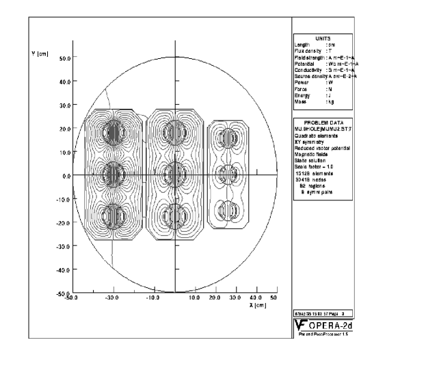
Figure 28.: A cross section of a 9 aperture sc magnet.

Pulsed Magnet Acceleration.

An alternative to recirculating accelerators for stages #2 and #3 would be to use pulsed magnet synchrotrons with rf systems consisting of significant lengths of superconducting linac.

The cross section of a pulsed magnet for this purpose is shown in Fig. 29. If desired, the number of recirculations could be higher in this case, and the needed rf voltage correspondingly lower, but the loss of particles from decay would be somewhat more. The cost for a pulsed magnet system appears to be significantly less than that of a multi-hole recirculating magnet system, and the power consumption is moderate for energies up to 250 GeV. Unfortunately, the power consumption is impractical at energies above 500 GeV.

Figure 29.: Cross section of pulsed magnet for use in the acceleration to 250 GeV.

Pulsed and Superconducting Hybrid.

For the final acceleration to 2 TeV in the high energy machine, the power consumed by a ring using only pulsed magnets would be excessive, but a hybrid ring with alternating pulsed warm magnets and fixed superconducting magnets[rotating][summers2] should be a good alternative.

Tb. 7 gives an example of a possible sequence of such accelerators. Fig. 16 used a layout of this sequence. The first two rings use pulsed cosine theta magnets with peak fields of $3\,$T and $4\,$T. Then follow two hybrid magnet rings with $8\,$T fixed magnets alternating with $\pm 2\,$T iron yoke pulsed magnets. The latter two rings share the same tunnel, and might share the same linac too. The survival from decay after all four rings is $67\,\%.$ Phase space dilution should be similar to that determined for the recirculating accelerator design above.

Table 7.: Parameters of Pulsed Accelerators

	Ring	1	2	3	4
$E_{init}$	(GeV)	2.5	25	250	1350
$E_{final}$	(GeV)	25	250	1350	2000
fract pulsed	%	100	100	73	44
$B_{pulsed}$	(T)	3	4	$\pm 2$	$\pm 2$
Acc/turn	(GeV)	1	7	40	40
Acc Grad	(MV/m)	10	12	20	20
RF Freq	(MHz)	100	400	1300	1300
circumference	(km)	0.4	2.5	12.8	12.8
turns		22	32	27	16
acc. time	($\mu s$)	26	263	1174	691
ramp freq	(kHz)	12.5	1.3	0.3	0.5
loss	(%)	13.4	13.2	9.0	2.2

0.3.9 Collider Storage Ring

After acceleration, the $\mu^{+}$ and $\mu^{-}$ bunches are injected into a storage ring that is separate from the accelerator. The highest possible average bending field is desirable, to maximize the number of revolutions before decay, and thus maximize the luminosity. Collisions would occur in one, or perhaps two, very low-$\beta^{*}$ interaction areas. Parameters of the ring were given earlier in Tb.2.

Bending Magnet Design.

The magnet design is complicated by the fact that the $\mu$’s decay within the rings ($\mu^{-}\ \rightarrow\ e^{-}\overline{\nu_{e}}\nu_{\mu}$), producing electrons whose mean energy is approximately $0.35$ that of the muons. These electrons travel toward the inside of the ring dipoles, radiating a fraction of their energy as synchrotron radiation towards the outside of the ring, and depositing the rest on the inside. The total beam power, in the 4 TeV machine, is 38 MW. The total power deposited in the ring is 13 MW, yet the maximum power that can reasonably be taken from the magnet coils at 4 K is only of the order of 40 KW. Shielding is required.

The beam is surrounded by a thick warm shield, located inside a large aperture magnet. Fig.30 shows the attenuation of the heating produced as a function of the thickness of a warm tungsten liner[Iuliupipe]. If conventional superconductor is used, then the thicknesses required in the two cases would be as given in Tb.8. If high Tc superconductors could be used, then these thicknesses could probably be halved.

Figure 30.: Energy attenuation vs. the thickness of a tungsten liner.

Table 8.: Thickness of Shielding for Cos Theta Collider Magnets.

		2TeV	0.5 TeV Demo
Unshielded Power	MW	13	.26
Liner inside rad	cm	2	2
Liner thickness	cm	6	2
Coil inside rad	cm	9	5
Attenuation		400	12
Power leakage	KW	32	20
Wall power for $4\,K$	MW	26	16

The magnet could be a conventional cosine-theta magnet (see Fig.31), or, in order to reduce the compressive forces on the coil midplane, a rectangular block design.

Figure 31.: Cos Theta Arc Bending Magnet

The power deposited could be further reduced if the beams are kicked out of the ring prior to their their complete decay. Since the luminosity goes as the square of the number of muons, a significant power reduction can be obtained for a small luminosity loss.

Quadrupoles.

The quadrupoles could have warm iron poles placed as close to the beam as practical. The coils could be either superconducting or warm, as dictated by cost considerations. If an elliptical vacuum chamber were used, and the poles were at 1 cm radius, then gradients of 150 T/m should be possible.

Lattice Design.

1. Arcs: In a conventional 2 TeV FODO lattice the tune would be of the order of 200 and the momentum compaction $\alpha$ around $2\times 10^{-3}$. In this case, in order to maintain a bunch with rms length 3 mm, 45 GeV of S-band rf would be required. This would be excessive. It is thus proposed to use an approximately isochronous lattice of the dispersion wave type[ref17a]. Ideally one would like an $\alpha$ of the order of $10^{-7}$. In this case the machine would behave more like a linear beam transport and rf would be needed only to correct energy spread introduced by wake effects.

   It appears easy to set the zero’th order slip factor $\eta_{0}$ to zero, but if nothing is done, there is a relatively large first order slip factor $\eta_{1}$ yielding a minimum $\alpha$ of the order of $10^{-5}$. The use of sextupoles appears able to correct this $\eta_{1}$ yielding a minimum $\alpha$ of the order of $10^{-6}$. With octupoles it may be possible to correct $\eta_{2}$, but this remains to be seen. But even with an $\alpha$ of the order of $10^{-6}$ very little rf is needed.

   It had been feared that amplitude dependent anisochronisity generated in the insertion would cause bunch growth in an otherwise purely isochronous design. It has, however, been pointed out[oide] that if chromaticity is corrected in the ring, then amplitude dependent anisochronisity is automatically removed.

2. Low $\beta$ Insertion: In order to obtain the desired luminosity we require a very low beta at the intersection point: $\beta^{*}=3\,{\rm mm}$ for 4 TeV, $\beta^{*}=8\,{\rm mm}$ for the .5 TeV design. An initial final focusing quadruplet design used $6.4\,$T maximum fields at $4\,\sigma.$ This would allow a radiation shield of the order of 5 cm, while keeping the peak fields at the conductors less than 10 T, which should be possible using ${\rm Nb_{3}Sn}$ conductor. The maximum beta’s in both x and y were of the order of 400 km in the 4 TeV case, and 14 km in the 0.5 TeV machine. The chromaticities $(1/4\pi\int\beta dk)$ are approximately 6000 for the 4 TeV case, and 600 for the .5 TeV machine. A later design[ref35a] has lowered these chromaticities somewhat, but in either case the chromaticities are too large to correct within the rest of a conventional ring and therefore require local correction[ref18][ref19].

   It is clear that there is a great advantage in using very powerful final focus quadrupoles. The use of niobium tin or even more exotic materials should be pursued.

3. Model Designs: Initially, two lattices were generated[ff][ref29],[oide1], one of which[oide1], with the application of octupole and decapole correctors, had an adequate calculated dynamic aperture. More recently, a new lattice and IR section has been generated[ref35a] with much more desirable properties than those in the previously reported versions. Stronger final focusing quadrupoles were employed to reduce the maximum $\beta$’s and chromaticity, the dispersion was increased in the chromatic correction regions, and the sextupole strengths reduced. It was also discovered that, by adding dipoles near the intersection point, the background in the detector could be reduced.[ref35a]

Instabilities.

Studies[stability] of the resistive wall impedance instabilities indicate that the required muon bunches (eg. for $2\,$TeV: $\sigma_{z}=3\ mm,\ N_{\mu}=2\times 10^{12}$) would be unstable in a conventional ring. In any case, the rf requirements to maintain such bunches would be excessive.

If one can obtain momentum-compaction factor $\alpha\leq 10^{-7}$, then the synchrotron oscillation period is longer than the effective storage time, and the beam dynamics in the collider behave like that in a linear beam transport[ngstab][chengstab]. In this case, beam breakup instabilities are the most important collective effects. Even with an aluminum beam pipe of radius $b=2.5$ cm, the resistive wall effect will cause the tail amplitude of the bunch to double in about 500 turns. For a broad-band impedance of $Q=1$ and $Z_{\parallel}/n=1$ Ohm, the doubling time in the same beam pipe is only about 130 turns; which is clearly unacceptable. But both these instabilities can easily be stabilized using BNS[bns] damping. For instance, to stabilize the resistive wall instability, the required tune spread, calculated[ngstab] using the two particle model approximation, is (for Al pipe)

$${\Delta\nu_{\beta}\over\nu_{\beta}}=\left\{\begin{array}[]{ll}1.58\,10^{-4}&b=1.0\,{\rm cm}\\ 1.07\,10^{-5}&b=2.5\,{\rm cm}\\ 1.26\,10^{-6}&b=5.0\,{\rm cm}\end{array}\right.$$ (14)

This application of the BNS damping to a quasi-isochronous ring, where there are other head-tail instabilities due to the chromaticities $\xi$ and $\eta_{1}$, needs more careful study.

If it is not possible to obtain an $\alpha$ less than $10^{-7}$, then rf must be introduced and synchrotron oscillations will occur. The above instabilities are then somewhat stabilized because of the interchanging of head and tail, but the impedance of the rf now adds to the problem and simple BNS damping is no longer possible.

If, for example, a momentum-compaction factor $|\alpha|\approx 1.5\times 10^{-5}$ is obtained, then rf of $\sim 1.5$ GV is needed which gives a synchrotron oscillation period of 150 turns. Three different impedance models: resonator, resistive wall, and a SLAC-like or a CEBAF-like rf accelerating structure have been used in the estimation for three sets of design parameters. The impedance of the ring is dominated by the rf cavities, and the microwave instability is well beyond threshold. Two approaches are being considered to control these instabilities: 1) BNS damping applied by rf quadrupoles as suggested by Chao[chaobook]; and 2) applying an oscillating perturbation on the chromaticity[cheng2].

When the ring is nearly isochronous, a longitudinal head-tail (LHT) instability may occur because the nonlinear slip factor $\eta_{1}$ becomes more important than the first order $\eta_{0}$. The growth time for the rf impedance when $\eta\simeq 10^{-5}$ is about $0.125\,b\,\eta_{0}/\eta_{1}$ s, where $b$ is the pipe radius in cm. This would be longer than the storage time of $\sim 41$ ms if $\eta_{1}\sim\eta_{0}$. However, if $\eta_{1}\sim\eta_{0}/\delta$, with $\delta\sim 10^{-3}$, then the growth time is about $0.125b$ ms, which is much shorter than the storage time. More study is needed.

0.4 BACKGROUND AND DETECTOR

0.4.1 Design of the Intersection Region

The design of the Intersection Region[istumer] is driven by the desire to reduce the background from muon decays in the detector as much as possible. For this study a 130 m final focus section (Fig. 32) which included four final quadrupoles, three toroids, a 2 T solenoidal field for the detector and the connecting beam pipe and shielding was modeled in GEANT with all the appropriate magnetic fields and shielding materials. The parameters used were taken from [ff][ref29]. Trajectories of particles with and without decay are shown later in Figs.0.4.1 and 0.4.1. Studies of the effects of high energy electrons hitting specific edges and surfaces were carried out and the shielding adjusted or augmented to mitigate the apparent effects of particular background problems. Effects due to electrons, photons, neutrons and charged hadrons and muons were considered in turn to try to optimized the design. While the current design is not fully optimized, it is a marked improvement over a much simpler design which had been used in the past. More importantly, it helped develop the tools and strategy to do such an optimization as the lattice is further developed. A second study[mokhovov_dete] using a somewhat different final focus design and selecting shielding parameters has given results that are of the same order of magnitude as those that will be discussed in detail here.

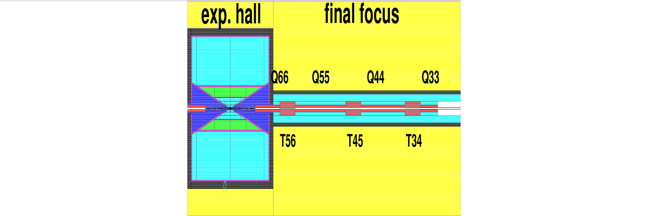
Figure 32.: Region around the Intersection Region modeled in GEANT. The black regions represent tungsten shielding. The final quadrupoles (Q) and toroids (T) on one side of the detector enclosure are shown. The shaded areas around the intersection point represent the various detector volumes used in calculating particle fluences.

The final focus may be thought to be composed of 3 separate regions. The longest of these, from 130 m to approximately 6.5 m contains the quadrupole magnets which bring the beam to the final focus in the intersection region. The space available between the four quadrupoles was used to install toroids. They fulfill a double role: first they are used as scrapers for the electromagnetic debris; secondly, they serve as magnetic deflectors for the Bethe–Heitler(BH) muons generated upstream. The effect of the toroids on the BH muons will be discussed later. In order to optimize the inner aperture of the toroids, the $\sigma_{x}$ and $\sigma_{y}$ envelope of the muon bunch at every exit of the quadrupoles has been estimated. The inner aperture of each toroid was chosen to match the 4 $\sigma$ ellipse of the muon bunch at that point.

Figure 33: Trajectories in the Final Focus Region with Muon decays turned off Figure 34: Trajectories in the Final Focus Region with Muon Decays allowed. The decay electrons are tracked until they reach either a magnet or shielding.

The second region, from 6.5 m to 1.1 m contains tungsten plus additional shielding boxes to help contain neutrons produced by photons in the electromagnetic showers. A shielding box consists of a block of Cu surrounded by polyboron. The shielding here is designed with inverted cones to reduce the probability of electrons hitting the edges of collimators or glancing off shielding surfaces (Fig. 0.4.1). The beam aperture at the entrance to this section is reduced to 2.5 cm and by the exit of the section to 4.5 mm. This profile follows the beam envelope as the particles approach the intersection region. The intersection region itself (Fig. 0.4.1) is designed as an inverse cone to prevent electrons which reach this region from hitting any shielding as this region is directly viewed by the detector. A $20^{\circ}$ tungsten cone around the intersection region is required for the reduction of the electromagnetic component of the background. The cone is lined, except very near the intersection region with polyboron to reduce the slow neutron flux. In the shielding calculations it is also assumed that there is a polyboron layer before the calorimeter and surrounding the muon system. In earlier designs this cone was only $9^{\circ}$. Whether or not the full $20^{\circ}$ is required is still under study and work is ongoing to evaluate the physics impact of this choice of the shielding cone angle. It is likely that, after optimization is completed, the cone angle will be reduced.

Figure 35: Expanded View of Region (2) near the Intersection point. The lines represent electrons from a random sample of muon decays. Figure 36: Detailed View of Region (1), the Intersection Region. The lines represent electrons from a random sample of muon decays.

Muon Decay Backgrounds.

Results using GEANT Simulation.

The backgrounds in the detector are defined as the fluence of particles (number of particles per cm² per beam crossing) across surfaces which are representative of the various kinds of detectors which might be considered. For this study the calorimeter was assumed to be a composition of copper and liquid argon in equal parts by volume which represents a good resolution calorimeter with approximately 20% sampling fraction. The other volumes of the detector were vacuum. The calorimeter starts from a radius of 150 cm and is 150 cm deep. The tracker volume is defined from 50 to 150 cm . An array of horizontal and vertical planes were placed in the detector volumes. These planes were used for flux calculations; their positions are evident in the tables of rates below.

Table 9.: Longitudinal Particle Fluences from Muon Decays and Interactions from the GEANT Calculation. Fluence = particles/cm²/crossing for two bunches of 2 10${}^{12}\mu$’s each.

Detector	Radius(cm)	$\gamma$’s	neutrons	e±	$\pi^{\pm}$	protons	$\mu^{\pm}$
Vertex	5-10	15800	2200	138	28.8	1.6	3.0
	10-15	6200	2400		7.4	0.1	1.0
	15-20	3200	2000		9.2	8.0	4.6
Tracker	20-50	900	1740		1.6	7.8	0.6
	50-100	240	1040		0.2	4.4	0.12
	100-150	260	660		0.006	0.8	0.02
Calorimeter	160-310						0.004
Muon	310-10000						0.0004

Table 10.: Radial Particle Fluences from Muon Decays and Interactions from the GEANT Calculation. Fluence = particles/cm²/crossing for two bunches of 2 10${}^{12}\mu$’s each.

Detector	Radius(cm)	$\gamma$’s	neutrons	e±	$\pi^{\pm}$	protons	$\mu^{\pm}$
Vertex	5	34000	3200	168.0	19	3.4	.7
	10	9600	3400	19	9	2.8	0.86
	15	4400	3400	4.2	4.2	2.2	0.66
	20	2500	3400		2.6	3.8	0.40
Tracker	50	880	3000		0.44	8.4	0.064
	100	320	720		0.08	1.6	0.016

Table 11.: Mean kinetic energies and momenta of particles as calculated by GEANT.

Detector	Radius	$\mu$	$\gamma$	$p$	$\pi^{\pm}$	$n$
		GeV	MeV	MeV	MeV	MeV
Vertex	10-20	24	1	30	240	10
Tracker	50-100	66	”	”	”	”
	100-150	31	”	”	”	”
Calorimeter	160-310	19	”	”	”	”

0.4.2 Detector Specifications and Design

The physics requirements of a muon collider detector are similar to those of an electron collider. The main difference has to do with the machine related backgrounds and the added shielding that is needed near the beam pipe.

At this time little detailed work has been done on the design of a complete detector. Most of the discussion has centered around the types of detector elements which might function well in this environment. The background levels detailed in the previous section are much higher than the comparable levels calculated for the SSC detectors and appear to be somewhat in excess of the levels expected at the LHC. Clearly segmentation is the key to successfully dealing with this environment. One major advantage of this muon collider over high energy hadron colliders is the long time between beam crossings; the LHC will have crossings every 25 ns compared to the 10 $\mu$s expected for the 4 TeV $\mu$-collider. Much of the detector discussion has focused on ways to exploit this time between crossings to increase the segmentation while holding the number of readout elements to manageable levels.

The real impact of the backgrounds will be felt in the inner tracking and vertex systems. One attractive possibility for a tracking system is a Time Projection Chamber (TPC)[Nygren]. This is an example of a low density, high precision device which takes advantage of the long time between crossings to provide low background and high segmentation with credible readout capability.

Silicon, if it can withstand damage from the neutron fluxes, appears to be an adequate option for vertex detection. Again, because of the time between beam crossings, an attractive option is the Silicon Drift Detector[Gatti1984]. Short drift TPC’s with microstrip[unknown] readout could also be considered for vertex detection.

An interesting question which has yet to be addressed is whether or not it is possible to tag high energy muons which penetrate the tungsten shielding which, in the present design, extends to $20^{\circ}$ from the beam axis. For example, in the case of $\mu\mu\rightarrow\nu\nu W^{+}W^{-}$ the primary physics background is due to $\mu\mu\rightarrow\mu\mu W^{+}W^{-}$. To reduce the background, in addition to a high $p_{T}$ cut on the WW pair, in might be advantageous to tag forward going muons. These $\mu$’s would penetrate the shielding.

0.4.3 Strawman Detector

Table 12.: Detector Performance Requirements.

Detector Component	Minimum Resolution/Characteristics
Magnetic Field	Solenoid; B$\geq$2 T
Vertex Detector	b-tagging, small pixels
Tracking	$\Delta$p/p${}^{2}\sim 1\!\times\!10^{-3}$(GeV)-1 at large p
	High granularity
EM Calorimeter	$\Delta$E/E$\sim 10\%/\sqrt{\rm E}\oplus 0.7\%$
	Granularity: longitudinal and transverse
	Active depth: 24 X0
Hadron Calorimeter	$\Delta$ E/E$\sim 50\%/\sqrt{\rm E}\oplus 2$%
	Granularity: longitudinal and transverse
	Total depth (EM + HAD)$\sim 7\lambda$
Muon Spectrometer	$\Delta$p/p $\sim 20\%$ 1 TeV

The detector performance criteria that are used for the design of the detector are summarized in Tb. 12. The object of this present exercise is to see if a detector can be built using state-of-the-art (or not far beyond) technology to satisfy the physics needs of the muon collider.

A layout of the strawman detector is shown in Fig. 37. A large cone ($20^{\circ}$) that is probably not instrumented and is used to shield the detector from the machine induced background.

The main features of the detector are:The element nearest to the intersection region is the vertex detector located at as small a radius as possible. A number of technologies including Silicon Drift Detectors(SDD), Silicon Pixels[ATLASTDR], and CCD detectors have been considered, as well as short drift TPC’s. SDD seem especially attractive because of the reduced number of readout channels and potentially easier construction. A micro TPC would have lower occupancy and greater radiation resistance. Tracking technologies considered were cathode pad chambers, silicon strips and TPCs. The use of a TPC is interesting as the amount of material is minimized and thus the detector does not suffer as much from low energy photon and neutron backgrounds.

Figure 37.: Strawman Detector

For the calorimeter system there are many options. A liquid argon accordion calorimeter for the EM part[ATLASTDR],[GEMTDR] and a scintillator hadronic calorimeter appear appropriate. This combination gives a hadronic resolution that is of order 50%/$\sqrt{E}$ which may be good enough. The high granularity of the EM section allows good electron identification which will be of help in tagging b-jets. In addition the longitudinal and transverse granularity allow for corrections on an event by event basis to compensate for the fact that the calorimeter is non-compensating as well as to allow the identification of catastrophic muon bremsstrahlung.

There is a single solenoid magnet, with a field of 2 T in the tracking region. The magnet is located behind the hadron calorimeter.

The muon system is a stand-alone system. The chambers in the muon system are Cathode Strip Chambers(CSC) that can be used for both a two dimensional readout as well as a trigger. These chambers have good timing resolution and relatively short drift time which minimizes neutron background problems. We now consider these components in detail:

0.4.4 Silicon Drift Vertex Detector

The best silicon detectors are capable of achieving a position resolution of 4 $\mu$m with a detector 300 $\mu$m thick. However, these results were obtained only with normally incident charged particles. For other angles of incidence, the resolution can be degraded by the fluctuations in the density of the ionization (Landau) in the silicon. The presence of a magnetic field modifies the trajectories of electrons in a silicon drift detector and normal incidence is no longer the ideal one. There is, however, a proper incidence angle which does not give any degradation of the position resolution.

The granularity of the proposed detector seems be reasonable for the rates of background particles. Based on rates in Tbs. 9,10,11, a layer located 10 cm from the beam would have 22 hits per $cm^{2}$ from the interaction of neutral particles and 32 from crossings of charged particles. For a pixel size of $316\times 316~{}\mu m^{2}$ the number of pixel per $cm^{2}$ is 1000. In this case the occupancy of background hits is less than 6%.

The damage due to the radiation dose may be a serious problem. Only about 1/3 of the neutrons have energies above 100 KeV and contribute to this damage, but the integrated flux per year for this example would still be ${\rm 3\ 10^{14}\ n^{\prime}s\ cm^{-2}year^{-1}}$. If detectors are produced from an n–type silicon with a bulk doping level of $1.5\times 10^{12}/cm^{3}$ the detectors would have to be replaced after a year of operation. The use of p–type material seems to be more appropriate for this application. P–type silicon drift detectors are being developed in LBNL. These detectors are supposed to be much more radiation resistant. Some R&D may be required.

0.4.5 Time Projection Chamber (TPC)

An interesting candidate for tracking at a muon collider is a Time Projection Chamber (TPC). This device has good track reconstruction capabilities in a low density environment, good 3-dimensional imaging and provides excellent momentum resolution and track pointing to the vertex region. It is perhaps particularly well suited to this environment as the long time between bunch crossings ($\sim 10~{}\mu$s) permits drifts of $\sim$1 m and the average density of the device is low compared to more conventional trackers which helps to reduce the measured background rates in the device. In the present detector considerations the TPC would occupy the region between the conic tungsten absorber and electromagnetic calorimeter in the region from 35 cm to 120 cm, divided into two parts, each 1 m long.

To reduce background gamma and neutron interactions in the detector volume, a low density gas mixture should be chosen as the detection medium of the TPC. Another important parameter is the electron drift velocity. Since the time between beam crossings is fixed (10 $\mu$s in the present design) the drift velocity should be high enough to collect all the ionization deposited in the drift region. Finally the detection medium should not contain low atomic number gases to help reduce the transfer energy to the recoil nucleus and in this way to reduce its range in the gas. The gas mixture 90% He + 10% CF₄ satisfies all these requirements and could be an excellent candidate. It does not contain hydrogen which would cause a deleterious effect from the neutrons, has a density $1.2$ mg/cm³ and a drift velocity of 9.4 cm/$\mu$s. The single electron longitudinal diffusion for this gas is

$$\sigma_{l}=0.15\,{\rm mm}/\sqrt{\rm cm}.$$ (15)

The transverse diffusion, which is strongly suppressed by the 2 T magnetic field is given by,

$$\sigma_{t}=\frac{\sigma_{t}(B=0)}{\sqrt{1+(\omega\tau)^{2}}}=0.03\,{\rm mm}/{\sqrt{\rm cm}}$$ (16)

Each time slice will contain about 25 ionization electrons, and the expected precision in r- $\phi$ and z coordinates is,

$$\sigma_{\phi}=\sqrt{\frac{Z\sigma_{t}^{2}}{25}+(50)^{2}}\approx 100\,({\rm\mu m})\qquad\sigma_{Z}=\sqrt{\frac{Z\sigma_{l}^{2}}{25}+(150)^{2}}\approx 300\,({\rm\mu m})$$ (17)

where Z, the drift length is 1 m. The precision of r-coordinate is defined by the anode wire pitch - 3 mm.

Occupancy from Photons.

Low energy photons, neutrons and charged particles produce the main backgrounds in the tracker. Photons in the MeV region interact with matter mainly by Compton scattering. For a 1 MeV photon the probability of producing a Compton electron in 1 cm of gas is $\xi_{\gamma}=4.5\times 10^{-5}$. For an average photon fluence $h_{\gamma}=200$ cm^-2 about $N_{\gamma}=8\times 10^{4}$ electron tracks are created in the chamber volume. Because the transverse momentum of Compton electrons is rather small the electrons are strongly curled by the magnetic field and move along the magnetic field lines. Most of the electrons have a radius less than one millimeter and their projection on the readout plane covers not more than one readout pitch, $0.3\times 0.4$ cm². The average length of the Compton electron tracks in the TPC is 0.5 meter and therefore, the volume occupied by electron tracks is $v_{comp.e}=4.8\times 10^{5}$ cm³. Since the total chamber volume is $10^{7}$ cm³, the average occupancy due to background photon interactions is equal to,

$$\ <occupancy>_{\gamma}=\frac{V_{comp.e}}{V_{total}}=4.4\times 10^{-2}$$ (18)

and could be further reduced by subdividing the chamber in length, thus shortening the drift distances. Indeed this may be required to reduce an excessive space charge distortion from the accumulation of ions.

These Compton tracks can easily be identified and removed. Because almost all points of a Compton track lie along the $z$-axis most of them will be projected into one cell and therefore the number of points in this cell will be very different from hit cells from non-background tracks. To remove low momentum electron tracks, all cells containing more than some threshold number of points should be excluded. Applying this procedure a few percent of volume is lost but the quality of the high momentum tracks is not substantially changed. This is illustrated in Fig. 38 where one sector of the TPC is shown after the application of different value threshold cuts.

Occupancy from Neutrons.

For neutrons in the MeV region the primary interaction with matter is elastic collisions. In this case the energy transfer to the nucleus has a flat distribution and the maximum transfer energy is given by $4E_{n}A/(A+1)^{2}$ or $4E_{n}/A$ when $A\gg 1$.

The calculated mean energy of background neutrons is $E_{n}=27$ $MeV$. In this case, for hydrogen, their mean range in the gas is several meters, but for the gas chosen, the mean length of the recoil nucleus tracks will only be a few millimeters.

The calculated neutron fluence is $<n>=2\times 10^{3}$ ${cm^{-2}}$. The track of the recoil nucleus occupies, typically, not more than one volume cell of the TPC, $v_{n}=0.3\!\times\!0.4\times 1.0$ cm³. The probability of a background neutron interacting in 1 cm of the gas is $\xi_{n}=2\times 10^{-5}$, the number of recoil tracks $N_{n}=<n>\cdot\xi_{n}\cdot V_{total}=4\times 10^{5}$ and therefore the neutron occupancy is,

$$\ <occupancy>_{n}=\frac{N_{n}\cdot v_{n}}{V_{total}}=0.48\times 10^{-2}$$ (19)

It is easy to clean out these recoil tracks owing to their large ionization density per cell. Only a simple cut to remove all volume cells which contain a charge in excess of some preset threshold is required. This cut will only eliminate about 1% of the TPC volume.

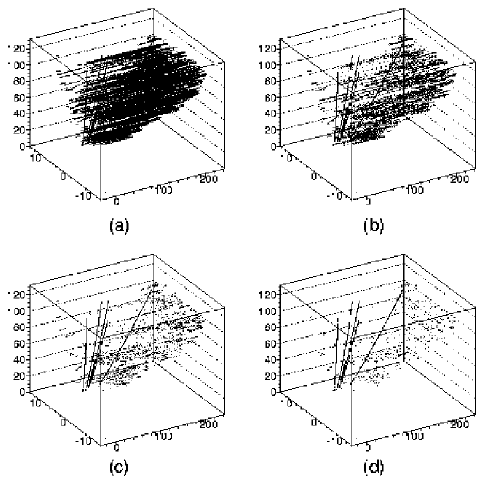
Figure 38.: Charge distribution from a signal event and background Compton electrons with threshold cuts; (a) has no cut applied while (d) has the most stringent cut.

0.4.6 Micro TPC for vertex detection

TPCs with very short drift distances (3 cm) and microstrip readout (0.2 x 2 mm pads) might be an interesting alternative to silicon drift chambers for vertex detection. The resolution of such chambers would be somewhat worse (of the order of $30\,\mu$m, compared with $4\,\mu$m), but the greater number of points would compensate for this to some extent. Such chambers would have less occupancy and much greater radiation resistance than silicon devices.

0.4.7 Electromagnetic Calorimeter

An accordion liquid argon calorimeter is being developed for the ATLAS collaboration[ATLASTDR]. A similar calorimeter designed for the GEM Collaboration at the SSC.

From the GEANT background calculations, the total energy deposited from the electromagnetic debris is $\sim$ 13 TeV but relatively uniformly distributed. If one divides the calorimeter into $\sim 2\!\times\!10^{5}$ cells, the mean energy would be about 65 MeV/cell. Certainly, energetic electromagnetic showers from $\gamma$’s or electrons or the core of jets will stand out above this uniform noise. Since the readout is every 10 $\mu$s, multiplexing is possible to reduce costs compared to the LHC where collisions occur every 25 ns.

0.4.8 Hadron Calorimeter

A good choice for the hadron calorimeter is a scintillator tile device being designed for ATLAS[ATLASTDR]. It uses a novel approach where the tiles are arranged perpendicular to the beam direction to allow easy coupling to wave-length shifting fibers[Guildermeister]. With a tile calorimeter of the type discussed here it should be possible to achieve a resolution of $\Delta$ E/E$\sim 50\%/\sqrt{\rm E},$ satisfying the requirements in Tb. 12.

From the GEANT background calculations, the total energy deposited in the calorimeter from electromagnetic and hadronic showers and muons is about 200 TeV. Again, this is rather uniform with and if subdivided into $10^{5}$ towers would introduce 2 GeV pedestals with 300 MeV fluctuations: also acceptable. But the muons, arising from Bethe-Heitler pair production in EM showers or from a halo in the machine, though modest in number, have high average energies. They would not be a problem in the tracking detectors, but in the calorimeters, they would occasionally induce deeply inelastic interactions, depositing clumps of energy deep in the absorbers. If a calorimeter is not able to recognize the direction of such interactions (they will be pointing along the beam axis) then they would produce unacceptable fluctuations in hadron energy determination. Segmenting the calorimetry in depth should allow these interactions to be subtracted. We are studying various solutions, including the use of fast time digitizing[jsand] to provide such segmentation, but ultimately there will have to be some hardware tests to verify the MC study.

0.4.9 Muon Spectrometer

Triggering is probably the most difficult aspect of muon spectrometers in large, 4$\pi$ detectors in both lepton and hadron colliders. In addition, a muon system should be able to cope with the larger than usual muon backgrounds that would be encountered in a muon collider. Segmentation is, again, the key to handling these high background rates. Cathode Strip Chambers (CSC) are an example of a detector that could be used in the muon system of a muon collider experiment. This detector performs all functions necessary for a muon system:

• Precision coordinate(50 to 70 $\mu$m)

• Transverse coordinate(of order mm or coarser as needed)

• Timing (to a few ns)

• Trigger primitives

In addition, the cathodes can be lithographically segmented almost arbitrarily resulting in pixel detectors the size of which is limited only by the density and signal routing of the readout electronics.

0.4.10 Halo Background

There could be a very serious background from the presence of even a very small halo of near full energy muons in the circulating beam. The beam will need careful preparation before injection into the collider, and a collimation system will have to be designed to be located on the opposite side of the ring from the detector.

0.4.11 Pair Production

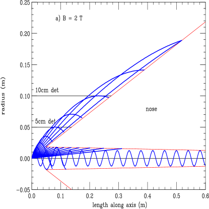
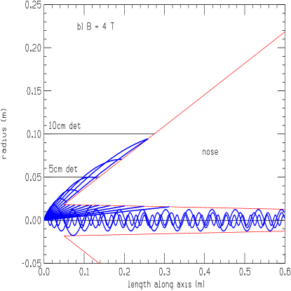
Figure 39.: Radius vs. length of electron pair tracks for initial momenta from 3.8 to 3000 MeV in geometric steps of $\sqrt{2};$ (a) for a solenoid field of 2 T, (b) for 4 T.

There is also a background from incoherent (i.e. $\mu^{+}\mu^{-}$ $\rightarrow$ $e^{+}e^{-}$) pair production in the 4 TeV Collider case[ref37]. The cross section is estimated to be $10\,$mb[ginzburg], which would give rise to a background of $\approx 3\times 10^{4}$ electron pairs per bunch crossing. The electrons at production, do not have significant transverse momentum, but the fields of the oncoming 3 $\mu$m bunch can deflect them towards the detector. A simple program was written to track electrons from close to the axis (the worst case) as they are deflected away from the bunch center. Once clear of the opposing bunch, the tracks spiral under the influence of the experimental solenoid field. Fig. 39 (a) shows the radii vs, length of these electron tracks for initial momenta from 3.8 to 3000 MeV in geometric steps of $\sqrt{2}$ and a solenoid field of 2 T, see Fig.39a ( Fig. 39b it is 4 T). In the 2 T case, tracks with initial energy below 30 MeV do not make it out to a detector at 10 cm, while those above 100 MeV have too small an initial angle and remain within the shield. Approximately $10\ \%(3000)$ of these are in this energy range and pass through a detector at 10 cm. The track fluence at the ends of the detector are less than 10 tracks per cm² which should not present a serious problem. At 5 cm, there are 4500 tracks giving a fluence of 30 per cm², which is also probably acceptable. If the detector solenoid field is raised to 4 T then no electrons reach 10 cm and the flux at 5 cm is reduced by a factor of 2.

There remains some question about the coherent pair production generated by virtual photons interacting with the coherent electromagnetic fields of the entire oncoming bunch. A simple Weizsäcker-Williams calculation[ref37] yields a background that would consume the entire beam at a rate comparable with its decay. However, I. Ginzburg[ginzburg] and others have argued that the integration must be cut off due to the finite size of the final electrons. If this is true, then the background becomes negligible. A more detailed study of this problem is now underway[chen][pisin].

If the coherent pair production problem is confirmed, then there are two possible solutions:

1) one could design a two ring, four beam machine (a $\mu^{+}$ and a $\mu^{-}$ bunch coming from each side of the collision region, at the same time). In this case the coherent electromagnetic fields at the intersection are canceled and the pair production becomes negligible.

2) plasma could be introduced at the intersection point to cancel the beam electromagnetic fields[plasma].

0.4.12 Detector and Background Conclusions.

Two independent background calculations have been used for a preliminary study of the expected background level at a 4 TeV muon collider. The optimization of the intersection region is still at its infancy, but the results of both studies show that the level of background while still large, can be managed with proper design of the intersection region and choice of detector technologies. This is in large part due to the fact that the background is composed of many very soft particles which behave like a pedestal shift in the calorimeter. The tracking and vertexing systems will have to be highly segmented to handle this flux of background particles.

A large amount of work is still needed in order to optimize the intersection region and the final focus. In particular a better understanding of the trade off between the different backgrounds is required. The strawman detector is meant only to show that the muon collider detector has unique problems and advantages. An optimized detector needs to be developed taking these problems into consideration.

Some preliminary calculations for machine related backgrounds for a lower energy collider (250 GeV x 250 GeV) have also been carried out. It appears that the backgrounds in this case are comparable to those at the 4 TeV machine. Since little attention has yet been paid to the details of the final focus for this lower energy machine it is possible that reductions in the machine related backgrounds will be achievable in the future.

0.5 OPTIONS

0.5.1 Introduction

Up to this point, this report has concentrated on the design of a muon collider with

1) beam energies of 2 + 2 TeV

2) operating at its maximum energy

3) with a fixed rms energy spread of 0.12

4) with no attention to maximizing polarization

In this section we discuss modifications to enhance the muon polarization’s, operating parameters with very small momentum spreads, operations at energies other than the maximum for which a machine is designed, and designs of machines for different maximum energies.

0.5.2 Polarization

Polarized Muon Production.

The specifications and components in the baseline design have not been optimized for polarization. Nevertheless, simple manipulations of parameters and the addition of momentum selection after phase rotation does generate significant polarization with relatively modest loss of luminosity. The only other significant changes required to give polarization at the interaction point are rotators in the transfer lines, and a chicane snake in the collider opposite the IP.

Figure 40.: Polarization in the lab. frame vs. the cosine of the center of mass decay angle, for a number of pion energies.

In the center of mass of a decaying pion, the outgoing muon is fully polarized (-1 for $\mu^{+}$ and +1 for $\mu^{-}$). In the lab system the polarization depends[decaypolar] on the decay angle $\theta_{d}$ and initial pion energy. Figure 40 shows this polarization as a function of the cosine of the center of mass decay angle, for a number of pion energies. It is seen that for pion kinetic energy larger than the pion mass, the dependence on pion energy becomes negligible and the polarization is given approximately by:

$$P_{\mu^{-}}\approx\cos{\theta_{d}}+0.28(1-\cos^{2}{\theta_{d}})$$ (20)

The average value of this is about 0.19. A Monte Carlo calculation[mc] of the capture, decay and phase rotation discussed above gave muon polarization of approximately 0.22. The slight difference of this value from the average comes from an accidental bias towards forward decay muons.

If higher polarization is required, some deliberate selection of muons from forward pion decays $(\cos{\theta_{d}}\rightarrow 1)$ is required. This could be done by selecting pions within a narrow energy range and then selecting only those muons with energy close to that of the selected pions. But such a procedure would collect a very small fraction of all possible muons and would yield a very small luminosity. Instead we wish, as in the unpolarized case, to capture pions over a wide energy range, allow them to decay, and to use rf to phase rotate the resulting distribution.

Consider the distributions in velocity vs. ct at the end of a decay channel. If the source bunch of protons is very short and if the pions were generated in the forward direction, then the pions, if they did not decay, would all be found on a single curved line. Muons from forward decays would have gained velocity and would lie above that line. Muons from backward decays would have lost velocity and would fall below the line. A real distribution will be diluted by the length of the proton bunch, and by differences in forward velocity due to the finite angles of particles propagating in the solenoid fields. In order to reduce the latter, it is found desirable to lower the solenoid field in the decay channel from 5 to 3 Tesla. When this is done, and in the absence of phase rotation, one obtains the distribution shown in Fig. 41, where the polarization P$>{1\over 3}$, $-{1\over 3}<P<{1\over 3}$, and P$<-{1\over 3}$ is marked by the symbols ‘+’, ‘.’ and ‘-’ respectively. One sees that the +’s are high, and the -’s are low, all along the distribution.

Figure 41.: Energy vs. ct of $\mu$’s at end of decay channel without phase rotation; muons with polarization P$>{1\over 3}$, $-{1\over 3}<P<{1\over 3}$, and P$<-{1\over 3}$ are marked by the symbols ‘+’, ‘.’ and ‘-’ respectively.

It is found that phase rotation does not remove this correlation: see Fig. 42. Now, after time cuts to eliminate decays from high and low energy pions, there is a simple correlation of polarization with the energy of the muons.

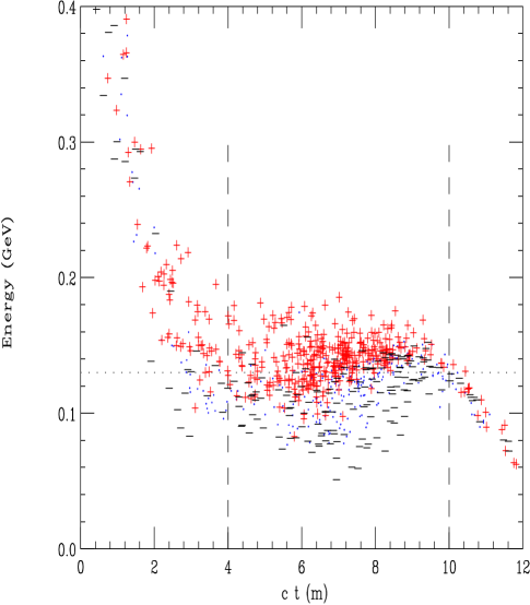
Figure 42.: Energy vs. ct of $\mu$’s at end of decay channel with phase rotation; muons with polarization P$>{1\over 3}$, ${-1\over 3}<P<{1\over 3}$, and P$<{-1\over 3}$ are marked by the symbols ‘+’, ‘.’ and ‘-’ respectively.

If a selection is made on the minimum energy of the muons, then net polarization is obtained. The higher the cut on energy, the greater the polarization, but the less the fraction $F_{loss}$ of muons that are selected. The cut in time can probably be obtained from the phasing of the rf used to capture the bunch. Alternatively, it could be provided by a second energy cut applied after a 90 degree longitudinal phase rotation.

In order to provide the required cut on energy, one needs to generate dispersion that is significantly larger than the beam size. Collimation from one side can then select the higher energy muons. After collimation, the remaining dispersion should be removed. The generation of sufficient dispersion, in the presence of the very large emittance, is non-trivial. The only practical method appears to be the use of a bent solenoid (as discussed above, in the section of Muon Collider Components). First the solenoid is bent one way to generate the dispersion; the collimator is introduced; then the solenoid is bend the other way to remove the dispersion. The complete system thus looks like an “S” or “snake”. Particles with momentum $p_{\mu}$ in a magnetic field $B$ have a bending radius of $R_{B}$, given by:

$$R_{B}={\left({ep_{\mu}/mc}\right)\over c\ B}.$$ (21)

If the particles are trapped in a solenoid with this field, and the solenoid is bent with a radius $R_{bend}$, where $R_{bend}>>R_{B},$ then those particles, besides their normal helical motion in the solenoid, will drift in a direction ($z$) perpendicular to the bend, with a drift angle ($\theta_{drift}=dz/ds$) given by:

$$\theta_{drift}\ \approx\ {R_{B}\over R_{bend}}$$ (22)

The integrated displacement in $z$, ie. the dispersion $D$, is then:

$$D\ =\ \theta_{drift}\ s\ \approx\ \phi\ R_{B},$$ (23)

where $\phi$ is the total angle of solenoid bend.

As an example, we have traced typical particles with momenta of 150 and 300 MeV/c through a snake with $B=1\,T$, $R_{bend}=6\ m,$ with a first band with $\phi=\pi$ followed by a reverse bend $\phi=-\pi.$ Fig. 43 shows the trajectories of muons as viewed from the z direction. No significant dispersion is seen. The two momenta are seen to be dispersed during the right hand turn and recombined by the left hand turn.

Figure 43.: Dispersion Snake: trajectories as seen from the $z$ direction (top); vertical (z) particle positions vs. length (s) along the snake (bottom).

Fig. 44 and Tb. 13 give the results of a Monte Carlo study[mc] in which dispersion is introduced, and progressive cuts are applied, to the muons at the end of the phase rotation. In this calculation, in order to calculate more rapidly, the trajectories were not actually traced through a snake. Instead, the particles were propagated through 20 m of straight solenoid, followed by the application of dispersion equal to 6 times the momentum in GeV/c. A snake that would give such dispersion could have the parameters: solenoid field of 3 T (giving $R_{B}=0.25\ m$ at the average momentum of 230 MeV/c), diameter of snake bends greater than 5 m and bend angles of $320^{\circ},$ (which would require some variations in bend curvature to avoid the solenoid crossing itself),

Tb. 13 gives results for two fields in the decay channel solenoids: 5 T, the field in the point design; and 3 Tesla, chosen to increase the polarization. It is seen that for weak cuts and small polarization, it is better to avoid the loss of muons from the lower, 3 T, field, but with stronger cuts, the lower field gives greater polarization. In Fig. 44, and subsequent plots, only data from the preferred fields are shown beyond the cross over.

Table 13.: Production Polarization vs. Position. B, decay channel field; cut, the position of the colimator; $P_{init}$ initial polarization; $P_{final}$ polarization after dilution in the cooling section; $P_{vec}$ effective vector polarization (see Eq.26); $R_{v/s}$ vector to scalar ratio (see Eq.27); $L_{vec}$ luminosity enhancement for vector state; $E_{ave}$ average final muon energy; $\Delta$E rms final energy spread

B	cut	$F_{loss}$	$P_{init}$	$P_{final}$	$P_{vec}$	$R_{v/s}$	$L_{vec}$	$E_{ave}$	$\Delta$E
T	m							MeV	MeV
5	0.00	1.000	0.23	0.18	0.36	1.45	1.18	130	23
5	1.00	0.960	0.27	0.21	0.41	1.54	1.21	144	23
5	1.12	0.890	0.30	0.24	0.46	1.64	1.24	147	20
5	1.24	0.759	0.36	0.29	0.53	1.80	1.29	151	18
5	1.30	0.614	0.41	0.33	0.60	1.99	1.33	157	17
5	1.40	0.360	0.48	0.39	0.67	2.26	1.39	166	15
5	1.50	0.163	0.56	0.45	0.75	2.64	1.75	177	15
3	0.00	0.801	0.22	0.18	0.34	1.43	1.18	130	22
3	1.06	0.735	0.29	0.23	0.44	1.61	1.23	133	22
3	1.16	0.673	0.35	0.28	0.52	1.77	1.28	137	19
3	1.26	0.568	0.41	0.33	0.59	1.98	1.33	141	17
3	1.32	0.417	0.50	0.40	0.69	2.32	1.40	147	15
3	1.40	0.264	0.59	0.47	0.77	2.78	1.47	151	13
3	1.48	0.126	0.70	0.56	0.86	3.58	1.56	159	13
3	1.56	0.055	0.77	0.62	0.90	4.25	1.62	168	12

Figure 44.: Polarization vs. $F_{loss}$ of muons accepted; the dashes show polarization as selected, the line gives polarization after cooling.

It is seen from Tb. 13 that the energy cut not only increases the polarization, but also decreases the energy spread $\Delta E$ of the remaining muons. In Fig. 45 the fractional energy spread $\Delta E/E$ is plotted against the loss factor $F_{loss}$. The energy spread is reduced almost a factor of two for reasonable collimator positions. This reduction in energy spread would eliminate the need for the first stage of emittance cooling.

Figure 45.: the fractional energy spread $\Delta E/E$ is plotted against the loss factor $F_{\rm loss}$.

A Monte Carlo study has also been done on the effect of variations of the proton bunch length $\sigma_{t}$. Fig. 46a shows the polarization before cooling as a function of $\sigma_{t}$ for three values of the loss factor $F_{loss}$. It is seen that serious loss of polarization can occurs when the rms width is more than 1 nsec. Fig. 46b shows the muon rms energy spread after the polarization cut. Again it is shown as a function of $\sigma_{t}$ for three values of the loss factor $F_{loss}$. With no cut, the rise in energy spread would be serious ($\Delta E>20\,{\rm MeV}$ is difficult to cool) for an rms width more than 1 ns. But with polarization cuts, the energy spread is so reduced that a larger proton bunch length would not be a problem.

Figure 46.: Polarization vs $\sigma_{t},$ the proton bunch length (upper plot). Muon rms energy spread vs. $\sigma_{t}$ (lower plot). Both plots for three values of the loss factor $F_{\rm loss}.$

0.5.3 Polarization Preservation

A recent paper[rossmanith] has discussed the preservation of muon polarization in some detail. During the ionization cooling process the muons lose energy in material and have a spin flip probability ${\cal P},$ where

$${\cal P}\approx\int{{m_{e}}\over{m_{\mu}}}\beta_{v}^{2}\ {\Delta E\over E}$$ (24)

where $\beta_{v}$ is the muon velocity divided by c, and $\Delta$E/E is the fractional loss of energy due to ionization. In our case the integrated energy loss is approximately 3 GeV and the typical energy is 150 MeV, so the integrated spin flip probability is close to 10%. The change in polarization $dP/P$ is twice the spin flip probability, so the reduction in polarization is approximately 20 %. This dilution is included in the “$P_{final}$” column in Tb. 13 and is plotted as the line in Fig. 44.

During circulation in any ring, the muon spins, if initially longitudinal, will precess by $(g-2)/2\gamma$ turns per revolution in the ring; where $(g-2)/2$ is $1.166\times 10^{-3}$. An energy spread $d\gamma/\gamma$ will introduce variations in these precessions and cause dilution of the polarization. But if the particles remain in the ring for an exact integer number of synchrotron oscillations, then their individual average $\gamma$’s will be the same and no dilution will occur. It appears reasonable to use this “synchrotron spin matching”[rossmanith] to avoid dilution during acceleration.

In the collider, however, the synchrotron frequency will be too slow to use “synchrotron spin matching”, so one of two methods must be used.

• Bending can be performed with the spin orientation in the vertical direction, and the spin rotated into the longitudinal direction only for the interaction region. The design of such spin rotators appears relatively straightforward. The example given in the above reference would only add 120 m of additional arc length, but no design has yet been incorporated into the lattice.

• The alternative is to install a Siberian Snake[siberian] at a location exactly opposite to the intersection point. Such a snake reverses the sign of the horizontal polarization and generates a cancelation of the precession in the two halves of the ring.

Provision must also be made to allow changes in the relative spins of the two opposing bunches. This could be done, prior to acceleration, by switching one of the two beams into one or the other of two alternative injection lines.

0.5.4 Benefits of Polarization of Both Beams

We consider two examples of the general advantage of having polarization in both beams. Individual physics experiments would have to be considered to determine how important such advantages are.

Consider the polarization of a vector spin state generated by the annihilation of the two muons.

$$P_{vec}\ =\ {F^{++}-F^{--}\over F^{++}+F^{--}}$$ (25)

When only one beam has polarization $P_{1}$, then $P_{vec}=P_{1}$. But if both beams have polarization $P$ in the same direction (ie. with opposite helicities), then

$$P_{vec}\ =\ {(P+1)^{2}-(P-1)^{2}\over(P+1)^{2}+(P-1)^{2}}$$ (26)

In Fig. 47 both the polarization of each beam $P$, and the resulting polarization of a vector state $P_{vector}$ are plotted against the loss factor $F_{loss}$.

Figure 47.: Polarization of each beam $P$, and the resulting polarization of a vector state $P_{vec}$ vs. the loss factor $F_{loss}$.

A second advantage is that the ratio $R_{v/s}$ of vector to scalar luminosity can be manipulated to enhance either the vector or the scalar state. If the polarization directions have been chosen to enhance the ratio of vector to scalar states, then:

$$R_{v/s}\ =\ {1+P\over 1-P}.$$ (27)

Tb. 13 and Fig. 48 show this ratio as a function of the loss factor $F_{loss}$.

Figure 48.: Ratio of vector to scalar states, $R_{v/s}$ vs. the loss factor $F_{loss}.$

Tb. 13 also shows that the fraction of total luminosity in a given state can be enhanced. If polarizations are chosen to enhance the vector state, then the fraction of vector luminosity is increased from 1/2 to $(1+P)/2$, giving a gain factor of

$${\cal L}_{vec}=1+P$$ (28)

0.5.5 Luminosity loss

If nothing else is done, then the luminosity, which is proportional to $n_{\mu},$ will drop as $F_{loss}^{2}$; where $F_{loss}$ is the fraction muons lost by the muon momentum cut. At the same time, however, the space charge, wakefield, and loading during the cooling and acceleration will all be reduced; as will the beam beam tune shift in the collider. Clearly, the machine parameters should be reoptimized and some part of the lost luminosity recovered.

One way to recover the luminosity would be to increase the proton bunch intensity by the factor $F_{loss}$. If this were done, then the original number of muons per bunch would be generated; all the wake field, loading and space charge effects would be the same; and the luminosity per bunch crossing would be the same. If we assume that the total proton current is determined by the driver, then such an increase in proton intensity per bunch will necessitate a reduction in the number of bunches or repetition rate, by the same factor $F_{loss}$. The luminosity will then fall by $F_{loss}$ and not by $F_{loss}^{2}$ as before.

For instance, in the unpolarized case of the $4\,$TeV collider, there were two bunches of each sign. If the momentum cut is chosen to give a value of $F_{loss}$ = 1/2, and the proton beam is distributed into 2 instead of 4 initial bunches, then the final number of muons per bunch, the loading, beam beam tune shift, etc. would all be the same as in the unpolarized case. The luminosity would be down by a factor of only two, for a polarization of 34 % in both beams.

For higher polarization at good luminosity it would be desirable to have a proton source with the option of a lower repetition rate, but even larger numbers of protons per spill. For example 4 x $10^{14}$ protons per pulse at 4 Hz. It should then be possible to extend this method to an operation with $F_{loss}$ = 1/8, and polarization of both beams of 57 %.

One also notes that the luminosity could be maintained at the full unpolarized value if the proton source intensity could be increased. Such an increase in proton source intensity in the unpolarized case would be impractical because of the resultant excessive high energy muon beam power, but this restriction does not apply if the increase is used to offset losses in generating polarization. If, for instance, the driver repetition rate were increased from 15 to 30 Hz, the fractions $F_{loss}$ set at 0.5, and the number of bunches reduced to one, then the full luminosity of $10^{35}\ (cm^{-2}s^{-1})$ would be maintained with polarization of both beams of 34%.

0.5.6 Luminosity

The bunch populations decay exponentially, yielding an integrated luminosity equal to its initial value multiplied by an effective number of turns $n_{{\rm eff}}\approx 150\ B,$ where B is the mean bending field in T.

The luminosity is given by:

$$\cal L\rm\ =\ {n_{\mu}^{2}\ n_{b}f_{rep}\ n_{eff}\gamma\over 4\pi\ \beta_{\perp}^{*}\ \epsilon_{n}}H(A,D)$$ (29)

where $n_{\mu}$ is the number of muons per bunch, $n_{b}$ is the number of bunches, $\gamma$ is the normalize energy, $\beta_{\perp}^{*}$ is the beta function at the IP and $\epsilon_{n}$ is the transverse normalize emittances (assumed vertical and horizontal to be equal), and the enhancement factor $H(A,D)$ is

$$H(A,D)\approx 1+D^{1/4}\left[{D^{3}\over 1+D^{3}}\right]\left\{\ln{(\sqrt{D}+1)}+2\ln{({0.8\over A})}\right\},$$ (30)

$$A=\sigma_{z}/\beta^{*},$$ (31)

and

$$D={\sigma_{z}n_{\mu}\over\gamma\sigma_{t}^{2}}r_{e}({m_{e}\over m_{\mu}})$$ (32)

In the cases we are considering[pisin2]: A = 1, D $\approx$ .5 and H(A,D) $\approx 1$.

0.5.7 Luminosity vs. Energy, for a Given Ring

For a fixed collider lattice, operating at energies lower than the design value, the luminosity will fall as $\gamma^{3}.$ One power comes from the $\gamma$ in Eq. 29; a second comes from $n_{eff}$, the effective number of turns, that is proportional to ${\gamma}$; the third factor comes from $\beta^{*},$ which must be increased proportional to $\gamma$ in order to keep the beam size constant within the focusing magnets. The bunch length $\sigma_{z}$ must also be increased proportional to $\gamma$ so that the required longitudinal phase space is not decreased; so A = $\sigma_{z}/\beta^{*}$ remains constant.

0.5.8 Scaling for Collider Rings for Different Energies

As noted above, the luminosity in a given ring will fall as the third power of the energy at which it is operated. Such a drop is more rapid than the gain in typical cross sections, and, as we shall see, it is more rapid than the drop in luminosity obtained with rings designed for the lower energies. It would thus be reasonable, having invested in a muon source and accelerator, to build a sequence of collider rings at spacings of factors of 2-3 in maximum energy. We will now derive scaling rules for such collider rings.

The luminosity

$${\cal L}\ =\ {n_{\mu}^{2}\ n_{\rm eff}\ n_{b}\ f_{\rm rep}\ \gamma\over 4\ \pi\ \epsilon_{n}\ \beta_{\perp}^{*}}\ \propto\ {n_{\mu}\ I_{\mu}\ \gamma\over\epsilon_{n}\ \beta^{*}}$$ (33)

where $I_{\mu}=n_{\mu}n_{b}f_{rep},$ is the muon flux and which, since $\Delta\nu_{bb}$, the beam beam tune shift is given by:

$$\Delta\nu_{bb}\ \propto\ {n_{\mu}\over\epsilon_{n}},$$ (34)

gives:

$${\cal L}\ \propto\ {I_{\mu}\ \Delta\nu_{bb}\ \gamma\over\beta_{\perp}^{*}}$$ (35)

If a final focus multiplet is scaled keeping the relative component lengths and the pole tip fields constant, then one obtains:

$$\ell^{*}\ \propto\ \sqrt{a_{max}\ \gamma}$$ (36)

$$\theta^{*}\ \propto\ \sqrt{{a_{max}\over\gamma}}\propto\ \sqrt{{\epsilon_{n}\over\beta_{\perp}^{*}\ \gamma}}$$ (37)

$$\beta_{\perp}^{*}\ \propto\ {\epsilon_{n}\over a_{max}}$$ (38)

where $\theta^{*}$ is the rms angle of muons diverging from the focus, $\ell^{*}$ is the free space from the target to the first quadrupole (proportional to all quadrupole lengths in the multiplet), and $a_{max}$ is the maximum aperture of any quadrupole (proportional to all apertures in the multiplet).

The normalized emittance $\epsilon_{n}$ is constrained by the ionization cooling, but since one can exchange transverse and longitudinal emittance, it is, in principle, the six dimensional emittance $\epsilon_{6}$ that is constrained. Extending the lepton emittance conventions, we define:

$$\epsilon_{6}\ =\ (\epsilon_{n})^{2}\ {dp\over p}\sigma_{z}\gamma\beta_{v}.$$ (39)

With this definition, the six dimensional phase space $\Phi_{6}\ =\ \pi^{3}\ m_{\mu}^{3}\ \epsilon_{6}$. $\sigma_{z}$ cannot be large compared with the focus parameter $\beta^{*}$, so, taking them to be proportional to one another, and taking the $\beta_{v}=1$, then:

$$\epsilon_{6}\ \propto\ (\epsilon_{n})^{2}\ {dp\over p}\beta^{*}\gamma$$ (40)

and from the above:

$$(\epsilon_{n})^{3}\ \propto\ {\epsilon_{6}\ a_{max}\over\gamma\ {dp\over p}}$$ (41)

$$(\beta_{\perp}^{*})^{3}\ \propto{\epsilon_{6}\over\gamma\ {dp\over p}\ a_{max}^{2}}$$ (42)

0.5.9 Six Dimensional Emittance dependence on $n_{\mu}$ and $\epsilon_{n}$

The six dimensional emittance $\epsilon_{6}$ obtained from the cooling will, because of more detailed constraints, depend to some extent on the number of muons $n_{\mu}$, and on the final transverse emittance $\epsilon_{n}$.

The approximate dependence on the number of muons is relatively transparent. As the number of muons per bunch rises, the longitudinal space charge forces increase and it becomes impossible, without changing the rf gradients, to maintain the same bunch lengths. As a result the bunch lengths must be increased by the square root of the number of muons.

A study, with the analytic formulae used for the model cooling system discussed before, was used again to derive cooling sequences with different final parameters. First, sequences were calculated with numbers of initial muons per bunch of 1, 2, 3.75, 7.5, and 15 x $10^{12}$ (corresponding to muons in the collider of 0.1, 0.2, 1, 2, and 4 x $10^{12}$). The final transverse emittance at the end of the cooling was required to be $4\times 10^{-5}$ m, (corresponding to an emittance in the collider of $5\times 10^{-5}$ m). The six dimensional emittances obtained are plotted in Fig. 49a. It is seen that for $n_{\mu}>10^{12}$ the six dimensional emittances are indeed approximately proportional to the root of the number of muons (the line shows this dependence).

The study also obtained cooling sequences giving six dimensional emittances for a range of final transverse emittances. The dependence here is more complicated. If emittance exchange between longitudinal and transverse emittances could be achieved without material then the six dimensional emittance should be independent of the final transverse emittance chosen. But the exchange does require material and Coulomb scattering in this material increases the six dimensional emittances; and it does so to a greater extent if the transverse emittance is small. In Fig. 49b, we show the six dimensional emittances obtained for 5 representative transverse emittances. Over the range of interest the dependence of $\epsilon_{6}$ is approximately the inverse root of $\epsilon_{n}$ (the line shows this dependence).

For the purposes of this study, we may thus assume that:

$$\epsilon_{6}\ \propto\ \sqrt{n_{\mu}\over\epsilon_{n}}$$ (43)

Figure 49.: Six dimensional emittance $\epsilon_{6}$ vs. a) muon intensity $n_{\mu}$ entering the cooling, and b) the transverse emittance $\epsilon_{n}$ at the end of the cooling

0.5.10 Energy Scaling, allowing the emittances to vary

If $n_{\mu}$ is limited by the beam beam tune shift:

$$n_{\mu}\ \propto\ \epsilon_{n}\ \Delta\nu_{bb}$$ (44)

substituting this in Eq. 43:

$$\epsilon_{6}\ \propto\ \sqrt{\Delta\nu_{bb}}$$ (45)

giving:

$$\epsilon_{n}\propto\ \Delta\nu_{bb}^{1/6}\ \left({a_{max}\ \over\gamma\ dp}\right)^{1/3}$$ (46)

$$\beta_{\perp}^{*}\ \propto\ {\epsilon_{n}\over a_{max}}$$ (47)

$$n_{\mu}\ \propto\ (\Delta\nu_{bb})^{1{1\over 6}}\ \left({a_{max}\ \over\gamma\ dp}\right)^{1/3}$$ (48)

so:

$${\cal L}(\Delta\nu)\ \propto\ I_{\mu}\ \gamma^{4/3}\ \Delta\nu_{bb}^{5/6}\ a_{max}^{2/3}\ dp^{1/3}$$ (49)

One notes however that as $\gamma$ or $dp$ fall the required number of muons $n_{\mu}$ rises, and will at some point become unreasonable. If we impose a maximum number of muons $n_{max}$, then, when this bound is reached,

$$\epsilon_{n}\propto\ n_{max}^{1/7}\ \left({a_{max}\ \over\gamma\ dp}\right)^{2/7}$$ (50)

$$\beta_{\perp}^{*}\ \propto\ {\epsilon_{n}\over a_{max}}$$ (51)

and:

$${\cal L}(n)\ \propto\ I_{\mu}\ n_{max}^{12/7}\ \gamma^{11/7}\ a_{max}^{3/7}\ dp^{4/7}$$ (52)

Using the above relationships. and assuming a constant value of $a_{max}$ we obtain the scaled parameters for a sequence of colliding rings given in Tb. 14. Fig. 50 shows the luminosities that would be available at all energies, including those requiring the use of rings at energies less than their maximum. The lines and dashed lines indicate the luminosities with a bound on $n_{\mu}$ of $4\times 10^{12}$. The line gives luminosities for the nominal rms $dp/p$ of 0.12%, while the dashed line is for a $dp/p$ of 0.01%.

Figure 50.: Luminosity vs. energy assuming rings spaced by factors of two in energy; the line is for $\Delta E/E=0.12\%,$ the dashed line is for $\Delta E/E=0.01\%.$

Table 14.: Scaling of Parameters with Energy and Momentum spread.

E	Luminosity	emittance	$n_{\mu}$	$\delta\nu_{bb}$	$\beta_{\perp}^{*}$	len∗	$\beta_{max}$	chrom	$\Delta$ E/E
GeV	$cm^{-2}s^{-1}$	$\pi$ m rad	$10^{12}$		mm	m	km		%
4000	2.5E+35	4.0E-05	1.6	0.040	2.4	9.2	882	12829	0.12
2000	1.0E+35	5.0E-05	2.0	0.040	3.0	6.5	350	3600	0.12
1000	4.0E+34	6.3E-05	2.5	0.040	3.8	4.6	139	1010	0.12
500	1.6E+34	7.9E-05	3.2	0.040	4.8	3.3	55	283	0.12
250	6.3E+33	1.0E-04	4.0	0.040	6.0	2.3	22	80	0.12
125	2.1E+33	1.2E-04	4.0	0.033	7.3	1.6	9	23	0.12
4000	1.1E+35	9.1E-05	3.6	0.040	5.5	9.2	385	5604	0.01
2000	4.0E+34	1.1E-04	4.0	0.036	6.7	6.5	156	1603	0.01
1000	1.3E+34	1.4E-04	4.0	0.029	8.2	4.6	64	465	0.01
500	4.5E+33	1.7E-04	4.0	0.024	10.0	3.3	26	135	0.01
250	1.5E+33	2.0E-04	4.0	0.020	12.2	2.3	11	39	0.01
125	5.1E+32	2.5E-04	4.0	0.016	14.9	1.6	4	11	0.01

0.6 RESEARCH AND DEVELOPMENT PLAN

In this section we discuss a Research and Development plan aimed at the operation of a $0.5\,{\rm TeV}$ demonstration machine by the year 2010, and of the 4 TeV machine by year 2020. It assumes 5 years of theoretical study, component modeling and critical subsystem demonstration; followed by 4 years of component development and demonstration machine design. Construction of the demonstration machine would follow and take about 4 years. The high energy machine would come a decade later.

0.6.1 Theoretical Studies

Much progress has been made during the last year. New problems continue to be uncovered, but new solutions have been found. Much work remains to be done: The first object will be to define a single self consistent set of parameters for the 4 TeV collider. Items needing study include:

1. Define parameters for the proton source, target, capture and phase rotation systems.

2. Incorporate operating parameters for the optional operation with polarized, or very low energy spread, beams.

3. Define and simulate a complete cooling scenario.

4. Define a preferred acceleration scenario and perform complete simulations. Study the required shielding of the superconducting cavities from muon decay electrons.

5. Design a halo scraping system for the collider ring.

6. Continue work on the collider lattice, including a study of the effect of lattice errors, and an investigation of the use of higher order multipole correctors. Continue the study of the stability of the proposed beams and design an rf system for BNS damping.

7. Continue optimization of the shielding of the detector.

8. Design a “strawman” detector with all components capable of withstanding the backgrounds, and simulate some representative physics observations.

9. Study safety and radiation exposures both on and off site, including the hazards from neutrino fluxes.

It is estimated (see Tb. 15) that the current effort is about 22 full time equivalents, but only a few of these are funded specifically for such work. Not only should the effort be legitimized, but, if we are to determine if such machines are practical, it needs to be expanded. The machine is complex and unconventional. Many separate systems need study. Some have hardly been looked at yet.

Table 15.: Required Base Manpower

	Now	Required
ANL	1	2
BNL	8	16
FNAL	7	16
LBNL	4	8
BINP	1	3
Other US	1	3
	—	—
Total FTE’s	22	48

0.6.2 Component Development and Demonstrations

Theoretical studies alone will not be sufficient to determine the practicality of a muon collider. Experimental studies are essential. Some such studies can be undertaken without new funding, but the major efforts will require specific support. We attempt below to estimate what will be required.

Proton Driver Experimental R & D.

Beam dynamic experiments at the BNL AGS will be needed, but should not be expensive. A modification of the AGS to avoid transition in that machine, and study the resulting improvements in phase space density would be very desirable, but the cost should probably be justified as an AGS improvement, rather than as a muon collider experiment, and it has not been included in this estimate.

Target, Capture and Decay Channel Experimental R & D.

An experiment[ref15a, ref15b] has taken data and is currently being analyzed, to determine pion production at its low energy maximum. This data, together with assumptions on pion reabsorbtion should allow more realistic Monte-Carlo calculations of total pion yield and capture in a solenoid. Nevertheless, there are several reasons why a demonstration of such capture is desirable:

• Thermal cooling requirements dictate that the target be liquid: liquid lead and gallium are under consideration. In order to avoid shock damage to a container, the liquid may need to be in the form of a jet. Since the magnetic field over the target will effect both the heat distribution in, and forces on, such a jet, an experiment is required.

• The simulation must make assumptions on the cross sections for secondary pion production by products of the primary interaction. This information is needed at low final energies and large angles where data is inadequate. A conventional experiment to determine all such cross sections would be expensive.

• We need to know the total radiation directed towards the capture and focusing solenoids. Shielding will have to be provided to protect the insulation of the inner resistive solenoid, and limit heating of the outer superconducting magnets. Only direct measurement of such radiation can provide a reliable determination.

• In the current design of phase rotation, the first rf cavity is placed 3 m from the target. If unshielded, the radiation level at this point will be very high. We have little data on the performance of a cavity under such conditions and thus have difficulty calculating the shielding requirements.

Ionization Cooling Experimental R & D.

Although the principals of ionization cooling are relatively simple, there are practical problems in designing lattices that can transport, and focus the large emittances without exciting betatron resonances that blow up the emittance and attenuate the beam. There will also be problems with space charge and wake field effects.

After a design has been defined and simulated, demonstrations will be required. They will require significant rf acceleration ($\approx$ 100 MeV) and several meters of high field solenoids interspersed with bending magnets and, for a final stage demonstration, current carrying lithium rods. Such an experiment has not been designed yet. It has been suggested that this experiment might be carried out at FNAL.

An R & D program would also be required to develop the current carrying rods. This could be undertaken in a collaboration between BINP, Novosibirsk, and FNAL.

Magnet Design and Acceleration Experimental R & D.

R & D programs are required both for the high field pulsed cosine theta magnets and for the lower field pulsed field magnets. The R & D on the former is somewhat more urgent since they are less conventional.

Some R & D work is also needed to determine the performance of the required superconducting cavities when excited for the relatively short pulse durations required. Studies of their sensitivity to muon decay electrons may also be needed.

Collider Ring Experimental R & D.

The insertion quadrupoles need urgent R & D because the lattice design work depends on the gradients that are achieved. ${\rm Nb_{3}Sn},$ or other higher field conductor will be prefered. Since the magnets operate at a constant field, metallic insulation may be acceptable, which would obviate the need for impregnation and thus provide better cooling. High $T_{c}$ materials should be considered.

The dipole magnets, if of cosine theta design, may develop excessive mid plane compression in their coils. Block conductor arrangements may need to be developed. The use of ${\rm Nb_{3}Sn}$ will again be prefered for its high field capability.

Detector Experimental R & D.

Detector R & D is required to develop the required detectors and confirm that they can both withstand the expected radiation and separate the tracks of interest from the background.

0.7 CONCLUSION

• The initial motive for the study of $\mu^{+}\mu^{-}$ colliders was:

  • The lack of beamstrahlung constraints allowing the circulation of muons, and the suppression of beamstrahlung which could, in principle, give a luminosity an advantage relative to $e^{+}e^{-}$at high energies.

  • The realization that, despite the problems in using muons whose lifetime is short and production diffuse, it is possible to sketch a design for $\mu^{+}\mu^{-}$ collider with parameters:

    • Energy = 4 TeV

    • Luminosity = $10^{35}$ ($cm^{-2}sec^{-1}$)

    • More moderate power requirements and tolerances than those in an $e^{+}e^{-}$collider with the same specification.

• A $\mu^{+}\mu^{-}$ collider would have some unique Physics Advantages:

  • Because of the lack of beamstrahlung, a $\mu^{+}\mu^{-}$ collider could have very narrow energy spread: dE/E = 0.1 - .01 %

  • Observed reactions would have low Radiative Corrections;

  • Cross Section of $\mu^{+}\mu^{-}$ to S-channel production of any Higgs Boson (h, H, A) would be approximately 40,000 times higher than for $e^{+}e^{-}$. This together with the above items, would allow precision measurements of masses and widths not possible with $e^{+}e^{-}$.

• We note that:

  • Although a $\mu^{+}\mu^{-}$ collider is radically different from existing machines, yet it requires no “exotic” technology; rather, its components would be modest extensions of existing technology, though used in an unusual manner.

  • A $\mu^{+}\mu^{-}$ collider would be a multipurpose facility: besides $\mu^{+}\mu^{-}$ collisions, $\mu$-p and $\mu$-Ion collisions could be possible. Its proton driver could be a substantial source of spallation neutrons, and intense beams of pions, kaons, neutrinos and muons would be available.

  • A $\mu^{+}\mu^{-}$ collider would be an order of magnitude smaller in overall size, and about a factor of 6 less in total tunnel length, than current $e^{+}e^{-}$collider designs. Because of its small size, it would fit on one of several existing lab sites.

  • Consistent with its smaller size, it is estimated that a $\mu^{+}\mu^{-}$ collider would be significantly cheaper to construct. It might thus become affordable in a fiscal enviroment which may not allow larger “mega- science” projects.

• But we recognize disadvantages compared to an $e^{+}e^{-}$machine:

  • A $\mu^{+}\mu^{-}$ collider would have more background than $e^{+}e^{-}$.

  • The muons would have less polarization than electons, although, in partial compensation, both $\mu^{+}$and $\mu^{-}$would be equally polarized.

  • A gamma-gamma capability would not be possible.

  • Although much progress has been made, the concept of a $\mu^{+}\mu^{-}$ collider is immature and there could yet be a fatal flaw or some problem could make it impossibly expensive.

• The $\mu^{+}\mu^{-}$ collider needs much R & D.

  • Both theoretical, the highest proiority items being:

    • Design and simulate a complete lattice for cooling.

    • continue to study instabilities in the collider ring.

    • design collider injection and beam halo scraping.

  • and experimental: the highest priority items being

    • A demonstrate of muon cooling cooling is essential to show that hardware can operate and be stable.

    • Pion capture and rf phase rotation must be demonstrated.

    • Many components need modelling, in particular: lithium lenses for cooling, pulsed magnets for acceleration, high field quadrupoles for the final focus, large aperture diploles for the collider ring, and muon collimators.

  • We estimate that about five years of R & D is needed.

• If this R & D is successful then we believe a ).5 TeV demonstration collider, with significant physics potential, could be built by 2010; and a 4 TeV collider might be possible a decade later.

0.8 Acknowledgment

We acknowledge important contributions from many colleagues, especially those that contributed to the feasibitity study submitted to the Snowmass Workshop 96 Proceedings[book] from which much of the material and some text, for this report has been taken: C. Ankenbrandt (FermiLab) , A. Baltz (BNL) , V. Barger (Univ. of Wisconsin) , O. Benary (Tel-Aviv Univ.) , M. S. Berger (Indiana Univ.) , A. Bogacz (UC, Los Angeles) , W-H Cheng (LBNL) , D. Cline (UC, Los Angeles) , E. Courant (BNL) , D. Ehst (ANL) , T. Diehl (Univ. of Illinois, Urbana) , R. C. Fernow (BNL) , M. Furman (LBNL) , J. C. Gallardo (BNL) , A. Garren (LBNL) , S. Geer (FermiLab) , I. Ginzburg (Inst. of Math., Novosibirsk) , H. Gordon (BNL) , M. Green (LBNL) , J. Griffin (FermiLab) , J. F. Gunion (UC, Davis) , T. Han (UC, Davis) , C. Johnstone (FermiLab) , D. Kahana (BNL) , S. Kahn (BNL) , H. G. Kirk (BNL) , P. Lebrun (FermiLab) , D. Lissauer (BNL)  , A. Luccio (BNL) , H. Ma (BNL) , A. McInturff (LBNL) , F. Mills (FermiLab) , N. Mokhov (FermiLab) , A. Moretti (FermiLab) , G. Morgan (BNL) , M. Murtagh (BNL) , D. Neuffer (FermiLab) , K-Y. Ng (FermiLab) , R. J. Noble (FermiLab) , J. Norem (ANL) , B. Norum (Univ. Virginia) , I. Novitski (FermiLab), K. Oide (KEK), F. Paige (BNL) , J. Peterson (LBNL) , V. Polychronakos (BNL) , M. Popovic (FermiLab) , S. Protopopescu (BNL) , Z. Qian (FermiLab) , P. Rehak (BNL) , R. Roser (Univ. of Illinois, Urbana) , T. Roser (BNL) , R. Rossmanith (DESY) , Q-S Shu, (CEBAF) , A. Skrinsky (BINP) , I. Stumer (BNL) , S. Simrock (CEBAF) , D. Summers (Univ. of Mississippi) , H. Takahashi (BNL) , H. Takai (BNL) , V. Tchernatine (BNL) , Y. Torun (SUNY, Stony Brook), D. Trbojevic (BNL) , W. C. Turner (LBNL), A. Van Ginneken (FermiLab) , E. Willen (BNL) , W. Willis (Columbia Univ.) , D. Winn (Fairfield Univ.) , J. S. Wurtele (UC, Berkeley) , Y. Zhao (BNL). In particular we acknowledge the contributions of the Editors of each one of the chapters of the $\mu^{+}\mu^{-}$ Collider: A Feasibility Study: V. Barger, J. Norem, R. Noble, H. Kirk, R. Fernow, D. Neuffer, J. Wurtele, D. Lissauer, M. Murtagh, S. Geer, N. Mokhov and D. Cline. This research was supported by the U.S. Department of Energy under Contract No. DE-ACO2-76-CH00016 and DE-AC03-76SF00515.

REFERENCES

1. A. W. Chao, R. B. Palmer, L. Evans, J, Gareyte, R. H. Siemann, Hadron Colliders (SSC/LHC), Proc.1990 Summer Study on High Energy Physics, Snowmass, (1990) p 667.

2. S. Holmes for the RLHC Group, Summary Report, presentation at the Snowmass Workshop 96, to be published.

3. K. Yokoya and P. Chen, Beam-Beam Phenomena in Linear Colliders in Frontiers of Particle Beams: Luminosity Limitations, Ed. M. Dienes, et al., Lecture Notes in Physics 400, Springer-Verlag, 1990.

4. See for example, H. Murayama and M. Peskin, Physics Opportunities of $e^{+}e^{-}$ Linear Colliders, SLAC-PUB-7149/LBNL-38808/UCB-PTH-96/18, June 1996; to appera in Annual Review of Nuclear and Particle Physics.

5. R. B. Palmer,Prospects for High Energy $e^{+}e^{-}$Linear Colliders, Annu. Rev. Nucl. Part. Sci. (1990) 40, p 529-92.

6. International Linear Collider Technical Review Committee Report, SLAC-R-95-471, (1995)

7. N. Akasaka, Dark current simulation in high gradient accelerating structure EPAC96 Proceedings, pp. 483 Sitges, Barcelona, Spain, June 1996), Institute of Physics Publishing

8. V. Telnov, Nucl. Instr. and Meth. A294, (1990) 72; A Second Interaction Region for Gamma-Gamma, Gamma-Electron and Electron-Electron Collisions for NLC, Ed. K-J Kim, LBNL-38985, LLNL-UCRL-ID 124182, SLAC-PUB-95-7192.

9. R. B. Palmer,Accelerator parameters for $\gamma-\gamma$ colliders; Nucl. Inst. and Meth., A355 (1995) 150-153.

10. P. Chen and R. Palmer, Coherent Pair Creation as a Posittron Source for Linear Colliders, AIP Press, ed. J. Wurtele, Conference Proceedings 279, 1993.

11. V. Telnov, Laser Cooling of Electron Beams for linear colliders; NSF-ITP-96-142 and SLAC-PUB 7337

12. $\mu^{+}\mu^{-}$ collider, A Feasibility Study, BNL-52503, FermiLab-Conf-96/092, LBNL-38946, submitted to the Proceedings of the Snowmass96 Workshop.

13. V. Barger, et al. and J. Gunion et al., Snowmass Workshop 96 Proceedings, unpublished. V. Barger, New Physics Potential of Muon-Muon Collider, Proceedings of the 9th Advanced ICFA Beam Dynamics Workshop, Ed. J. C. Gallardo, AIP Press, Conference Proceedings 372 (1996).

14. Zeroth-order Design Report for the Next Linear Collider, LBNL-PUB-5424, SLAC Report 474 and UCRL-ID-124161

15. E. A. Perevedentsev and A. N. Skrinsky, Proc. 12th Int. Conf. on High Energy Accelerators, F. T. Cole and R. Donaldson, Eds., (1983) 485; A. N. Skrinsky and V.V. Parkhomchuk, Sov. J. of Nucl. Physics 12, (1981) 3; Early Concepts for $\mu^{+}\mu^{-}$ Colliders and High Energy $\mu$ Storage Rings, Physics Potential & Development of $\mu^{+}\mu^{-}$ Colliders. 2^nd Workshop, Sausalito, CA, Ed. D. Cline, AIP Press, Woodbury, New York, (1995).

16. D. Neuffer, IEEE Trans. NS-28, (1981) 2034.

17. Proceedings of the Mini-Workshop on $\mu^{+}\mu^{-}$ Colliders: Particle Physics and Design, Napa CA, Nucl Inst. and Meth., A350 (1994) ; Proceedings of the Muon Collider Workshop, February 22, 1993, Los Alamos National Laboratory Report LA- UR-93-866 (1993) and Physics Potential & Development of $\mu^{+}\mu^{-}$ Colliders 2^nd Workshop, Sausalito, CA, Ed. D. Cline, AIP Press, Woodbury, New York, (1995).

18. Transparencies at the 2 + 2 TeV $\mu^{+}\mu^{-}$ Collider Collaboration Meeting, Feb 6-8, 1995, BNL, compiled by Juan C. Gallardo; transparencies at the 2 + 2 TeV $\mu^{+}\mu^{-}$ Collider Collaboration Meeting, July 11-13, 1995, FERMILAB, compiled by Robert Noble; Proceedings of the 9th Advanced ICFA Beam Dynamics Workshop, Ed. J. C. Gallardo, AIP Press, Conference Proceedings 372 (1996).

19. D. V. Neuffer and R. B. Palmer, Proc. European Particle Acc. Conf., London (1994); M. Tigner, in Advanced Accelerator Concepts, Port Jefferson, NY 1992, AIP Conf. Proc. 279, 1 (1993).

20. R. B. Palmer et al., Monte Carlo Simulations of Muon Production, Physics Potential & Development of $\mu^{+}\mu^{-}$ Colliders 2^nd Workshop, Sausalito, CA, Ed. D. Cline, AIP Press, Woodbury, New York, pp. 108 (1995); R. B. Palmer, et al., Muon Collider Design, in Proceedings of the Symposium on Physics Potential & Development of $\mu^{+}\mu^{-}$ Colliders, Nucl. Phys B (Proc. Suppl.) 51A (1996)

21. T. Roser, AGS Performance and Upgrades: A Possible Proton Driver for a Muon Collider, Proceedings of the 9th Advanced ICFA Beam Dynamics Workshop, Ed. J. C. Gallardo, AIP Press, Conference Proceedings 372 (1996) .

22. T. Roser and J. Norem, private communication and Chapter 3 in reference[book]

23. Y. Cho, et al., A 10-GeV, 5-MeV Proton Source for a Pulsed Spallation Source, Proc. of the 13th Meeting of the Int’l Collaboration on Advanced Neutron Sources, PSI Villigen, Oct. 11-14 (1995); Y. Cho, et al., A 10-GeV, 5-MeV Proton Source for a Muon-Muon Collider, Proceedings of the 9th Advanced ICFA Beam Dynamics Workshop, Ed. J. C. Gallardo, AIP Press, Conference Proceedings 372 (1996).

24. F. Mills, et al., presentation at the 9th Advanced ICFA Beam Dynamics Workshop, unpublished; see also second reference in [ref5].

25. D. Kahana, et al., Proceedings of Heavy Ion Physics at the AGS-HIPAGS ’93, Ed. G. S. Stephans, S. G. Steadman and W. E. Kehoe (1993); D. Kahana and Y. Torun, Analysis of Pion Production Data from E-802 at 14.6 GeV/c using ARC, BNL Report # 61983 (1995).

26. N. V. Mokhov, The MARS Code System User’s Guide, version 13(95), Fermilab-FN-628 (1995).

27. J. Ranft, DPMJET Code System (1995).

28. See, http://www.nevis1.nevis.columbia.edu/heavyion/e910

29. H. Kirk, presentation at the Snowmass96 Workshop, unpublished.

30. N. Mokhov, R. Noble and A. Van Ginneken, Target and Collection Optimization for Muon Colliders, Proceedings of the 9th Advanced ICFA Beam Dynamics Workshop, Ed. J. C. Gallardo, AIP Press, Conference Proceedings 372 (1996).

31. R. B. Palmer, et al., Monte Carlo Simulations of Muon Production, Proceedings of the Physics Potential & Development of $\mu^{+}\mu^{-}$ Colliders Workshop, ed. D. Cline, AIP Press Conference Proceedings 352 (1994).

32. See reference [bob&juan]

33. R. Weggel, presentation at the Snowmass96 Workshop, unpublished; Physics Today, pp. 21-22, Dec. (1994).

34. M. Green, Superconducting Magnets for a Muon Collider, Nucl. Phys. B (Proc. Suppl.) 51A (1996)

35. R. Weggel, private communication

36. F. Chen, Introduction to Plasma Physics, Plenum, New York, pp. 23-26 (9174); T. Tajima, Computational Plasma Physics: With Applications to Fusion and Astrophysics, Addison-Wesley Publishing Co., New York, pp. 281-282 (1989). 37. A. A. Mikhailichenko and M. S. Zolotorev, Phys. Rev. Lett. 71, (1993) 4146; M. S. Zolotorev and A. A. Zholents, SLAC-PUB-6476 (1994).

38. A. Hershcovitch, Brookhaven National Report AGS/AD/Tech. Note No. 413 (1995).

39. Z. Huang, P. Chen and R. Ruth, SLAC-PUB-6745, Proc. Workshop on Advanced Accelerator Concepts, Lake Geneva, WI , June (1994); P. Sandler, A. Bogacz and D. Cline, Muon Cooling and Acceleration Experiment Using Muon Sources at Triumf, Physics Potential & Development of $\mu^{+}\mu^{-}$ Colliders 2^nd Workshop, Sausalito, CA, Ed. D. Cline, AIP Press, Woodbury, New York, pp. 146 (1995).

40. Initial speculations on ionization cooling have been variously attributed to G. O’Neill and/or G. Budker see D. Neuffer, Particle Accelerators, 14, (1983) 75; D. Neuffer, Proc. 12th Int. Conf. on High Energy Accelerators, F. T. Cole and R. Donaldson, Eds., 481 (1983); D. Neuffer, in Advanced Accelerator Concepts, AIP Conf. Proc. 156, 201 (1987); see also [ref2].

41. U. Fano, Ann. Rev. Nucl. Sci. 13, 1 (1963).

42. D. Neuffer and A. van Ginneken, private communication

43. R. Fernow, private communication

44. G. Silvestrov, Proceedings of the Muon Collider Workshop, February 22, 1993, Los Alamos National Laboratory Report LA-UR-93-866 (1993); B. Bayanov, J. Petrov, G. Silvestrov, J. MacLachlan, and G. Nicholls, Nucl. Inst. and Meth. 190, (1981) 9.

45. M. D. Church and J. P. Marriner, Annu. Rev. Nucl. Sci. 43 (1993) 253.

46. Colin D. Johnson, Hyperfine Interactions, 44 (1988) 21.

47. G. Silvestrov, Lithium Lenses for Muon Colliders, Proceedings of the 9th Advanced ICFA Beam Dynamics Workshop, Ed. J. C. Gallardo, AIP Press, Conference Proceedings 372 (1996).

48. F. Mills, presentation at the Ionization Cooling Workshop, BNL August 1996, unpublished and private communication.

49. A. Skrinsky, presentation at the Ionization Cooling Workshop, BNL August 1996, unpublished and private communication.

50. D. Neuffer, Acceleration to Collisions for the $\mu^{+}\mu^{-}$ Collider, Proceedings of the 9th Advanced ICFA Beam Dynamics Workshop, Ed. J. C. Gallardo, AIP Press, Conference Proceedings 372 (1996).

51. D. Summers, presentation at the 9th Advanced ICFA Beam Dynamics Workshop, unpublished.

52. D. Summers, Hybrid Rings of Fixed $8\,T$ Superconducting Magnets and Iron Magnets Rapidly Cycling between $-2\,T$ and $+2\,T$ for a Muon Collider submitted to the Proceedings of the Snowmass Workshop 96, unpublished.

53. I. Stumer, presentation at the BNL-LBL-FNAL Collaboration Meeting, Feb 1996, BNL, unpublished.

54. S.Y. Lee, K.-Y. Ng and D. Trbojevic, FNAL Report FN595 (1992); Phys. Rev. E48, (1993) 3040; D. Trbojevic, et al., Design of the Muon Collider Isochronous Storage Ring Lattice, Micro-Bunches Workshop, AIP Press, Conference Proceedings 367 (1996).

55. K. Oide, private communication.

56. C. Johnstone and A. Garren, Proceedings of the Snowmass Workshop 96; C. Johnstone and N. Mokhov, ibid.

57. K. L. Brown and J. Spencer, SLAC-PUB-2678 (1981) presented at the Particle Accelerator Conf., Washington, (1981) and K.L. Brown, SLAC-PUB-4811 (1988), Proc. Capri Workshop, June 1988 and J.J. Murray, K. L. Brown and T.H. Fieguth, Particle Accelerator Conf., Washington, 1987; Bruce Dunham and Olivier Napoly, FFADA, Final Focus. Automatic Design and Analysis, CERN Report CLIC Note 222, (1994); Olivier Napoly, it CLIC Final Focus System: Upgraded Version with Increased Bandwidth and Error Analysis, CERN Report CLIC Note 227, (1994).

58. K. Oide, SLAC-PUB-4953 (1989); J. Irwin, SLAC-PUB-6197 and LBL-33276, Particle Accelerator Conf.,Washington, DC, May (1993); R. Brinkmann, Optimization of a Final Focus System for Large Momentum Bandwidth, DESY-M-90/14 (1990).

59. J. C. Gallardo and R. B. Palmer, Final Focus System for a Muon Collider: A Test Model, in Physics Potential & Development of $\mu^{+}\mu^{-}$ Colliders, Nucl. Phys. B (Proc. Suppl.) 51A (1996), Ed. D. Cline.

60. A. Garren, et al., Design of the Muon Collider Lattice: Present Status, in Physics Potential & Development of $\mu^{+}\mu^{-}$ Colliders, Nucl. Phys. B (Proc. Suppl.) 51A (1996), Ed. D. Cline.

61. K. Oide, private communication

62. M. Syphers, private communication.

63. K.Y. Ng, Beam Stability Issues in a Quasi-Isochronous Muon Collider, Proceedings of the 9th Advanced ICFA Beam Dynamics Workshop, Ed. J. C. Gallardo, AIP Press, Conference Proceedings 372 (1996).

64. W.-H. Cheng, A.M. Sessler, and J.S. Wurtele, Studies of Collective Instabilities, in Muon Collider Rings, Proceedings of the 9th Advanced ICFA Beam Dynamics Workshop, Ed. J. C. Gallardo, AIP Press, Conference Proceedings 372 (1996).

65. V. Balakin, A. Novokhatski and V. Smirnov, Proc. 12th Int. Conf. on High Energy Accel., Batavia, IL, 1983, ed. F.T. Cole, Batavia: Fermi Natl. Accel. Lab. (1983), p. 119.

66. A. Chao, Physics of Collective Beam Instabilities in High Energy Accelerators, John Wiley & Sons, Inc, New York (1993).

67. W.-H. Cheng, private communication; see also Chapter 8 of reference [book].

68. I. Stumer, presentation at the BNL-LBNL-FNAL Collaboration Meeting, Feb. 1996, BNL unpublished; see also reference [ref5]. Presentation at the Snowmass96 Workshop, unpublished. Chapter 9 in reference [book]

69. N. Mokhovov and S. Striganov, Simulation of Background in Detectors and Energy Deposition in Superconducting Magnets at $\mu^{+}\mu^{-}$ Colliders, Proceedings of the 9th Advanced ICFA Beam Dynamics Workshop, Ed. Juan C. Gallardo, AIP Press, Conference Proceedings 372 (1996); N. Mokhovov, Comparison of backgrounds in detectors for LHC, NLC, and $\mu^{+}\mu^{-}$ Colliders, Nucl. Phys. B (Proc. Suppl.) 51A (1996).

70. The Time Projection Chamber: A New 4$\pi$ Detector for Charged Particles, D.R. Nygren (SLAC). PEP-0144, (Received Dec 1976). 21pp. In Berkeley 1974, Proceedings, Pep Summer S tudy, Berkeley 1975, 58-78.

71. E. Gatti and P. Rehak, Nucl. Instr. and Meth. 225, 608 (1984).

72. BaBa Notes, 39,122,171 in the WEB site http:
www.slac.stanford.edu/BFROOT/doc/www/vertex.html

73. ATLAS Technical Proposal for a General-Purpose pp Experiment at the Large Hadron Collider at CERN, CERN/ LHCC/94-43, LHCC/P2 (15 December 1994).

74. GEM Technical Design Report Submitted by Gammas, Electrons, and Muons Collaboration to the Superconducting Super Collider Laboratory, GEM-TN-93-262; SSCL-SR-1219 (July 31, 1993).

75. O. Guidemeister, F. Nessi-Tadaldi and M. Nessi, Proc. 2nd Int. Conf. on Calorimetry in HEP, Capri, 1991.

76. J. Sandweiss, private communication

77. P. Chen, presentation at the 9th Advanced ICFA Beam Dynamics Workshop and Nuc. Phys. B (Proc. Suppl.) 51A (1996)

78. I. J. Ginzburg, The e⁺e^- pair production at $\mu^{+}\mu^{-}$ collider,Nucl. Phys. B (Proc. Suppl.) 51A (1996)

79. P. Chen, Beam-Beam Interaction in Muon Colliders, SLAC-PUB-7161(April, 1996).

80. P. Chen and N. Kroll in preparation.

81. G. V. Stupakov and P. Chen, Plasma Suppression of Beam-Beam Interaction in Circular Colliders, SLAC Report: SLAC-PUB-95-7084 (1995). S. Skrinsky private communication; Juan C. Gallardo and S. Skrinsky in preparation.

82. K. Assamagan, et al., Phys Lett. B335, 231 (1994); E. P. Wigner, Ann. Math. 40, 194 (1939) and Rev. Mod. Phys., 29, 255 (1957).

83. R. B. Palmer et al., Monte Carlo Simulations of Muon Production, AIP Conference Proceedings 352 (1996), Ed. D. Cline.

84. B. Norum and R. Rossmanith, Polarized Beams in a Muon Collider, Nucl. Phys. B (Proc. Suppl.) 51A (1996), Ed. D. Cline.

85. Ya. S. Derbenev and A. M. Kondratenko, JETP 35, 230 (1972); Par. Accel., 8, 115 (1978).

86. P. Chen and K. Yokoya, Phys. Rev. D38 987 (1988); P. Chen., SLAC-PUB-4823 (1987); Proc. Part. Accel. School, Batavia, IL, 1987; AIP Conf. Proc. 184: 633 (1987).