Information physics: From energy to codes

Abstract

We illustrate in terms familiar to modern day science students that: (i) an uncertainty slope mechanism underlies the usefulness of temperature via it’s reciprocal, which is incidentally around 42 [nats/eV] at the freezing point of water; (ii) energy over kT and differential heat capacity are “multiplicity exponents”, i.e. the bits of state information lost to the environment outside a system per 2-fold increase in energy and temperature respectively; (iii) even awaiting description of “the dice”, gambling theory gives form to the laws of thermodynamics, availability minimization, and net surprisals for measuring finite distances from equilibrium, information content differences, and complexity; (iv) heat and information engine properties underlie the biological distinction between autotrophs and heterotrophs, and life’s ongoing symbioses between steady-state excitations and replicable codes; and (v) mutual information resources (i.e. correlations between structures e.g. a phenomenon and it’s explanation, or an organism and it’s niche) within and across six boundary types (ranging from the edges of molecules to the gap between cultures) are delocalized physical structures whose development is a big part of the natural history of invention. These tools might offer a physical framework to students of the code-based sciences when considering such disparate (and sometimes competing) issues as conservation of available work and the nurturing of genetic or memetic diversity.

I Introduction

The following are part of an evolving collection of notes drawn in part from lecture notes taken as a student, and in part based on experiences teaching statistical, modern, and introductory physics. The idea underlying the collection is that information theory since the days of ShannonShannon and Weaver (1949); Jaynes (1957a, b) sees entropy and other thermodynamic concepts as nothing more than tools for applying gambling theory (i.e. statistical inference) to physical systems with large numbers of similar and/or identical constituents. This paradigm shiftKuhn (1970) has already worked its way into many advancedW. T. Grandy (1987); Plischke and Bergersen (1989); Garrod (1995) and senior undergraduateReif (1965); Katz (1967); Girifalco (1973); Kittel and Kroemer (1980); Stowe (1984); Baierlein (1999); Schroeder (2000) textbooks on statistical physics. The deeper understanding and wider application, as well as the simplificationsCastle et al. (1965), that it affords to the introductory physics student are, with few exceptions Moore (1998), not yet available in texts. The objective here is simply to collect some of the snapshots offered by an information theory view, along with the calculation details and references that underlie them, for the benefit of teachers (as well for authors as markets develop for texts which put these insights to use).

II How hot works

When you first heard it applied in the context of painful experience as a child, you likely gained appreciation for the meaning of “hot” without understanding the mechanisms behind it’s reputation. Our job here is to show you that hot, as bizarre as this may sound, means “low uncertainty slope for energy exchange”. This is an assertion that draws from the wide applicability of such slopes in gambling theory, which predicts for example that conserved quantities [verify that entropy’s concavity is automatic] will likely flow from low to high slope systems when given the chance. When the number of opportunities for random energy exhange are numerous, such predictions are highly accurate, and may be realized on so rapid a time scale that significant energy transfer occurs before your body has time to react and avoid damage. When energy is the conserved quantity, the uncertainty slope is called reciprocal temperature or coldness $\frac{1}{kT}$. It approaches infinity at absolute zero, and goes from 39 to 42 [nats/eV] as temperature decreases from room temperature to the freezing point of water. Here nats is a unit of information-uncertainty defined by $\#choices=e^{\#nats}$ just as bits are defined by $\#choices=2^{\#bits}$. LASERs operate by taking advantage of inverted population (i.e. negative uncertainty slope) states to deliver energy most anywhere.

II.1 Familiar relationships

The systems of thermal physics traditionally involve molecules. Hence we first recall how to convert between molecules N and moles n using the gas constant $R=8.31$[J/(mole K)]. Since R is a product of Avogadro’s number ${{{\aleph}_{A}}}$ (essentially the number of atomic mass units in a gram) and Boltzmann’s constant ${{k_{B}}=1.38\times{{10}^{-23}}}$[J/K], one can write…

$${N{k_{B}}=(N/{{\aleph}_{A}})({{\aleph}_{A}}{k_{B}})=nR}$$ (1)

In what follows, we will use be sticking mainly with the left hand side of this equation (i.e. the molecular rather than the macroscopic point of view), and be using a quantity k to determine the units used for temperature T. In the particular case when k is chosen to be ${{k_{B}}}$, the temperature will be in historical units (e.g. [Kelvins]). When $k=1$, or when we equivalently consider the quantity $kT$ rather than $T$ as the temperature, then we will say that temperature is in “natural units”. Below, we show that in natural units temperature may be expressed in Joules (or electron volts) per nat of mutual information about an object’s state lost to the world around.

Before examining this in more detail, let’s consider a couple of useful elementary thermodynamic relationships: “equipartition” and “the ideal gas equation of state”.

$$\text{Equipartition: }U=\frac{\nu N}{2}kT=\frac{\nu n}{2}RT$$ (2)

Here $\nu$ is often called the number of degrees of freedom, or modes of thermal energy storage, per molecule. The equation relates extensive quantity $U$, the amount of randomly-distributed mechanical (kinetic and potential) energy in a gas or solid, to an intensive quantity: its absolute temperature $T$. We show later how this relation arises from the equation for a quadratic system’s number of accessible states. Likewise, the equation of state for an ideal gas below follows from the assumption that each molecule in an ideal gas has a volume of $V$ in which to “get lost”.

$$\text{Ideal Gas: }PV=NkT=nRT$$ (3)

The above equation thus relates extensive quantity volume $V$ to intensive quantities: absolute temperature $T$ and pressure $P$.

Using these two equations, show that energy and temperature are quite different by proving to yourself that when you build a fire in an igloo, the total thermal kinetic energy of the air inside is unchanged Halliday et al. (1997)! (Hint: This is true even though the temperature of the air goes up.)

II.2 Law zero with teeth

To examine the way that thermal physics can give birth to such relations, a useful concept is the multiplicity or “number of accessible states” $\Omega$. Since for macroscopic systems this is often an unimaginably huge number (on the order of $e^{\aleph_{A}}$), one commonly deals with its logarithm the uncertainty or “entropy” $S=k\ln\Omega$. (Look for more on the connection between uncertainties which depend on one’s frame of reference, and physical entropy, later.) $S$ is measured in information units [nats, bits, or J/K] depending on whether $k$ is chosen to be {1, $\frac{1}{\ln 2}$, or $k_{B}$ } respectively. Knowing the dependence of multiplicity nd hence $S$ on any conserved quantity $X$ (like energy, volume, or number of particles), shared randomly between two systems, allows one to “guess” how $X$ is likely to end up distributed between the two systems. One simply chooses that sharing of $X$ which can happen in the largest number of ways, a mathematical exercise (try doing it yourself!) which for reasonable functions predicts that systems will most likely adopt subsystem $X$-values for which subsystem uncertainty slopes $\frac{dS}{dX}$ are equal, i.e.

$$\text{X equilibrated}\Rightarrow S_{tot}\text{maxmized}\Rightarrow\text{all}\frac{\partial S_{i}}{\partial X}\text{equal.}$$ (4)

II.2.1 Energy & equipartition

This simple assertion yields some powerful results. Consider first the large class of macroscopic systems which can be classified as “approximately quadratic in thermal energy”. For these we can write $\Omega\propto U^{\frac{\nu N}{2}}$, where as above $N$ is the number of molecules and $\nu$ is the number of degrees freedom per molecule. Such systems include low density gases, metals near room temperature, and many other macroscopic systems at least in some part of their temperature range. Using $c$ to denote a constant not dependent on energy $U$, one can then calculate uncertainty $S$ and it’s first and second derivatives:

$$\Omega\propto U^{\frac{\nu N}{2}}\Rightarrow\frac{S}{k}=\frac{\nu N}{2}\ln U+c\text{.}$$ (5)

The first derivative says that the energy uncertainty slope of such systems, a quantity predicted to “become the same for all subsystems allowed to equilibrate in thermal contact”, is $\frac{\partial S}{\partial U}=\frac{\nu Nk}{2U}$. This quantity is in historical parlance known as reciprocal temperature, i.e. as $\frac{1}{T}$. One can thus solve this equation for energy to get the equipartition relation above: $U=\frac{\nu N}{2}$.

The second energy derivative of uncertainty is the negative quantity $\frac{\partial^{2}S}{\partial U^{2}}=-\frac{\nu Nk}{2U^{2}}$. Hence systems with greater energy have lower uncertainty slope. As a result, energy flow during thermal equilibration goes from systems of lower to higher uncertainty slope, and equivalently from higher to lower temperature. This rate of uncertainty increase per unit energy gain (also called “coldness”) thus behaves like a kind of hunger for thermal energy, just as gas pressure (below) can be seen as an appetite to acquire volume. By comparison, hot objects are like reservoirs of excess thermal energy which has limited room to play. Hence the energy uncertainty slope (about 42 nats/eV at room temperature, running to infinity as one approaches absolute zero) effectively drives the random flow of heat. The second derivative calculation above (by taking a square root) also allows one to estimate the size of observed temperature (or energy) fluctuations, as will be shown more quantitatively later.

II.2.2 Volume & ideal gas laws

A system that has a simple volume dependence for the number of accessible states is the ideal gas. If the gas has sufficiently low densities that gas molecules seldom encounter one another, then the number of places any particular gas molecule may occupy is likely proportional to the volume $V$ to which the gas is confined. Moreover, the independence of molecules in this low density (ideal gas) case means that the number of accessible states for the gas as a whole is simply proportional to the product of the number of states for each molecule separately, so that $\Omega\propto V^{N}$. As above, we can then calculate uncertainty and its first and second derivatives:

$$\Omega\propto V^{N}\Rightarrow\frac{S}{k}=N\ln V+c\text{.}$$ (6)

The $1^{st}$ derivative is $\frac{\partial S}{\partial V}=\frac{Nk}{V}$ and the $2^{nd}$ derivative is $\frac{\partial^{2}S}{\partial V^{2}}=-\frac{Nk}{V^{2}}$. The negative value of the latter suggests again that volume is likely to spontaneously flow (when being randomly shared) from systems of lower uncertainty slope to systems of higher slope.

But what is the physical meaning of free expansion coefficient $\gamma\equiv\frac{\partial S}{\partial V}$? A clue might come from thinking of it as a product of $\frac{\partial S}{\partial U}$ and $\frac{\partial U}{\partial V}$. As discussed above, the former is normally written as $\frac{1}{T}$, while $\frac{\partial U}{\partial V}$ is nothing other than the change in energy per unit volume as in $Work=PdV$ or in other words a pressure. Thus the calculation above tells us that $\frac{P}{T}$ (the free expansion coefficient for an ideal gas) equals $\frac{Nk}{V}$. Hence the ideal gas law!

This volume uncertainty slope, in natural units at standard temperature and pressure, is about $2.5\times 10^{19}$[nats/cc] at standard temperature and pressure: much less than the atomic density of around $10^{23}$ atoms per cc for solids. The negative 2nd derivative predicts that for systems at the same temperature*, volume will “spontaneously flow” from systems of lower to higher pressure. Put another way, high pressure systems will expand at the expense of the low pressure neighbors, something that is quite consistent with observation.

* A thermally-insulating barrier between two systems which allows “totally random sharing of volume” is difficult to imagine. Easy to imagine is a rigid but mobile partition, dividing a closed cylinder into two gas-tight halves. In this case, gases on opposite sides will adjust P to a common value on both sides of the barrier, thus establishing mechanical (momentum transfer) equilibrium with unequal densities and temperatures. The higher temperature (lower density) side will then experience fewer, albeit higher energy, collisions. These will eventually result in thermal equilibration by differential energy transfer, even if we have to think of the wall as a single giant molecule with one degree of freedom, whose own average kinetic energy will “communicate” uncertainty slope differences between sides.

II.2.3 Particles & mass action

The random sharing of particles (for example in a reaction) also gains it’s sense of direction from the $0^{th}$ Law of Thermodynamics described here. First, determine how accessible states depends on the number of particles. Taking derivatives of uncertainty with respect to particle number for an ideal gas, one finds that $\frac{\partial S}{\partial N}$ (also known as chemical affinity $\alpha\equiv\frac{-\mu}{kT}$) approaches $\ln\frac{Q}{N/V}$, where “quantum concentration” Q is the number of particles per unit volume allowed by thermal limits on particle movement. Here $\frac{Q}{N/V}$ is effectively the number of available non-interacting quantum states per particle. As particle number density $n\equiv N/V$ increases toward Q, affinity $\alpha$ (near 16[nats/particle] for Argon gas at standard temperature and pressure) decreases toward 1, and ideality is lost. Ratios between $Q_{i}$ values in gas reactions, for the various components i of a reaction, yield an equilibrium constant that allows one to predict ratios between resulting concentrations $n_{i}$.

For example, if we consider the reaction $A_{2}+2B\leftrightarrow 2AB$, we expect equilibrium when the affinities of reactants on both sides are equal, i.e. when

$$\alpha_{A_{2}}+2\alpha_{B}=2\alpha_{AB}\text{.}$$ (7)

Hence the equilibrium constant is

$$K\equiv\frac{n_{AB}^{2}}{n_{A_{2}}n_{B}^{2}}=\frac{Q_{AB}^{2}}{Q_{A_{2}}Q_{B}^{2}}\text{,}$$ (8)

where the middle term depends only on reactant concentrations, while the last term is a function of experimental conditions e.g. for a monatomic ideal gas $Q=\left(2\pi mkT/h^{2}\right)^{3/2}$ where $m$ is each atom’s mass and $h$ is Planck’s constant. Thus the behavior of the concentration balance as a function of temperature may be predicted.

III The first and second laws

In addition to the $0^{th}$ Law and some state equations, one can get the $1^{st}$ and $2^{nd}$ Laws of Thermodynamics by combining gambling theory with conservation of energy and other shared variables. We first illustrate with some heuristic arguments, and then present some more general results with help from the maximum entropy formalism.

For an isolated system (one cut off from ourselves and the rest of the world), the first and second laws are intuitive. Conservation of energy $U$ requires that

$$dU_{tot}/dt=0\text{,}$$ (9)

and intuition suggests that our uncertainty $S=k\ln[\Omega]$ about the microscopic state of a system (while we’re cut off from it) is unlikely to decrease with time. Although this may sound like it makes our presence as observers crucial to the time evolution of a system from which we are isolated, it does not. As we show below, it is instead equivalent to saying that the mutual information between isolated systems is not likely to increase with time. Thus it is a prediction about the behavior of the larger system of which these subsystems are a part. It does have a direct impact on how our assertions about that system’s state as a function of time will correlate with what we find, should we decide to terminate the isolation at some point and look inside.

The classical example of such irreversible change is the free expansion of a gas confined to one half of an evacuated volume, upon failure of a partition dividing that volume in half. If the gas is ideal, in fact, the number of accessible states per particle doubles so that the entropy increase is one bit per particle. Such isolated system entropy increases are called irreversible, and hence we can write:

$$\frac{dS_{tot}}{dt}=\frac{\delta S_{irr}}{dt}\geq 0\text{.}$$ (10)

Equation 9 is rigorous within limits of the energy-time uncertainty principle, while equation 10 is only a probabilistic assertion, albeit one often backed up by excellent statistics!

For a system allowed to share thermal energy U, volume V, and particles N with its environment, the change of entropy can be written:

$$dS=\left(\frac{\partial S}{\partial U}\right)_{VN}dU+\left(\frac{\partial S}{\partial V}\right)_{NU}dV+\left(\frac{\partial S}{\partial N}\right)_{UV}dN+\delta S_{irr}\text{.}$$ (11)

The first term in parenthesis is $1/T$, the second $P/T$, and the third $-\mu/T$ from our statistical definitions of the intensive variables. If we solve this for dU, while defining as flows of heat $\delta Q$ those energy changes NOT associated with changes in a specific extensive variable (like V or N), we get the most common “open system” version of the First Law,

$$dU=\delta Q_{in}-\delta W_{out}\text{.}$$ (12)

Here $\delta W\equiv PdV-\mu dN$ denotes work done by the system on its external environment as it gains volume or loses particles. The resulting equality of $\delta Q$ with $T(dS-\delta S_{irr})$, rearranged, yields the open system form for the Second Law:

$$dS=\frac{\delta Q_{in}}{T}+\delta{S_{irr}}\text{, where}\frac{\delta S_{irr}}{dt}\geq 0\text{.}$$ (13)

Here of course $W_{out}$, $Q_{in}$ and $S_{irr}$ are defined only in the context of their respective pathways for energy or entropy change, and are not themselves functions of the state of the system at all. The use here of $\delta$, instead of $d$, to represent their differentials is thus because those differentials are mathematically inexactStowe (1984).

Note that in the process we have also shown, for reversible changes, i.e. when $\delta S_{irr}=0$, that $P=-(\partial U/\partial V)_{SN}$ is a measure of force per unit area, and $\mu=(\partial U/\partial N)_{SV}$ is a measure of energy per particle. Of course, with added terms of the same form equation 13 can accomodate many simultaneous kinds of work and particle exchange.

Given the 1st and 2nd Laws, along with $\Omega(U,V)$ for an ideal gas an its consequences, a large number of simple but interesting problems can be considered by introductory students in detail. These include a host of gas expansion problems e.g. isothermal, isobaric, isochoric, adiabatic, and free), a set of two-system problems which include information loss during irreversible cooling e.g. a cup of coffee whose initial net surprisal from subsubsection IV.2.4 is $\approx C_{v}(\frac{T_{c}}{T_{r}}-1-\ln\frac{T_{c}}{T_{r}})$, attempts by Maxwell’s Demon at reversing the heat flow process, and the symmetric vacuum-pump memory (or isothermal compressor) discussed in subsection V.2. Second Law limits on converting high temperature heat to room temperature in the presence of an external low temperature reservoir also yield suprising results Jaynes (1991). If the dependence of $\Omega$ on $N$ can be introduced, as discussed above entropies of mixing and chemical reaction rates may be considered as well.

IV The maxent “best-guess” machine

If one has information over and above the state inventory needed to determine $\Omega$, it can be used to modify the assignment of equal a priori probabilities e.g. used above when we maximized uncertainty for the (“microcanonical”) case in which extensive variables (like energy, volume and number of particles) are all considered independent variables or work parameters Jaynes (1979). To do this, one first writes entropy in terms of probabilities by defining for each probability $p_{i}$ a “surprisal” $s_{i}\equiv k\ln[1/p_{i}]$, in units determined by the value of $k$. The average value of this surprisal reduces to $S=k\ln\Omega$ when the $p_{i}$ are all equal, yielding a generalized multiplicity $\Omega\equiv e^{S/k}$. Note that the relationships described here will likely translate seamlessly into quantum mechanical applications Jaynes (1957b).

IV.1 The problem

Our (at first glance benign) task is to maximize average surprisal…

$$\frac{S}{k}=\left<\frac{s}{k}\right>=\sum_{i=1}^{\Omega}{p_{i}}\frac{{s_{i}}}{k}=\sum_{i=1}^{\Omega}{p_{i}}\ln(\frac{1}{{p_{i}}})$$ (14)

…subject to the normalization requirement that the probabilities add to 1, i.e. that…

$$\sum_{i=1}^{\Omega}p_{i}=1\text{,}$$ (15)

…along with the “expected average” of $R$ constraints which take the form…

$$E_{r}=\left<e_{r}\right>=\sum_{i=1}^{\Omega}{p_{i}}e_{ri}\text{,}\forall r\in\{1,R\}\text{.}$$ (16)

A simple example (useful for free electron and neutron gas models) can be thought of as that of a weighted coin which lands “heads up” (to be specific) six tenths of the time. In that case, there would be $\Omega=2$ states, and we would have $R=1$ e.g. with $e_{11}=0$, $e_{12}=1$, and $E_{1}=0.6$. A more general example, that of the maxent calculation underlying the Bell curve, is presented in Appendix A.

IV.2 The solution

The Lagrange method of undetermined multipliers tells us that the solution for the $i$th of $\Omega$ probabilities is simply…

$${p_{i}}=\frac{1}{Z}{{e}^{-\sum_{r=1}^{R}{{\lambda}_{r}}{e_{{ri}}}}},\forall i\in\{1,\Omega\}\text{,}$$ (17)

where partition function $Z$ is defined to normalize probabilities as…

$$Z=\sum_{i=1}^{\Omega}{{e}^{-\sum_{r=1}^{R}{{\lambda}_{r}}{e_{{ri}}}}}.$$ (18)

Here ${{{\lambda}_{r}}}$ is the Lagrange (or “heat”) multiplier for the $r$th constraint, and ${{e_{{ri}}}}$ is the value of the $r$th parameter when the system is in the $i$th accessible state. For example, when ${{E_{r}}}$ is the energy $U$, ${{{\lambda}_{r}}}$ is often written as ${\frac{1}{{kT}}}$. Values for these multipliers can be calculated by substituting the two equations above back into the constraint equations, or from the differential relations derived below.

For example, equation 18 gives $Z=1+e^{-\lambda_{1}}$ for our coin problem, so that $p_{11}=\frac{1}{Z}$, $p_{12}=\frac{e^{-\lambda_{1}}}{Z}$ and $E_{1}=\frac{1}{1+e^{\lambda}_{1}}$. Solving in terms of $E_{1}$ we get $\lambda_{1}=\ln(\frac{1}{E_{1}}-1)=-.405$, $Z=2.5$, $p_{11}=0.4$, $p_{12}=0.6$, and $\lambda_{1}E_{1}$ (a quantity which will prove useful later) is $-.243$.

The resulting entropy, maximized under specified constraints, is…

$$\frac{S}{k}=\ln[Z]+\sum_{r=1}^{R}{{\lambda}_{r}}{E_{r}}.$$ (19)

A useful quantity which has been minimized in constraint-free fashion, by this calculation, is the “availability in information units”

$$A\equiv{-k\ln Z}=k\sum_{r=1}^{R}{\lambda}_{r}E_{r}-S\text{.}$$ (20)

For example, in the coin problem the maximized entropy is $S/k=\ln[Z]+\lambda_{1}E_{1}=0.673$ nats, and the minimized availability $A/k=\lambda_{1}E_{1}-S=-.916$ nats. Since constrained entropy maximization minimizes availability without constraints, assuming of course that the ${{e_{{ri}}}}$ coefficients for all values of $r$ and $i$ are held constant themselves (cf. page 46 of Betts and Turner), gambling theory most simply states that the best guess (in the absence of other information) is the state with minimim availability.

Generalized availability in turn can be seen as the common numerator behind a range of dimensioned availabilities, with the properties of thermodynamic free energy (one for each variable of type $r$). These are defined as…

$$A_{r}=\frac{-\ln Z}{{{\lambda}_{r}}}=\sum_{u=1}^{R}\frac{{{\lambda}_{u}}}{{{\lambda}_{r}}}{E_{u}}-\frac{S}{k{{\lambda}_{r}}},\forall r\in\{1,R\}.$$ (21)

Standard thermodynamic applications include microcanonical ensemble calculations like those with which we began this note ($R\equiv 0$ so that $A=-S$), the canonical ensemble for systems in contact with a heat bath at fixed temperature (there $R=1$ and ${{E_{1}}}$ is energy $U$ so that ${{{\lambda}_{1}}}=\frac{1}{kT}$, and ${{A_{1}}}=U-TS$ is the Helmholtz free energy), the pressure ensemble ($R=2$ with ${{E_{1}}}$ is energy $U$ so that ${{{\lambda}_{1}}}=\frac{1}{kT}$, ${{E_{2}}}$ is volume V so that ${{{\lambda}_{2}}}=\frac{P}{kT}$, and ${{A_{1}}}=U+PV-TS$ is the Gibbs free energy), and the grand canonical ensemble for “open systems” (same as pressure except that ${{E_{2}}}=N$ so that ${{{\lambda}_{2}}}=\frac{-\mu}{kT}$, and ${{A_{1}}}=E-\mu N-TS$ is the grand potential).

Note that this calculation requires an assignment of the $e_{ri}$ for all possible states, but it involves no other physical assumptions (like equilibrium or energy conservation). In the sense given here, systems for which the recommended guess is not appropriate are systems about which more is known (e.g. about constraints or state structure) than is taken into account. Types of constraints other than the averages used in equation 16, e.g. correlation information constraints like those discussed later, are likely worth learning to put to use, but that is not done here.

IV.2.1 Physics-free laws 1 & 2

We now begin to look at the effect of small changes. For example, the ${{e_{{ri}}}}$ are often not themselves constant, but depend on the value of a set of “work parameters” ${{X_{m}}}$, where here m is an integer between $1$ and $M$. For example in the Gibb’s canonical ensemble calculations for an ideal gas, the energies of the various allowed states may depend on volume $V$ or particle number $N$. Following Jaynes we can define work-types for each constraint $r$ in terms of the rate at which ${{E_{r}}}$ changes with ${{X_{m}}}$:

$$\delta W_{r}\equiv\sum_{m=1}^{M}{{\left(-\frac{\partial{E_{r}}}{\partial{X_{m}}}\right)}}\delta X_{m}=-\sum_{m=1}^{M}{{{\delta X}}_{m}}\sum_{i=1}^{\Omega}\left({e_{{ri}}}\frac{\partial{p_{i}}}{\partial{X_{m}}}+{p_{i}}\frac{\partial{e_{{ri}}}}{\partial{X_{m}}}\right),\forall r\in\{1,R\}$$ (22)

Note that the various “work increments” ${{{{\delta W}}_{r}}}$ have the same units as the corresponding contraint parameters ${{E_{r}}}$, and unless otherwise noted that partials are taken under “ensemble conditions” (i.e. holding constant all unused “control” parameters $X_{m}$ and $\lambda_{r}$).

It’s also useful when discussing work to define the generalized enthalpies

$$H_{r}\equiv E_{r}+\sum_{m=1}^{M}{{\left(-\frac{\partial{E_{r}}}{\partial{X_{m}}}\right)}}X_{m},\forall r\in\{1,R\},$$ (23)

For example, in the canonical ensemble case mentioned above, with volume V the only allowed work parameter, equation 22 becomes simply $\delta W_{1}=P\delta V$, and equation 23 becomes $H_{1}=U+PV$.

In equation 22 we have left open the possibility that changes in ${{X_{m}}}$ may alter probabilities directly, e.g. by making new volume available for free expansion rather than simply via their effect on the state parameters ${{e_{{ri}}}}$. This allows us to mathematically incorporate “irreversible” changes in entropy by averaging this term over all work parameters and all constraints…

$${\frac{{{{\delta S}}_{{irr}}}}{k}\equiv\sum_{r=1}^{R}{{\lambda}_{r}}\sum_{m=1}^{M}{{{\delta X}}_{m}}\sum_{i=1}^{{\Omega}}{e_{{ri}}}{{\left(\frac{{{{\partial p}}_{i}}}{{{{\partial X}}_{m}}}\right)}}.}$$ (24)

If we further define “heat increments” ${{{{\delta Q}}_{r}}}$ of the rth type as…

$${{{{\delta Q}}_{r}}\equiv\sum_{i=1}^{\Omega}{e_{{ri}}}\sum_{u=1}^{R}{{{\delta\lambda}}_{r}}{{\left(\frac{{{{\partial p}}_{i}}}{{{{\partial\lambda}}_{u}}}\right)}},\forall r\in\{1,R\},}$$ (25)

a couple of familiar differential relationships follow…

$${{{{\delta Q}}_{r}}-{{{\delta W}}_{r}}=\sum_{i=1}^{\Omega}\left({e_{{ri}}}{{{\delta p}}_{i}}+{p_{i}}{{{\delta e}}_{{ri}}}\right)={{{\delta E}}_{r}},\forall r\in\{1,R\},}$$ (26)

and

$${\sum_{r=1}^{R}{{\lambda}_{r}}{{{\delta Q}}_{r}}+\frac{{{{\delta S}}_{{irr}}}}{k}=\sum_{i=1}^{\Omega}{{{\delta p}}_{i}}\sum_{r=1}^{R}{{\lambda}_{r}}{e_{{ri}}}=\frac{{\delta S}}{k}}.$$ (27)

These are more general forms of the open system $1^{st}$ and $2^{nd}$ Laws (equations 12 and 13), based purely on statistical inference from a description of allowed states. The familiar physics only arrives, e.g. for the canonical ensemble case when $R=1$, if we further postulate that ${{E_{1}}}$ represents a conserved quantity in transfers between systems, and that ${{{{\delta S}}_{{irr}}}}\geq 0$.

IV.2.2 Symmetry between ensembles

Different thermodynamic “ensembles” often relegate a work parameter $X_{m}$ to the status of a constraint $E_{r}$ by expansion of the state sum to include all possible values for the work parameter. The classic example is the pressure ensemble mentioned above, in which the traditional work parameter volume $V$ is introduced as a constraint enabling, for example, a study of volume fluctuations. The symmetry of the equations with respect to these quantities might be better seen if we define M “work multipliers” ${{J_{m}}}$, analogous to the R “heat multipliers” ${\lambda}_{r}$, as averages over all constraints $E_{r}$ of the rate at which the $e_{ri}$ depend on the work parameters to which they correspond, i.e.

$${{J_{m}}\equiv\sum_{r=1}^{R}{{\lambda}_{r}}\sum_{i=1}^{\Omega}{p_{i}}{{\left(-\frac{{{{\partial e}}_{{ri}}}}{{{{\partial X}}_{m}}}\right)}},\forall m\in\{1,M\}}$$ (28)

Then we can also write…

$${\sum_{m=1}^{M}{J_{m}}{{{\delta X}}_{m}}=\frac{{\delta S}}{k}-\sum_{r=1}^{R}{{\lambda}_{r}}{{{\delta E}}_{r}}=-\frac{\delta A}{k}+\sum_{r=1}^{R}{E_{r}}{{{\delta\lambda}}_{r}}.}$$ (29)

…yielding a harvest of partial derivative relationships for entropy and availability.

These include the connection between multipliers (like reciprocal temperature) and entropy derivatives:

$$J_{m}={\left(\frac{\partial S/k}{\partial X_{m}}\right)}_{X_{s\neq m},E_{r}}\text{, }\lambda_{r}={\left(\frac{\partial S/k}{\partial E_{r}}\right)}_{E_{s\neq r},X_{m}}$$ (30)

which for example allow one to show that integral heat capacities like $\frac{U}{kT}$ are logarithmic entropy derivatives (or “multiplicity exponents”) of the form $U\frac{\partial S}{\partial U}$ taken under no-work conditions. Equation 27 allows one to show more generally that integral heat capacities like $\frac{H}{kT}$ are also multiplicity exponents of the $E_{r}$, and that differential heat capacities taken with $\delta S_{irr}=0$, e.g. of the form $\frac{\delta H}{\delta{kT}}$, are in a complementary way multiplicity exponents of the $\lambda_{r}$, e.g. of the form $T\frac{\partial S}{\partial T}$.

The “availability slope” partials relate fluctuating parameters $J_{m}$ and $E_{r}$ to control parameter partials taken under ensemble conditions, i.e.

$$J_{m}=-{\left(\frac{\partial A/k}{\partial X_{m}}\right)}_{X_{s\neq m},\lambda_{r}}\text{, }E_{r}={\left(\frac{\partial A/k}{\partial\lambda_{r}}\right)_{\lambda_{s\neq r},X_{m}}}.$$ (31)

These are the starting point for our assertion, in the abstract, about the general usefulness of uncertainty slopes in problems of statistical inference. The next section takes the assertion a step further, by providing insight into fluctuations and correlations.

IV.2.3 Fluctuations and reciprocity

Again following Jaynes and taking partials under ensemble constraints, given

$$\frac{{{{\partial p}}_{i}}}{{{{\partial\lambda}}_{r}}}=p_{i}(E_{r}-e_{ri})\text{, }\forall i\in\{1,\Omega\}\text{ \& }\forall r\in\{1,R\},$$ (32)

and

$${\delta p}_{i}=\sum_{r=1}^{R}{\delta\lambda}_{r}\frac{\partial p_{i}}{\partial\lambda_{r}}+\sum_{m=1}^{M}\delta X_{m}\frac{\partial p_{i}}{dX_{m}},\forall i\in\{1,\Omega\},$$ (33)

one can show quite generally that the covariance between parameters $E_{r}$ and $E_{s}$ (namely $\langle{e_{r}}{e_{s}}\rangle-\langle{e_{r}}\rangle\langle{e_{s}}\rangle$) is minus the partial of $E_{r}$ with respect to $\lambda_{r}$, and hence that

$${\sigma^{2}}_{E_{r}E_{s}}=-\frac{\partial E_{r}}{\partial\lambda_{s}}=-\frac{\partial E_{s}}{\partial\lambda_{r}}=-\frac{\partial^{2}A/k}{{\partial\lambda_{r}}{\partial\lambda_{s}}},\forall r,s\in\{1,R\}.$$ (34)

The latter equality gives rise to the Onsager reciprocity relations of non-equilibrium thermodynamics.

For the special case when $r=s$, the above expression also sets the variance (standard deviation squared) of $r$ to $\sigma_{E_{r}}^{2}=-\frac{\partial E_{r}}{\partial\lambda_{r}}$. Since the left hand side of this equation seems likely positive, the equation says that temperature, for example, is likely to increase with increasing energy. This turns out to be true even for systems like spin systems which exhibit negative absolute temperatures, provided we recognize that negative absolute temperatures are in fact higher than positive absolute temperatures i.e. that the relative size of temperatures must be determined from their reciprocal ($1/kT$) ordering. Since this quantity is also proportional to heat capacity, equation 34 also says that when heat capacity is singular (e.g. durng a first order phase change), the fluctuation spectrum will experience a spike as well.

Although we only conjecture based on symmetry here, similar relations may also obtain for the work multipliers, e.g.

$${\sigma^{2}}_{J_{m}J_{n}}=-\frac{\partial J_{n}}{\partial X_{m}}=-\frac{\partial J_{m}}{\partial X_{n}}=\frac{\partial^{2}A/k}{{\partial X_{m}}{\partial X_{n}}},\forall m,n\in\{1,M\}.$$ (35)

as well as for hybrid multiplier covariances.

IV.2.4 Net surprisal & availability

Changes in availability under ensemble constraints, as in the derivatives above, can also be seen as whole system changes in uncertainty relative to a reference state Evans (1969); Tribus and McIrvine (1971), i.e. as changes in net surprisal. Here we define net surprisal as

$$I_{net}\equiv-k\sum_{i=1}^{\Omega}{p_{i}}\ln(\frac{p_{oi}}{p_{i}})\geq 0\text{,}$$ (36)

where the $p_{oi}$ are state probabilities based only on ambient state information, while the $p_{i}$ take into account all that is known. The inequality follows simply since each set of probabilities contains only positive values that add to one. It then follows from equations 17, 18 and 19 that

$$\frac{I_{net}}{k}=-(\frac{S}{k}-\frac{S_{o}}{k})+\sum_{r=1}^{R}(E_{r}-E_{ro})\lambda_{ro}\text{.}$$ (37)

provided our system’s deviation from the reference state (here no longer infinitesimal but finite) does not involve changes in the work parameters $X_{m}$, since this would constitute a change in the problem (e.g. the energy level structure) being considered. If the $E_{r}$ are conserved in transfer between systems, net surprisal is simply the entropy increase of system plus environment on equilibration to ambient, with the surprisal value of excess $E_{r}$ simply the ambient uncertainty slope $\lambda_{ro}$ (e.g. $1/T_{o}$ for energy $U$). Using equation 20 we then get

$$\frac{I_{net}}{k}=(\frac{A}{k}-\frac{A_{o}}{k})-\sum_{r=1}^{R}(\lambda_{r}-\lambda_{ro})E_{r}\text{.}$$ (38)

Thus near ambient conditions, derviatives of availability under ensemble conditions are also derivatives of net surprisal.

For example, systems in thermal contact with an ambient temperature bath may be treated as canonical ensemble systems with constrained average energy. Thus a temperature deviation from ambient $T_{o}$ for a monatomic ideal gas gives for that system $\frac{I_{net}}{k}=\frac{3}{2}N\Theta[\frac{T}{T_{o}}]$ where $\Theta[x]\equiv x-1-\ln x\geq 0$. If that system is also in contact with an ambient pressure bath (i.e. able to randomly share volume and energy), volume deviations add $N\Theta[\frac{V}{V_{o}}]$ to the foregoing. For grand canonical systems whose molecule types might change (e.g. via chemical reaction), one instead adds $N_{j}\Theta[\frac{N_{jo}}{N_{j}}]$ for each molecule type $j$ whose concentration varies from ambient.

Not only is the concept of net surprisal simply represented in context of the general maxent calculation, it also offers simplifying insight into thermodynamic processes. For example, an at first glance counter-intuitive problem offered to intro physics students at the University of Illinois asks how cold the room must be for an otherwise unpowered device to take boiling water in at the top, only to return it as ice water with a bit of ice therein at the bottom. Since the $2^{nd}$ law allows conversion of one form of net surprisal reversibly into another (famously without a clue how to do it in practice), one can use the fact that the function $\Theta$ above works for “quadratic systems” in general to set $C_{v}\Theta[\frac{T_{hot}}{T_{room}}]=C_{v}\Theta[\frac{T_{ice}}{T_{room}}]$ and solve for $T_{room}$. Thus with net surprisal in hand the problem becomes both conceptually, and analytically, simple.

Of course, the net surprisal measure is not only relevant to inference about systems for which physically conserved energy is of interest (i.e. thermodynamic systems). In fact, one might conjecture that it meets the requirements for an information measure proposed by Gell-Mann and Lloyd Gell-Mann and Lloyd (1996), and that it includes the Shannon information measure discussed there as a special case. By way of a specific application, net surprisal’s usefulness for quantifying the amount of information students bring to an exam is illustrated in Appendix A. Thus armed with statistical inference tools that underpin traditional thermodynamic applications, but which require no physical assumptions a priori short of a state inventory, we now take a look at some of the more complex system areas where applications (already underway in many fields) will likely continue to develop.

V Steady-state engines

Begin by considering within our larger isolated system the possibility of “steady-state engines”, i.e. devices which operate in some fashion on their surroundings while remaining (to first order) the same themselves before and after. If we refer to $U_{i}$ and $S_{i}$ respectively as the steady state energy and entropy of engine $i$, then the change with time of these values will be (by definition) negligible. Hence such steady state engines contribute little or nothing to time variations in total system energy and entropy. Hence the 1st and 2nd Laws applied to engines plus environment means that the same equations apply to the energy $U$ and entropy $S$ external to such steady-state systems alone.

Since energy and work can be exchanged in both ways between our engines and their environment, it is convenient to write:

$$dU=(\delta Q_{out}+\delta W_{out})-(\delta Q_{in}+\delta W_{in})=0\text{, and}$$ (39)

$$dS=\frac{\delta Q_{out}}{T_{out}}-\frac{\delta Q_{in}}{T_{in}}=\delta S_{irr}\geq 0\text{.}$$ (40)

Here the terms with the subscript “in” represent flows of energy into our steady state engines, while the terms with the subscript “out” represent flows of energy out from those same engines. These equations open the door for students to a wide variety of “thermodynamic possibility” calculations. Heat and information engines will be our focus here.

V.1 Heat engines & biomass creation

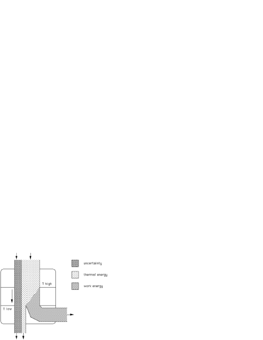
Figure 1: Schematic for a heat engine which brings in heat energy at high temperature and returns heat at low temperature along with energy available for work. One example, applicable to automobile engines, is the lifting of a weighted piston with hot gas which cools on expansion. Another is the storage of available work in plant biomass via photosynthesis of radiation from the sun.

Heat engines as in Fig. 1 are generally defined as steady-state systems which take in heat from a high temperature (e.g. a combustion) reservoir, and return that energy as heat and “ordered energy” to a lower temperature (e.g. ambient) reservoir. Car and steam engines fall into this category, if we allow burning fuel to be considered their source of high temperature heat.

The equations above also work with forms of plant life which take in sunlight (high temperature heat) and store chemical energy (i.e. work) in plant biomass (e.g. in cellulose, carbohydrates, proteins, and fats). In this case, $PdV$ work may be ignored, and $\delta W_{out}-\delta W_{in}$ becomes the change in chemical potential times the number of molecules whose state is changed by solar irradiation. Ecologists refer to organisms that do this as autotrophs (“self-nourishers”) or primary producers Odum (1971).

The exhaust (i.e. low temperature) reservoir for most heat engines is the ambient environment. Refrigerators and electric heat pumps are by comparison heat engines run in reverse, i.e. they take in work and heat from a low temperature reservoir, exhausting it to a warmer ambient. All of the exhausted heat is eventually radiated at around 300K back into space by the earth, letting us see the earth itself as a steady-state heat engine as well.

Solving equations 39 and 40, and assuming that $T_{in}$ is positive, we get the familiar upper limit on energy available for work that a Carnot engine (i.e. an engine whose heat flows out of and into a pair of fixed-temperature reservoirs) can produce:

$$\delta W_{out}\leq\delta Q_{in}\left(1-\frac{T_{out}}{T_{in}}\right)\text{.}$$ (41)

Most real heat engines have efficiencies (conversion fractions) which are beneath this because of irreversibilities during operation.

V.2 Information engines & us

The concepts of thermodynamics have been traditionally honed in systems near or approaching equilibrium, and the entropy of homogeneous systems at equilibrium is an extensive quantity like energy or volume or number of particles. However, the maximum entropy best guess machine is much less restrictive about the kinds of system to which it applies. In particular, uncertainty about the state of a system in general depends not only on what we know about each component of a system, but what we know about the relationship between components.

For example, if 10 white and 10 black marbles are distributed between two drawers A and B, then one has $S=20k\ln 2$, or 20 bits, of uncertainty about the drawer assignment of these marbles (i.e. one true-false question’s worth, or bit, of uncertainty per marble). However, if one is given as true the statement that “marbles in any given drawer are all the same color”, the uncertainty about the drawer assignment of marbles is reduced to $k\ln 2$ or one bit of uncertainty. Even though a bit (literally) of uncertainty remains about the drawer assignment for each individual marble, as before, the total uncertainty has now been decreased by the mutual information in that statement, or

$$M=\sum_{i=1}^{N_{ss}}S_{i}-S_{total}\text{.}$$ (42)

In our example, there are $N_{ss}=20$ subsystems, and this equation shows that $M=20-1=19$ bits of mutual information are contained in the statement quoted above!

Mutual information (e.g. that two spins are correlated, or that two gases have not been well mixed) plays a well-known role in physical systems as well Brilloun (1962); Lloyd (1989); Scully et al. (2003), with recent focus in particular on it’s impact in nucleic acid replication Schneider (1991, 2000) and in quantum computing Wootters and Zurek (1982); Gottesman and Lo (2000). For example, Grosse et al Grosse et al. (2000) use intra-molecule mutual information to distinguish coding and non-coding DNA, instead of autocorrelation functions, because the former does not require mapping symbols to numbers, and because it is sensitive to non-linear and linear dependences. Although constraints of this sort may be incorporated into the maxent formalism (cf. Appendix B), we take the possibility of such correlations into account here by simply modifying equation 13 to read

$$\delta S=\frac{\delta Q_{in}}{T}-\delta M_{internal}+\delta{S_{irr}}\text{.}$$ (43)

This makes the $2^{nd}$ Law relevant to engines whose primary function concerns tasks not explicitly involving changes in energy, such as the job of putting “the kids’ socks in one pile and the parents’ socks in another”, or the challenge of reversible computing. When $\delta M_{internal}$ changes are important, however, note that entropy cannot be considered an extensive quantity like U, V, and N, since the total uncertainty S about the state of a system may be less than the sum of the uncertainties about the state of its constituent parts.

This strategy reflects recent thinking about the energy cost of information in generalizing the Maxwell’s demon problem Bennett (1987). Zurek Zurek (1989) among others suggests that the only requisite cost of recording information about other components in a system is the cost of preparing the blank sheet (or resetting the measuring apparatus prior to recording with it. Moreover, the minimum thermodynamic cost, in energy per unit of correlation information, is simply the ambient temperature $T$.

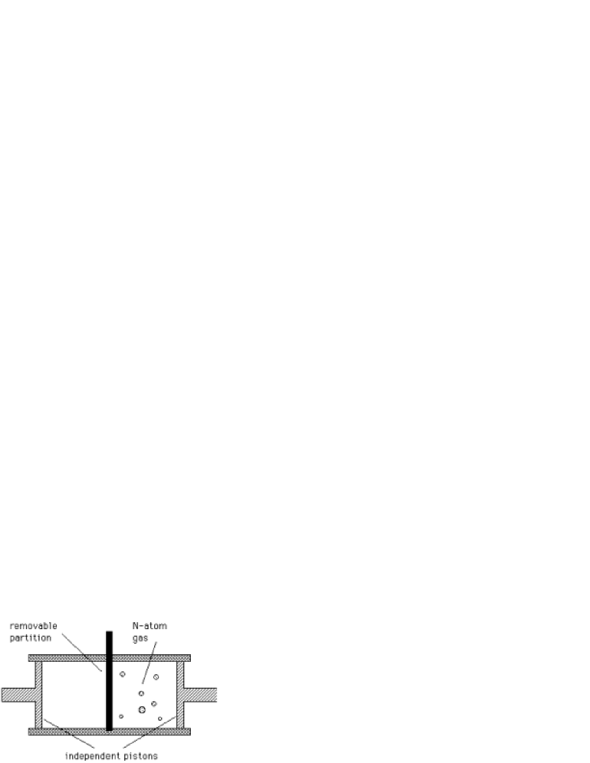
Figure 2: A symmetric bi-partitioned cell for the isothermal compression of an N-atom ideal gas into either its left or right half, perhaps first discussed by Szilard, which serves as a physical system about whose state mutual information is available for a well-defined price in free energy. If one is further provided with some mechanism (e.g. spectroscopic) for reading its state, it may also serve as a mechanically operated single-bit memory. The “setting” process involves removing the barrier between compartments, using the piston on one side to relocate all atoms into the opposite half and then returning the barrier before returning the piston to its original position. The required work is $W_{in}=NkT\ln[2]$. Its reset status may be defined as true if we know that the atoms are located in the right half of the container, and false if we don’t know this to be the case.

A classic example Penrose (1970) of this is the isothermal compressor for an N-atom gas 2, taken for the case when N=1. The system requires thermalization of no less than $kT\ln 2$ of work, in return for a single bit of correlation information concerning the location of the atom. That correlation information in turn can be used subsequently to perform with arbitrarily small energy cost the same task of locating the atom on a desired side, by simply rotating the cylinder by 180 degrees as needed!

The $\Delta M$ term also lets us see the isolated system Second Law (Eqn 10) in a new light. Begin with a system A with $\Omega$ total accessible states, so that uncertainty about A is at most $S[A]=k\ln\Omega$. Then consider an observer B, with sufficient added information about A to limit the number of accessible states to $\Gamma<\Omega$. Observer B therefore has conditional uncertainty about A (see Appendix B) of $S_{B}[A]=k\ln\Gamma$. What we can learn about A by knowing B is then the mutual information $M[A,B]=S[A]+S[B]-S[AB]=S[A]-S_{B}[A]=k\ln\frac{\Omega}{\Gamma}$. If the basic structure of system A from which $\Omega$ was calculated remains intact, then the isolated system $2^{nd}$ Law assertion that observer uncertainty about isolated A can only stay constant or increase (i.e. that $dS_{B}[A]/dt\geq 0$) implies also that the mutual information between two isolated systems (here $M[A,B]$) can only decrease.

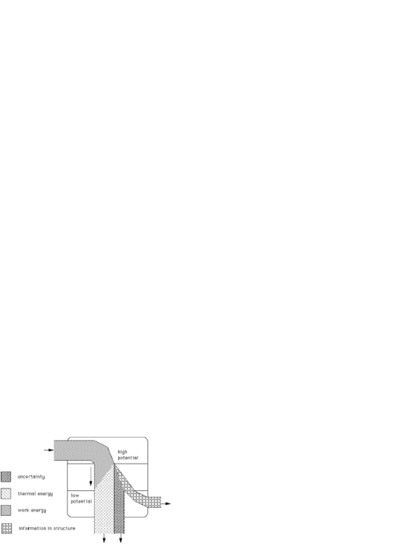
Figure 3: Schematic for an information engine which in the process of thermalizing energy available for work creates mutual information (also called correlation information, information in structure, or negentropy Brilloun (1962)). One example is the isothermal compression of an N-atom gas into the left half of a compartmented container with a vacuum pump, while thermalizing at least $NkT\ln[2]$ of work energy and creating some external record of the occurrence. Another example might be the resetting (erasure) of a used sheet of paper or a molecular template, as a first step in the encoding or replication of a message.

Now we consider steady state engines whose function is to produce mutual information or correlations between two systems, as in Fig 3. These correlations might, for example, be marble collections sorted by color, a faithful copy of a strand of DNA, or dots on a sky map corresponding to the position of stars in the night sky. Our first and second law engine equations (from 39 and 40 with mutual information), become

$$dU=(\delta Q_{out})-(\delta W_{in})=0\text{, and}$$ (44)

$$\delta S=\frac{\delta Q_{out}}{T_{out}}-\delta M_{external}=\delta S_{irr}\geq 0\text{.}$$ (45)

Eliminating $Q_{out}$ from these two equations yields

$$\delta M_{external}\leq\frac{\delta W_{in}}{T}\text{.}$$ (46)

This means that information engines can produce no more mutual information than their energy consumption, divided by their ambient operating temperature. In binary information units, this amounts to producing about 55 bits of information per eV of thermalized work at room temperature, and around 60 bits per eV of energy if operating near the freezing point of water.

Cameras, tape recorders, and copying machines may be considered such information engines, as are forms of life which take in chemical energy available for work from plant biomass, and thermalize that energy at ambient temperature while creating correlations between objects in their environment and their survival needs, and in the form of persistent DNA sequences, behavior redirections, songs, rituals, books, and sets of ideas). Living organisms which do not qualify as heat engines, but which fit this description, are known by ecologists as heterotrophs Odum (1971), a category which includes most non-photosynthetic organisms (including humans).

For a human being consuming $1.3\times 10^{7}$ joules (around 3000 kcal or 7 twinkies) per day, and viewed as an information engine, this implies an upper limit on production of $4\times 10^{27}$ bits of mutual information in our environment per day. (Note: This includes non-coded correlations, like laundry which has been sorted into piles, as well as coded correlations such as a map of the night sky as it looked at 11pm from your backyard.) Much like conservation of mechanical energy limits on speed in roller coaster rides, and Gauss’s law limits on net charge within a volume based on field measurements at the boundaries, this assertion may well stand quite independent of the detailed biochemistry going on inside. Alas some of us, in practice, have trouble putting a one page report of new observations in a file per week! Although individual metazoans in fact bolster the correlation information in their environment on many levels (see the next section), even when unassisted by other sources of energy available for work, it is likely that the above inequality is not a major bottleneck for most.

VI Excitations and codes

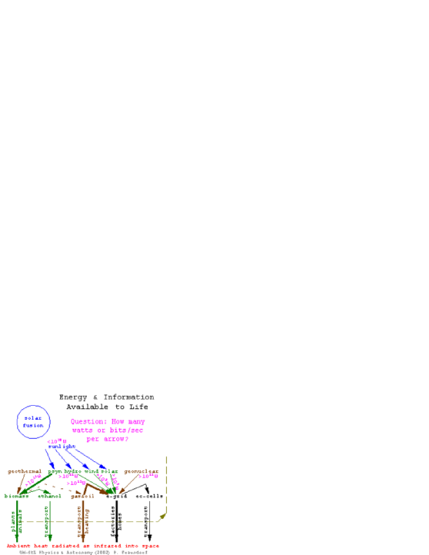
Figure 4: Life’s Energy Flow: The top half represents some of the primary processes involved with energy flow, while the bottom half illustrates significant physical repositories for life’s energies, and paths for conversion of energy from one form to another.

Figure 4 illustrates the flow of energy available to life on earth, much of which began as high temperature radiative heat given off by the sun, subsequently converted to chemical potential energy (heat engine style) in the form of plant biomass Odum (1971). Much work might still be done to quantify these flows Vitousek et al. (1997), since the flow rate through biomass is seldom even considered outside of classes in ecology. For example, many introductory physics texts, and even the world almanac, ignore its size entirely. Hence student projects on the size of these flows, at various times and places, might be interesting and enjoyable. Likewise for projects which examine the involvement of various consumables and activities in the depicted streams e.g. the availability cost of a hot dog, or an aluminum can.

Some of the ”ordered energy” outputs from the heat engines described in Figure 4 are eventually thermalized (e.g. in forest fires or the burning of fossil fuels), but not all of it is irreversibly thermalized. In other words, some of the free energy made available by plants is converted to non-energy related correlations between organism and environment, and some is converted to to internal correlations within living things.

Organism/environment correlations include, for example, cell membranes that separate the contents of one-celled organisms from the fluids surrounding. They differ, depending on the nature of the ambient to which a given organism is adapted. Similarly, the woody trunks of trees don’t merely store chemical energy for later combustion, but instead point in a direction which allows subsequent leaf growth to have better access to the light of the sun.

Figure 5: Life’s Stores of Availability: Horizontal bars represent inward-looking (intra or “yin”) correlations, while vertical bars represent outward-looking (cross-boundary or “yang”) correlations. This breakdown seems to work reasonably well to categorize by domain both the types of correlations that exist, and the kinds of ideas (i.e. memetic replicators) used to help maintain them.

Correlations internal to organisms include catalysts (often amino acid enzymes) which guide the spending of the cell’s energy coin Hoagland and Dodson (1998) (adenosine triphospate molecules) not only toward nourishment and other external goals, but toward it’s use in the process of cell replication. The enzymes themselves are typically constructed from amino acid sequences which fold in solution into secondary and delicate tertiary structures which are crucial to catalyst structure and function.

In fact, information on these correlations within catalyst molecules, resulting in part also in correlations between organisms and their environment, apparently proved so important that a digital means (nucleic acid codes) to store mutual information on these correlations, still in widespread use today, was developed several billion years ago Margulis and Sagan (1986); Ward and Brownlee (2000). Note that the word digital here refers to ways to store mutual information in which bit-wise fidelity of the replication process can be checked after the fact. This is distinct from analog forms of recording, like the storage of images on film, where accuracy on the microscopic scale is lost statistically in the grain structure of the film, as one moves to increasingly smaller size scales.

This ancient invention of digital recording more or less formalized a now long-standing symbiosis between steady-state excitations (in particular organisms which operate in-part by reversibly thermalizing an inward-flowing stream of energy in the form of available work) and replicable codes. This excitation-code symbiosis, of course, involves mutual information managed (stored, replicated, and applied to enzyme manufacture) by biological cells Hoagland and Dodson (1998). Now memetic replicators Dawkins (1989); Blackmore (2000), i.e. ideas which began as sharable patterns stored in the neural nets of animals Dennett (1992); van Schaik et al. (2003), are in the process of going digital McLuhan (1962); Harnad (1991), thus adding a second level to life’s symbiosis with replicators. The unconscious struggle for hegemony over organisms, between these two replicator families, might in a way be seen as a battle between “sword” and “pen” in which (strangely enough) organisms are the spoils of war. At the very least, it seems likely that under some conditions the interests of organisms, and the interests of codes, don’t commute.

Naturally our “organism-centric” vantage point prompts us to miss, at first glance, the way that organisms serve codes in a given process Dawkins (1989). We might sometimes even miss the distinction between “our ideas about the world” (those replicable codes) and “the world itself” (a complex excitation with deep internal correlations) Hofstadter (1985) as though we are in danger of “knowing everything” with a completed map of the universe in our minds Horgan (1996). A closer look at nature, however, reveals that true cloning of internally-correlated excitations (e.g. like qubits Wootters and Zurek (1982)) may be impossible in principle as well as in practice.

A natural way to “illustrate and inventory” the standing crop of correlations associated with life, while recognizing boundaries between replicator-pools as well as simpler physical boundaries (like cell walls and individual spaces), is illustrated in Figure 5. Again, students might find it enjoyable to think about ways to inventory this standing crop of correlations, at various places and times. Although in principle each bar in the figure could be quantified in “bits of standing availability”, neither the means nor the motivation for doing this objectively are clear at this point. However, just picturing qualitatively the state of these correlations and the boundaries with which they associate, as physical elements in the world around, might be worthwhile (cf. Fig 6).

Figure 6: An expanded schematic of some boundaries alone, drawn from Fig 5. This suggests for example that the idea sets for interaction between cultures (i.e. when one has to take into account more than one book in the figure, or meme-pool) may be quite different than those for interactions between heirarchies in a given culture. Guidelines for professionalism in the workplace, and political correctness, as irrelevant as they may seem in the context of one culture, might be evidence of behavior correlations developing along those lines.

VII The natural history of invention

Histories of emergent phenomena, like Marshall McLuhan’s “Gutenberg Galaxy” McLuhan (1962), Konrad Lorenz’ “On Aggression” Lorenz (1966), Margulis & Sagan’s “Microcosmos” Margulis and Sagan (1986), Jared Diamond’s “Guns Germs and Steel” Diamond (1997), David Attenborough’s Special on Birds Attenborough (1997), and Ward & Brownlee’s “Rare Earth” Ward and Brownlee (2000) (in broad strokes at least) simplify when outlined in terms of the two manifestations of generalized availability depicted in Figures 4 and 5: (i) “ordered” or free energy, and (ii) mutual information, respectively. These two themes repeatedly intertwine in a non-repeating drama that involves partnership between replicable codes (which incidentally include the above two concepts), and what physicists might call steady-state excitations busily converting energy and information from one form to another. This history shows potential for providing a neutral perspective, grounded in established physical and logical principles, on numerous important and sometimes contentious issues. By providing context both for such issues and our reactions to them, it might catalyze constructive dialog. It also suggests elements of a natural history, informed to interdisciplinary connections emergent only in the last century.

A larger “timeline of concept-relevance” for ideas might thus, for example, begin with the elemental concepts of:

• dimension (1D, 2D, 3D, 3+1D, n+1D, etc.),

• metric (e.g. Pythagoras’ space & Minkowski’s space-time);

followed by the emergence in our world of manifestations now represented by basic physical concepts like:

• motion, momentum-energy, mass & gravity

• other interactions like charge & electromagnetic force,

• particles, waves, atoms & their associated chemistry,

• heat, an early application of gambling with uncertainty,

• available work and mutual information in physical systems.

Discoveries on earth then lead to the following inventions by one-celled organisms:

• steady-state thermal-to-chemical (i.e. photosynthetic) and chemical to kinetic (i.e. motion) energy conversion,

• energy storage in combustable sugars, and mechanisms for withdrawal (via enzymes) into more easily and universally spendable ATP molecules.

• digital information partnering (trading work for recorded correlations) with highly replicable amino and nucleic acid codes, and thus in a sense the practice (but not yet the idea) of genetic engineering;

• intracellular structures like cell membranes & organelles (symbiotic) and viruses (parasitic),

• chemical and tactile messaging;

• tools like thermal or chemical gradients for locating energy sources, & contact forces for motility;

subsequent inventions by multi-celled plants of:

• intercellular correlations like eukaryotic cells, sexual reproduction & microbe-assisted digestion (symbiotic), or bacterial infections (parasitic),

• differentiated structures like circulatory systems, leaves, stalks, roots, flowers, & shells,

• other intra-organism correlations such as annual/biennial reproductive cycles (symbiotic), or cancerous tissues (parasitic), and

• inter-organism correlations, like ritualized interspecies redirection of behavior by providing animals with fruit and nectar symbiotically, or fake sex parasitically, so as to distribute seeds & pollen,

• messaging via hormone (intra-organism) & exterior design;

• tools like gravity and wind as aids to reproduction;

the invention by animals of:

• information partnering with neural net patterns via sense-mediated action, of limited replicability perhaps greatest in ritualized songs, discovery dances, & warning vocalizations (especially for birds, bees, and mammals),

• intra-organism structures like vertebrae, muscles, brains, eyes with lenses, gills, lungs, hearts, legs & wings,

• intra-species aggression and it’s ritualized redirections Lorenz (1966), including greeting ceremonies, pair bonds & laughter,

• family systems serving inward-looking perspectives with respect to intra-specific gene-pool boundaries, and related correlations like joint-parenting & constructive sibling interactions (e.g. play between kittens),

• political systems serving outward-looking perspectives with respect to intra-specific gene-pool boundaries, and associated correlations such as heirarchy in a wolf pack,

• inter-organism messaging via sound, body language, and interior design (bauer),

• tools like webs, levers, vines, tunnel, dam, wood, & stone;

and finally the invention in human communities of:

• information partnering with highly replicable spoken languages, print, and most recently digital codes,

• available work production & distribution in these forms: food/drink, ritual (monetary), fossil fuel & electrical,

• subsystem repair/augmentation networks like medicine, dentistry, pharmacy, auto repair, & physical therapy,

• redirective elicitors (symbiotic & parasitic) of innate behavior (like eating, procreation & militant enthusiasm) include sports, “mind” chemicals, non-reproductive sex, self-help, psychotherapy, plus artificial colors, flavors, smells & shapes (for food & individuals),

• prediction activities like meteorology, gambling, insurance, digital modeling, investing, polling & quality control,

• evolving pair, family, and heirarchy paradigms with roots in phylogenetic & memetic tradition, like votes, jury, public corporations, church/state separation, free press, merit/goal-based management, human rights,

• belief systems serving inward-looking perspectives with respect to meme-pool boundaries, and related correlations that include religions (symbiotic) & religious colonialism, plus ethnic, cultural, & artistic identities,

• knowledge systems serving outward-looking perspectives with respect to meme-pool boundaries, and related correlations that include professions, “political correctness”, secular colonialism & peer review,

• inter-organism messaging via music, art, writing, printing, teletype, radio, phonograph, telephone, photography, cinema, fingerprint, television, xerography, magnetic tape, bar code, optical disk, pager, sky phone & internet,

• tools like clothes, fire, oven, wheel, ramp, plow, weapons, skyscraper, bike, road, steam/gasoline/electric motors, car, bridge, train, boat, aircraft, match, washing machine, vacuum cleaner, flush toilet, dishwasher, grinders, mirror, glass lens, camera, camcorder, hologram, clock, artificial light, metals, ceramics, concrete, canning, polymers, gear, cam, lock, spring, rope, pulley, block & tackle, zipper, scissors, nail, screw, irrigation, planting & harvesting equipment, wrench, portable drill/saw, end loader, running water, gas & electric heater & drier (for people, food, & clothes), elevator, crane, battery, volt-ohm meter, laser, compass, satellite, global positioning system, gyroscope, autopilot, smoke detector, fridge & air conditioner, X-ray & ultrasound & MRI imaging, tele & micro & endo scopes, spectrometers, semiconductors, transistors, integrated circuits, computers, fiber optics, robotics, and the idea of polymerase chain reaction for nucleic acid sequence replication.

Thus correlations, written in nucleic or amino acid strings, have been developing in symbiosis with microbes since the very early days of our planet. Moreover, sometime since the Cambrian bloom of metazoan body types, and particularly among humans in the past 10,000 years, similar correlations written in memetic codes have been undergoing active development. The latter were of course broadcast not via the sharing of molecules, but by transference between neural nets through metazoan senses via performance, speech, script, and more recently digital means starting with the Phoenician alphabet.

The large number of thermodynamic and information-theoretic processes in this list raises a question about codes that arises often today in context of the human genome project: What gene is responsible for what features of an organism, or conversely what features of an organism does a given nucleic acid sequence “cause”? The same question of course can be asked about memetic codes. Has a given set of ideas been honed via experience with the world around us, via experience with worlds within this boundary or that, or does it offer little by way of connection to the world at all? I hope that we’ve shown here that in any rigorous sense such questions must be considered questions not about the properties of a molecule or a set of words in isolation, but rather questions about delocalized correlations between physical objects (in particular between codes or their phenotypes, and other parts of the world around). Once the context is specified (e.g. the reference state used in equation 36), objective and even quantitative assessments of these correlations may be possible.

Qualitatively, for example, most might agree that the nucleic acid base triplets UAA, UAG, and UGA have evolved as elements of punctuation in the genetic code, there not to correlate with the outside world but to guide the process of transcription into protein, much as the period at the end of this sentence guides the sentence’s transcription into speech. Such punctuation codes are one kind of internal code, developed to guide the replication of codes and their reduction to practice. Other codes have evolved by virtue of (i.e. their survival has been connected in a real-time manner to) the correlations that they affect between an organism and the inanimate world around. Thus a chunk of genetic code might correlate with the thickness to length ratio of a plant’s stem, whose optimum value may depend on wind velocities and topography in the world around. Similarly, a set of ideas for guiding the path of a ship at sea might survive depending on its usefulness in helping the sailors reach their destination, before they run out of supplies.

Some kinds of internal code affect (and are affected by) the way manufacturing is carried out within cells. Others affect the ways cells interact with one another, and yet others affect the way tissues function as a unit, etc., across the levels illustrated in Figure 5. Codes (genetic or memetic) whose survival is predicated primarily on correlations between or internal to lifeforms (rather than specifically between a lifeform and it’s inanimate environment) might be called “we-codes”. Thus for example, many might agree that legal systems provide guidelines (in this case we-memes) for cooperation between more than one genetic subgroup or nuclear family. Clarifying our ideas about the ways that segments of code participate in correlations between the organisms they guide, and other parts of the world, is even more important now that genetic codes are being transribed by humans into memetic form.

Examining any given correlation from this list quantitatively (cf. Appendix B) may or may not be meaningful. However, the list does make it easy to see why thermodynamic metaphors (e.g. as recently pointed out by a social-science student in a physics class here) seem relevant to processes found in even the most complex social systems, including economic systems that involve money (a ritually-conserved quantity designed for portability). Thus management of energy flows through various forms of available work, ways to thermalize that energy reversibly so as to create and preserve correlations between and within organisms and their environment, and the storage of information in increasingly more replicable forms, are central and recurring parts of life’s adventure.

VIII Net surprisal & the unexpected

Entropy, a measure of expected or average surprisal, has been important in thermodynamics since the work of Clausius in 1865, although its firm connection to information measures is more recent. Net surprisals, defined as a difference in average surprisals between one state of information and another (the second being often some reference or equilibrium state), were initially referred to by Gibbs in 1875 as availabilities Knuth (1966). Generalized availabilities, negative logarithms of the partition function as shown above, are deeply rooted in the mathematics of statistical inference, and increasingly recognized for their connection to both free energy Evans (1969); Tribus and McIrvine (1971) and complexity Morowitz (1968). Lloyd’s measure of complexity via depth is in the same category Lloyd (1990).

Although we stop with the discussion of net surprisals here, it is difficult to resist pointing out that lifeforms, as information engines in symbiosis with codes which survive by replication, have a vested interest in being able to distinguish alternatives with high net surprisal relative to an expected ambient (i.e. with respect to what is common). The noble passions ala Fig 5, e.g. for being a good friend/mentor, sibling/parent, citizen/leader, believer/cleric, and witness/scholar, may be considered evidence of interest in recognizing net surprisal.

Corollary symptoms of preoccupation with recognizing high net surprisal include: (a) the positive importance in human culture of attributes like special, unique, or rare; (b) the human appetite for variety, pleasant surprises, and even gambling; (c) the importance of special recognition throughout life, including the need for attention as a youngster and the need to signify, have great “discretionary power”, or be famous as an adult; (d) the importance of humor, and the discovery of novel, fortuitous, and/or surprising connections in our language and behavior as a kind of “dessert” for us information processors at the end of a long day’s work; (e) the use in the vernacular of adjectives like “heated”, “hot”, and “steamed” for situations in which action dominates thought (e.g. high eV/bit), and adjectives like “cool” for situations in which information dominates by comparison; and (f) of course the desire to see the genetic and memetic codes, that we’ve had a hand in designing, fare well with challenges posed by their environment in days ahead.

IX Conclusions

Statistical physics is perhaps the most quantitative tool available for the generalist, in that it allows one with meager information to make rigorous assertions that a subset of outcomes are going to be impossible in practice. Perpetual motion machines Penrose (1970) are the classic example. Although the calculation methods, and some of the examples used above, are old, the problems they can address are contemporary.

As tools in the “science of the possible” these methods can be used to show (for example) that reversible methods for converting high temperature heat to low temperature heat for home heating could reduce the energy cost of heating by an order of magnitude Silver (1981); Jaynes (1991), and that going to the store to buy a package of automobile seeds is not an inconceivable alternative for our descendants a century from now Drexler (1986). Awareness of mutual information is crucial to our understanding of both quantum computers of the future Gottesman and Lo (2000), and the molecular machines for replicating nucleic acid sequences which keep us going today Schneider (2000).

Concerning the information theory paradigm itself, Amnon Katz said in the preface to his 1967 book Katz (1967) that writing a book on the information theory approach to statistical physics was worthwhile to him primarily because it provides a coherent overview for the novice. He said that his book found little favor with the experts in statistical mechanics, because they already knew how to pose questions and get answers. Part of the disinterest in a new way to look at things on the part of experts Gopal (1974) was likely paradigm paralysis of the same sort that prompted Swiss watchmakers in the late 1960’s to discredit as uninteresting, and to eventually give away, their own invention of the quartz-movement watch along with most of their market share in the watchmaking industry Barker (1986).

Now, a half-century later, the pervasive influence of the paradigm shift on mid-level physics texts, and the experimental impact of mutual information in molecular biology and nano-computing research, has left skeptics (even if they are legitimately tired of hand-waving metaphors) with little to hang onto except the large size of Avogadro’s number, which makes uncertainty increases associated with heat flow tens of orders of magnitude larger than those associated with the traditional objects of gambling theory Lambert (1999). The good news here is that the paradigm shift offers additional food for thought to students not majoring in physics (especially those involved in the code-based sciences). Of course it is in part the responsibilty of physicists to provide such students, in an introductory course, with physical insight into quantitative ways for putting these tools to use.

Appendix A Multiple choice maxent

Suppose we wish to determine the “state” of a population of individuals with respect to the way they will respond to the questions on an $N$ question, $m$ choice multiple-choice test. The only information that we have, however, is the average number of correct answers $\kappa\equiv\left<j\right>$ by members of that population.

Let’s examine the situation more closely. There are $m$ ways to answer each question, so there are $m^{N}$ ways to respond to the test as a whole. For each possible number of correct answers $j\epsilon\{0,N\}$ there are

$$\text{number of states}=\frac{N!}{j!(N-j)!}(m-1)^{N-j}\equiv d_{j}\text{.}$$ (47)

The function $d_{j}$ is called the density of states. Using it, we can write the results of the entropy maximization from equations 17, 18, and 19, respectively, as

$$p_{j}=\frac{e^{-\lambda j}}{Z}\text{; }Z=\sum_{j=0}^{N}d_{j}e^{-\lambda j}\text{; }\frac{S}{k}=\ln Z+\lambda\kappa\text{.}$$ (48)

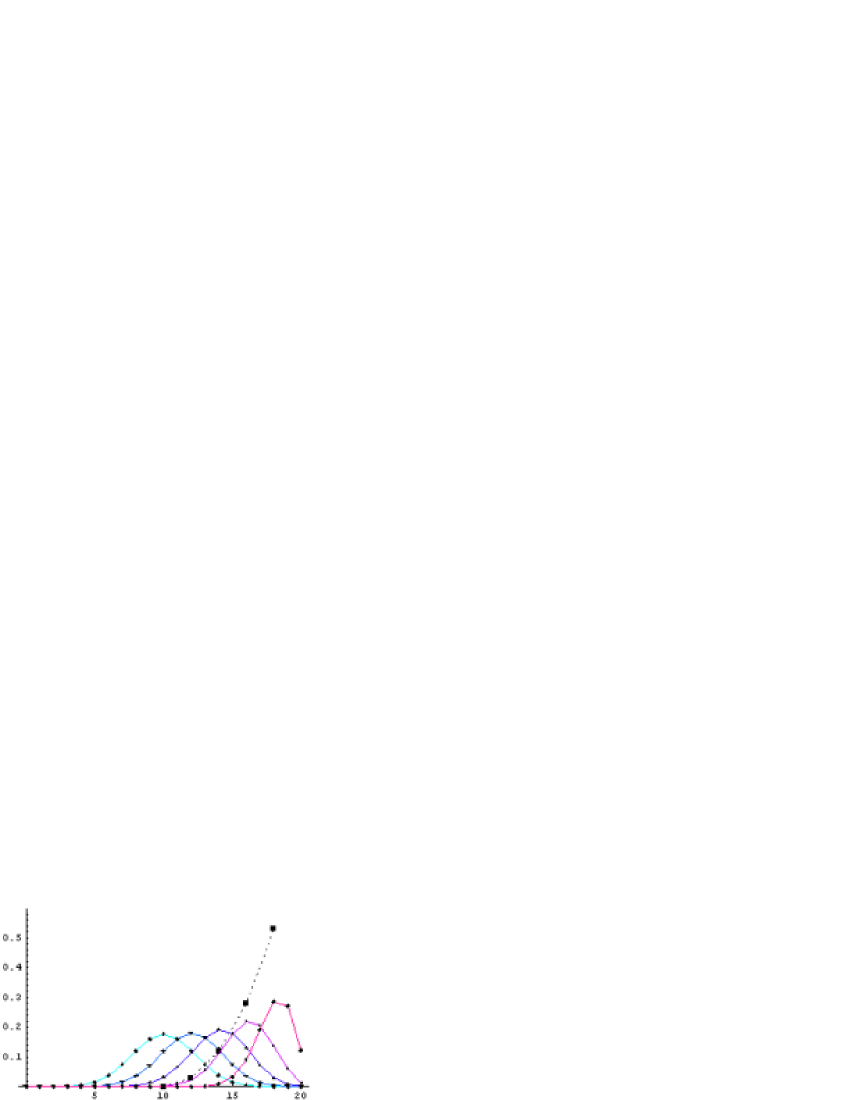
Figure 7: Guessed fraction of students versus the number of correct answers out of 20 questions, when the average grade for the class is 10, 12, 14, 16 and 18. The dashed line is the net surprisal (in bits per question) of the distribution with given average, relative to that expected for 20 randomly answered true-false questions.

The value of $\lambda$ is found by solving the implicit equation $\kappa\equiv\sum_{j=0}^{N}jd_{j}p_{j}$. The result is $\lambda=-\ln\frac{(m-1)\kappa}{N-\kappa}$, so that $Z={\left(\frac{N(m-1)}{N-\kappa}\right)}^{N}$, $S=k\ln\frac{N^{N}\left({m-1}\right)^{N-\kappa}}{\kappa^{\kappa}\left({N-\kappa}\right)^{N-\kappa}}$, and

$$d_{j}p_{j}=\frac{N!}{j!(N-j)!}{\left(\frac{\kappa}{N}\right)}^{j}{\left(\frac{N-\kappa}{N}\right)}^{N-j}\text{.}$$ (49)

When the $d_{j}p_{j}$ are plotted as a function of $j$ for a given value of $\kappa$ (cf. Fig 7), one gets the binomial distribution. This in turn for large N and values of $\kappa$ not too large or small may be approximated by the continuous Gauusian distribution or Bell curve. When $N$ is large but the $\kappa$ is very small by comparison, it reduces to the Poisson distribution, useful for predicting random but unlikely events like the distribution of meteor impacts. The net surprisal per question (dotted line in Fig 7) quantifies the amount of mutual information about course material (relative to random answers on a true-false test) evidenced by students with a given mean score. This net surprisal measure ($I_{net}=kN\ln m-S$) can help teachers take into account the fact that a score of N/m correct, on an m-choice N-question test, provides zero evidence of student learning since random guesses would on average yield the same result.

The entropy of the state distribution $S$ also quantifies our uncertainty about the response of any particular member of the population to the test, given only the population average grade. There is an alternative way to look at it as well. Suppose there was some physical process operating which acted only to hold the average grade at the specified value, but otherwise had no effect on the probability distribution. If that were the only physical process determining the outcome of the test, then we might expect the actual spread in test responses to agree with the distribution of responses predicted by equation 48, which guesses based only the measured value for $\kappa$. Thus even given detailed information on the set of responses to the test, it would help little in decreasing our uncertainty when trying to predict responses because the constraint on $\kappa$ was the only physical process constraining the distribution.

This is more than idle speculation. Indeed the main control variable in educational testing is often the “difficulty” of the questions, and actual test responses for a given average grade do tend to follow the distribution predicted in equation 48. Failure of this to occur is thus evidence for other constraints operating (e.g. the presence of two populations of students). By the same token, agreement between the predicted distribution and the actual one cannot, however, be taken as evidence that no other physical principles are active in the system, only that the results of the test probably tell us little about them.

In the foregoing example, the response of a population sample to a test was classified into a set of “microstates”. The uncertainty about the response given only information about the average grade was shown to agree with the spread in measured values, from which it was inferred that the major physical constraint acting on the response distribution was in effect one which determined the average value. In a more general sense when we consider all of the physical microstates accessible to a given system, the physical entropy of that system is defined as the uncertainty calculated when all externally detectable constraints on the state distribution are used as constraints in the maxent calculation used. It is thus the minimum uncertainty possible, based on all of the “mutual information” about the system available to the world outside.

Appendix B Mutual information basics

A discussion of correlated subsystems which, between themselves, house mutual information must begin with a definition of subsystems. Such subsystems are variously defined, for example, as individual particles, as collections of particles, as individual states (which may or may not be occupied with particles), and as regions or control volumes in and out of which energy and mass might flow. Our earlier distinction between a steady state engine and its environment, as well as the molecule, cell, tissue, metazoan, gene-pool and meme-pool boundaries discussed in section VI, also fall in this category.

Even the isolated-system second law itself must first separate the world into observed-system and observer, because as we mentioned earlier it also is an assertion about the time evolution of mutual information, namely: The correlation information that an observed physical system has with an environment from which it is isolated will not decrease with time, and will likely increase since information available to the environment needed to model propagation of the isolated system through time may fall short.

Once some hopefully useful boundaries for the subsystems of interest in a given problem have been defined, a set of $N_{ss}$-subsystem joint probabilities can be defined. For $N_{ss}=2$, joint probabilities $p[ij]\geq 0$ obey $\sum_{i}\sum_{j}p[ij]=1$. Here the $i$ indices run over all possible states for subsystem I, while the $j$ indices run over all possible states for subsystem J. From the joint probabilities one can calculate marginal probabilities like $p[i]\equiv\sum_{j}p[ij]$, which ignore the state of other subsystems, and conditional probabilities like $p_{i}[j]\equiv\frac{p[ij]}{p[i]}$ associated with a specific state of one subsystem (here the ith state of subsystem I). From these probabilities then values for joint entropy $S[IJ]/k\equiv\left<-\ln p[ij]\right>$, marginal entropies like $S[I]/k\equiv\left<-\ln p[i]\right>$ and conditional entropies like $S_{I}[J]/k\equiv\left<-\ln p_{i}[j]\right>$ follow immediately. Mutual or correlation information between systems I and J, denoted here as $M[I,J]$ and defined by equation 42 as the sum of marginal entropies $S[I]+S[J]$ minus the joint entropy $S[IJ]$, thus becomes

$$M[I,J]=-k\sum_{i}{\sum_{j}p[ij]}\ln\frac{p[i]p[j]}{p[ij]}\geq 0\text{.}$$ (50)

Thus from equation 36 it appears that mutual information is simply the net surprisal that follows upon learning that systems (here I and J) are not independent.

Examples of correlated subsystem pairs include photon or electron pairs with opposite but unknown spins, a single strand of messenger RNA and the sequence of nucleotides in the gene from which it was copied, a manuscript and a copy of that manuscript created with a xerox machine (or a video camera), your understanding of a subject before being given a test and the answer key used by the teacher to grade that test (hopefully), enzymes and coenzymes with site specificity, tissue sets treated as friendly by your immune system, metazoans who developed from the same genetic blueprints (e.g. identical twins), families that share similar values, and cities which occupy similar niches in different cultures (e.g. sister cities). As you might imagine this list of subsystem pairs is incomplete, and many of the quantities listed remain difficult to quantify.

With increasing $N_{ss}$, the number of marginal and conditional entropies increases rapidly, and many new mutual information terms (all positive) emerge as well. For example, when $N_{ss}=3$, marginal probabilities exist which ignore either one or two sub-systems (e.g. like $p[ij]\equiv\sum_{k}p[ijk]$ and $p[i]\equiv\sum_{j}\sum_{k}p[ijk]$). Similarly conditional probabilities can specify the state of one or two sub-systems. These all give rise to analogous marginal and conditional entropies. Lastly, a set of seven mutual information terms can be calculated: the joint correlation $M[I,J,K]\equiv S[I]+S[J]+S[K]-S[IJK]$, three one-on-two terms like $M[I,JK]\equiv S[I]+S[JK]-S[IJK]$, and three one-on-one terms like $M[I,J]\equiv S[I]+S[J]-S[IJ]$.

These mutual information terms all have positive values which are independent of argument ordering, e.g. $M[I,J]=M[J,I]$. One useful identity is $M[I,J,K]=M[I,JK]+M[J,K]$, which in words says that “the joint mutual information of systems I, J and K is the correlation information between system I and system JK, plus that between systems J and K”. Another relationship that we conjecture here is $M[I,JK]\geq M[I,J]$, or in other words:“System I and system JK have at least as much in common as do systems I and J alone”.

The maxent formalism, of course, automatically estimates joint probabilities, from which all of these quantities follow. Figuring out how to constrain the maximization with knowledge of mutual information between subsystems is therefore the primary challenge in adapting it to such problems.