Resistive magnetohydrodynamic equilibria in a torus

Abstract

It was recently demonstrated that static, resistive, magnetohydrodynamic equilibria, in the presence of spatially-uniform electrical conductivity, do not exist in a torus under a standard set of assumed symmetries and boundary conditions. The difficulty, which goes away in the “periodic straight cylinder approximation,” is associated with the necessarily non-vanishing character of the curl of the Lorentz force, ${\bf j}\mbox{\boldmath$\times$}{\bf B}$. Here, we ask if there exists a spatial profile of electrical conductivity that permits the existence of zero-flow, axisymmetric resistive equilibria in a torus, and answer the question in the affirmative. However, the physical properties of the conductivity profile are unusual (the conductivity cannot be constant on a magnetic surface, for example) and whether such equilibria are to be considered physically possible remains an open question.

I INTRODUCTION

Discussions of the magnetic confinement of plasmas and their stability usually begin with the subject of magnetohydrodynamic (MHD) equilibria. [1, 2] In the present generation of devices, dominated by the tokamak concept, the magnetofluids usually carry currents and contain strong dc magnetic fields whose sources are in external coils.

Since the earliest days of fusion research, the various MHD equilibria have been treated as ideal. They are assumed to have infinite electrical conductivity and no flow, so that Ohm’s law,

$${\bf E}+{\bf v}\mbox{\boldmath$\times$}{\bf B}={\bf j}/\sigma,$$ (1)

is satisfied by taking all three terms equal to zero. Here, ${\bf E}$ is the electric field, ${\bf v}$ is the fluid velocity, ${\bf j}$ is the electrical current density, and $\sigma$ is the electrical conductivity, allowed to become infinite. In familiar “Alfvenic” dimensionless units, the curl of the magnetic field ${\bf B}$ is just ${\bf j}$, and of course, the divergences of ${\bf B}$ and ${\bf j}$ are zero. In the limit of infinite conductivity, the sharp connection that must exist between ${\bf E}$ and ${\bf j}$ for large but finite conductivity is, of course, destroyed. There have been attempts to reintroduce the effects of finite conductivity (e.g., see Grad and Hogan [3]), but these attempts are in our opinion not a satisfactory resolution; too many possibilities are raised to be able to deal with any one of them conclusively.

With the infinite conductivity assumption, the only remaining MHD requirement for equilibrium is one of mechanical force balance, with the local Lorentz force ${\bf j}\mbox{\boldmath$\times$}{\bf B}$ taken equal to $\nabla p$, the mechanical pressure gradient. Such ideal equilibria are plentiful [1, 2] and are not constrained by the Ohm’s law. The Grad-Shafranov formulation [1, 2, 4, 5] then provides a framework in which axisymmetric, toroidal ideal equilibria can be calculated.

Investigating the stability of such ideal equilibria can be a lengthy undertaking. This is particularly true when the program includes investigating the various “resistive instabilities” that the ideal equilibria may be thought heir to. Aside from the questions of consistency raised by ignoring resistive terms when constructing the equilibria, but then including them in the linear stability analysis, the possibilities for uncovering new variants of non-ideal, normal modes growing about ideal steady states can seem almost limitless.

The purpose of this paper is to re-open the subject of zero-flow MHD steady states by considering the implications of retaining Eq. (1) with finite $\sigma$. Attention will be confined to axisymmetric steady states with zero flow (${\bf v}=0$) in the simplest toroidal geometry. A previous note by Montgomery and Shan [6] reported a proof of a somewhat unanticipated result: no such equilibria exist for the case of spatially uniform $\sigma$. Here, we inquire into what kinds of spatial dependences of the conductivity $\sigma$ will permit axisymmetric, toroidal steady states without flow. We do not answer the question of how such conductivity profiles might occur, or indeed whether they are to be expected on physical grounds.

The hydrodynamic precedent suggests the need for such inquiries, as illustrated by plane shear flows such as pipe flow, plane Poiseuille flow, or flow around obstacles (e.g., see Acheson [7]). In the case of pipe flow, for example, a uniform pressure gradient balances the axial viscous body force in the steady state. In the “ideal” limit, both may be allowed to go to zero proportionately, but the connection between them must not be lost, or what was a well-determined (parabolic) velocity profile may become anything at all; any axial velocity dependence upon radius is an acceptable steady state, clearly a nonsensical conclusion. Yet the stability of each one of these possible profiles could be investigated ad infinitum.

It is perhaps worth remarking that in the absence of flow velocity, the situation described here is one of classical resistive magnetostatics, and may be treated by standard methods borrowed from electricity and magnetism textbooks. One can say that until a magnetofluid begins to flow, it does not know whether it is a solid piece of metal with a particular spatially-dependent electrical conductivity or a plasma. Once the requirement of balancing the Lorentz force against a scalar pressure gradient is met, none of the additional approximations or assumptions of magnetohydrodynamics per se need to be used for this problem.

We also mention that recently, Bates and Lewis [8] have developed mathematical machinery for treating toroidal equilibrium profiles in true toroidal coordinates. They were able to substantiate the result of Montgomery and Shan [6] in considerably more detail.

It is important that the point of view adopted here be stated clearly. We believe the full set of time-independent MHD equations, including resistivity, velocity fields, tensor transport coefficients, and realistic boundary conditions, are far too difficult to solve at this moment. This is the reason that nearly all MHD equilibrium theory has been ideal, and has omitted these effects, even when it has been asserted that ”resistive instabilities” were being calculated. We are interested in moving as far as we can to remove the above restrictions, but we are also interested in doing so only by exhibiting explicit solutions to whatever problem is undertaken. We are fully aware of the desirability of including all of the complications. Here, only one is included: finite resistivity. It is a new result that there exist finite-resistivity toroidal MHD equilibria without flow, which, in many ways, do not look vastly different from ideal equilibria. How these states that are exhibited here relate to more general toroidal solutions with flow and the other possible complications is a separate, and much harder, question.

This paper is organized as follows. In Sec. II, we ask and answer the question of what kinds of spatial profiles of scalar conductivity will permit axisymmetric toroidal equilibria in the presence of a stationary, toroidal inductive electric field. A partial differential equation is developed which can be thought of as replacing the Grad-Shafranov equation. In Sec. III, particular cases are worked out in detail. Implications are discussed in Sec. IV, along with questions about possible developments and extensions of the theory.

II THE FINITE-CONDUCTIVITY DIFFERENTIAL EQUATION

In toroidal geometry (in contrast to the “straight cylinder” approximation [9, 10, 11, 12]), the steady-state Maxwell equation, $\nabla\mbox{\boldmath$\times$}{\bf E}=0$, has non-trivial implications for the zero-flow Ohm’s law. We use cylindrical coordinates $(r,\varphi,z)$ whose associated unit basis vectors are $({\bf\hat{e}}_{r},{\bf\hat{e}}_{\varphi},{\bf\hat{e}}_{z})$. The $z$ axis is the axis of symmetry of the torus, and $z=0$ is the midplane. Axisymmetry implies that the components of each vector field are independent of the azimuthal coordinate $\varphi$. The center line of the torus will be taken to be the circle $r=r_{0},z=0$. The toroidal cross section will be specified by giving some bounding curve in the $r,z$ plane that encloses this center line. We will choose a specific shape when illustrating the results of the formalism. The wall of the container will be idealized as a rigid conductor coated with a thin layer of insulating dielectric. We do not consider the slits and slots that are necessary in any conducting boundary to permit the driving (toroidal) electric field to penetrate and drive the toroidal current.

The electric field ${\bf E}=E_{\varphi}{\bf\hat{e}}_{\varphi}$ will be assumed to result from a time-proportional magnetic flux ($z$ direction) which is confined to an axisymmetric iron core whose axis coincides with the $z$-axis and which lies entirely inside the “hole in the doughnut” of the torus. The iron core is assumed to be very long, so the inductive electric field it produces in response to a magnetic flux that increases linearly with time is independent of the $z$-coordinate. Faraday’s law then implies that $E_{\varphi}(r)=E_{0}r_{0}/r$ only, where $E_{0}$ is the value of the electric field at $r=r_{0}$. This is a highly simplified cartoon of a tokamak geometry, and it is not difficult to think of ways in which it could be made more realistic. For example, in a more refined model ${\bf E}$ might contain the gradient of a function of both $r$ and $z$ that obeys Laplace’s equation. We do not consider here the possibility of a poloidal current density that could result from a tensor conductivity.

The fact that ${\bf E}$ has this form, which is dictated by Maxwell’s equations, has implications for ${\bf j}=\sigma{\bf}{\bf E}$: for a scalar conductivity $\sigma$, ${\bf j}$ must also point in the $\varphi$ direction. We shall assume that $\sigma$ is a function, as yet unspecified, of both $r$ and $z$.

The magnetic field consists of a toroidal part $(B_{0}r_{0}/r){\bf\hat{e}}_{\varphi}$, and a poloidal part ${\bf B}_{p}(r,z)$ whose curl must be ${\bf j}$:

$${\bf B}=\frac{B_{0}r_{0}}{r}{\bf\hat{e}}_{\varphi}+{\bf B}_{p}(r,z).$$ (2)

$B_{0}$ is the strength of the toroidal field at $r=r_{0}$; it is supported by external poloidal windings around the torus. The source for ${\bf B}_{p}$ is ${\bf j}$, so that

$$\nabla\mbox{\boldmath$\times$}{\bf B}_{p}={\bf j}=\frac{\sigma E_{0}r_{0}}{r}\,{\bf\hat{e}}_{\varphi}.$$ (3)

The boundary condition on the magnetic field is ${\bf B}\cdot{\bf\hat{n}}=0$, where ${\bf\hat{n}}$ is the unit normal to the surface of the torus. Thus the magnetic field lines will be assumed to be confined to the torus, and we do not inquire into the necessary external “vertical field,” or other current distribution required to satisfy boundary conditions on ${\bf B}$ outside the torus.

In addition to solving Eq. (3) subject to the boundary condition, the remaining part of the problem is guaranteeing the force balance, $\nabla p={\bf j}\mbox{\boldmath$\times$}{\bf B}$. This can be done by taking the divergence of this relation and solving the resulting Poisson equation for $p$. In order for there to exist such a solution, it is necessary that

$$\nabla\mbox{\boldmath$\times$}\left({\bf j}\mbox{\boldmath$\times$}{\bf B}\right)=\nabla\mbox{\boldmath$\times$}\left(j_{\varphi}{\bf\hat{e}}_{\varphi}\mbox{\boldmath$\times$}{\bf B}_{p}\right)=0.$$ (4)

For uniform $\sigma$, it is not possible [6] to satisfy Eq. (4). In the present circumstance, the question is asked: “What profiles of $\sigma(r,z)$ make it possible to satisfy Eq. (4) and then ultimately, Eq. (3)?” Note that we are not necessarily assuming either incompressibility or uniform mass density.

If we derive ${\bf B}_{p}$ from a vector potential, ${\bf B}_{p}=\nabla\mbox{\boldmath$\times$}A_{\varphi}(r,z){\bf\hat{e}}_{\varphi}$, and compute $\nabla\mbox{\boldmath$\times$}({\bf j}\mbox{\boldmath$\times$}{\bf B})$, we see that Eq. (4) is equivalent to

$${\bf B}_{p}\cdot\nabla\left(j_{\varphi}/r\right)=\left[-\frac{\partial A_{\varphi}}{\partial z}\frac{\partial}{\partial r}+\frac{1}{r}\frac{\partial}{\partial r}(rA_{\varphi})\frac{\partial}{\partial z}\right]\frac{j_{\varphi}}{r}=0.$$ (5)

The general solution of Eq. (5) is $j_{\varphi}/r=f(rA_{\varphi})$, where $f$ is any differentiable function of its argument. The only remaining equation to satisfy is Eq. (3), or $\nabla\mbox{\boldmath$\times$}\nabla\mbox{\boldmath$\times$}A_{\varphi}{\bf\hat{e}}_{\varphi}=j_{\varphi}{\bf\hat{e}}_{\varphi}$, which can be written as

$$\frac{\partial^{2}A_{\varphi}}{\partial r^{2}}+\frac{1}{r}\frac{\partial A_{\varphi}}{\partial r}-\frac{A_{\varphi}}{r^{2}}+\frac{\partial^{2}A_{\varphi}}{\partial z^{2}}=-rf(rA_{\varphi}).$$ (6)

Eq. (6) is structurally similar to the Grad-Shafranov equation; any choice of $f$ will lead to a partial differential equation for $A_{\varphi}(r,z)$ which must be solved subject to boundary conditions. However, a new restriction on the spatial conductivity is implied. Namely, the toroidal current density $rf(rA_{\varphi})$ must determine $\sigma$ by

$$rf(rA_{\varphi})=\frac{E_{0}r_{0}\,\sigma(r,z)}{r}\,.$$ (7)

The right hand side of Eq. (7) must always be positive, but seems otherwise unrestricted. In terms of the conventional poloidal flux function $\psi=rA_{\varphi}$, the conductivity $\sigma$ is seen not to be a “flux function.” That is, it is not constant on a surface of constant $\psi$, since it is the square of $r$ times a function of $\psi$. It is often thought that $\sigma$ should be constant on surfaces of constant $\psi$, since it depends strongly on temperature and flux surfaces are often imagined to be surfaces of constant temperature.

For a specific form of the function $f$, the problem of finding the solution to Eq. (6) is straightforward; justifying the spatial dependence of the conductivity implied by Eq. (7), however, is not.

We pass now to the consideration of some special choices of the function $f$ and their consequences.

III TWO EXAMPLES

We do not presently inquire into the physical basis of any possible choice of $f(rA_{\varphi})$, such as, say, a maximum-entropy or minimum-energy choice. Rather, we select two examples largely on the basis of algebraic simplicity, and also choose a toroidal cross section for which the equation becomes separable and the boundary conditions tractable. Even then, both cases exhibit some complexity.

A The choice f = constant

The simplest choice is to set $f$ equal to a positive constant $\lambda>0$, making the toroidal current density $j_{\varphi}$ proportional to $r$ and independent of $z$. It should be noted that this $r$-proportionality (for vorticity) was found useful by Norbury [13] in a study of vortex rings. These were ideal vortex rings, however, and required no external agency to maintain them against dissipation. This makes the conductivity $\sigma$ vary as the square of $r$, increasing toward the “outboard” side of the torus.

Eq. (6), with $f=\lambda$, may be solved by first noting that it has become a linear, inhomogeneous, partial differential equation, the general solution to which is any particular solution plus the most general solution of the associated homogeneous equation. A particular solution is $A_{\varphi}=-\lambda r^{3}/8$. The remaining homogeneous equation is the equation for a vacuum poloidal axisymmetric magnetic field. An easy way to find this vacuum field is to rewrite it in terms of a magnetic scalar potential $\Phi$ that obeys Laplace’s equation:

$${\bf B}_{p}=\nabla\mbox{\boldmath$\times$}A_{\varphi}{\bf\hat{e}}_{\varphi}=-\frac{\lambda}{8}\,\nabla\mbox{\boldmath$\times$}r^{3}{\bf\hat{e}}_{\varphi}+\nabla\Phi,$$ (8)

where $\nabla^{2}\Phi=0$. The boundary condition is ${\bf B}_{p}\cdot{\bf\hat{n}}=0$ over the toroidal surface.

Satisfying this boundary condition over a curved surface is a difficult task; [6] see, however, Bates and Lewis.[8] For illustrative purposes, we consider a torus with a rectangular cross section. We assume the toroidal boundaries to lie at $z=\pm L$, and at $r=r_{-}$ and $r=r_{+}$, where $r_{-}<r<r_{+}$. The vanishing of the normal component of ${\bf B}_{\varphi}$ at these boundaries amounts to demanding that

$$\frac{\partial\Phi}{\partial r}=0\,,\hskip 28.90755pt{\rm at}\hskip 14.45377ptr=r_{-},\;r_{+}\,$$ (10)

$$\frac{\partial\Phi}{\partial z}=\frac{\lambda r^{2}}{2}\,,\hskip 14.45377pt{\rm at}\hskip 14.45377ptz=\pm L\,.\;\;\;\;$$ (11)

The general solution of $\nabla^{2}\Phi=0$ for $\Phi$ can be written as

$$\Phi=C_{0}z+\sum_{k}\left[C_{k}J_{0}(kr)+D_{k}Y_{0}(kr)\right]\sinh\left(kz+\alpha_{k}\right),$$ (12)

where $J_{0}$ and $Y_{0}$ are the usual Bessel and Weber functions, respectively, and $C_{0}$, $C_{k}$, $D_{k}$, and $\alpha_{k}$ are arbitrary constants. The values of $k$ remain to be determined.

Eq. (10) is satisfied by requiring that

$$C_{k}J_{0}^{\prime}(kr_{-})+D_{k}Y_{0}^{\prime}(kr_{-}) = 0\,,$$ (13)

$$C_{k}J_{0}^{\prime}(kr_{+})+D_{k}Y_{0}^{\prime}(kr_{+}) = 0\,,$$ (14)

where the primes indicate differentiation with respect to the arguments of the functions. Eqs. (13) and (14) can only be solved consistently for $C_{k}$ and $D_{k}$ if the determinant

$${\cal D}\equiv J_{0}^{\prime}(kr_{-})Y_{0}^{\prime}(kr_{+})-J_{0}^{\prime}(kr_{+})Y_{0}^{\prime}(kr_{-})$$

vanishes. For an infinite sequence of $k$-values, with each $k$ corresponding to a particular zero of ${\cal D}$ for given values of $r_{-}$ and $r_{+}$, general Sturm-Liouville theory tells us that the functions

$$\phi_{k}\equiv\epsilon_{k}\left[J_{0}(kr)+(D_{k}/C_{k})\,Y_{0}(kr)\right],$$ (15)

form a complete orthonormal set on the interval $r_{-}<r<r_{+}$. The $\epsilon_{k}$ are real constants chosen to normalize the $\phi_{k}$:

$$\int_{r_{-}}^{r_{+}}\phi_{k_{1}}\phi_{k_{2}}r\,dr=\delta_{k_{1},\,k_{2}}\,.$$ (16)

The $z$-boundary conditions can both be satisfied by choosing the $\alpha_{k}=0$ for all $k$. The requirement is

$$\tilde{C}_{0}\,\phi_{0}+\sum_{k}k\,\tilde{C}_{k}\,\phi_{k}(r)\,\cosh kL=\frac{\lambda r^{2}}{2}\,,$$ (17)

where $\phi_{0}=\epsilon_{0}$ is a constant. This can be achieved if the expansion coefficients $\tilde{C}_{k}$ are chosen according to

$$\tilde{C}_{0}=\frac{\lambda\epsilon_{0}}{2}\int_{r_{-}}^{r_{+}}r^{3}\,dr\,,$$ (18)

for $k=0$, and

$$\tilde{C}_{k}=\frac{\lambda}{2}\int_{r_{-}}^{r_{+}}\phi_{k}(r)r^{3}\,dr/\left[k\cosh kL\right],$$ (19)

for $k\neq 0$. The full solution for ${\bf B}_{p}$ is then given by Eq. (8), with

$$\Phi=\tilde{C}_{0}\,\phi_{0}\,z+\sum_{k}\tilde{C}_{k}\,\phi_{k}(r)\,\sinh(kz)\,.$$ (20)

In order to determine the allowed values of $k$ in this problem, the zeros of the determinant ${\cal D}$ must be found. The function ${\cal D}$ is an oscillating function of $k$ that intersects the positive $k$-axis an infinite number of times. Using standard numerical techniques, the intersections can be computed for specified values of $r_{-}$ and $r_{+}$, and in this way the discrete spectrum of the permitted $k$ values determined. For each $k$, we may calculate $C_{k}/D_{k}$. The results for the $k$ values, the $C_{k}/D_{k}$ ratios, and the $\epsilon_{k}$ normalization constants can be stored numerically, and the expansion coefficients $\tilde{C}_{k}$ determined from Eqs. (18) and (19). We may then plot magnetic surface contours, or surfaces of constant $\psi=rA_{\varphi}$. The surfaces of constant pressure (since the current is purely toroidal) are guaranteed to coincide with the $\psi$-surfaces.

To see that contours of constant pressure coincide with constant $\psi$-surfaces, it is useful to express the poloidal magnetic field ${\bf B}_{p}$ in terms of $\psi$:

$${\bf B}_{p}=\nabla\psi\mbox{\boldmath$\times$}\nabla\varphi.$$ (21)

Then, the equation for scalar-pressure equilibrium, $\nabla p={\bf j}\mbox{\boldmath$\times$}{\bf B}$, with ${\bf j}=\lambda r\,{\bf\hat{e}}_{\varphi}$, can be integrated to give $p=\lambda\psi+const.$ In Fig. 1, we illustrate surfaces of constant $\psi$, for $r_{-}/r_{0}=0.6$, $r_{+}/r_{0}=1.4$ and $L/r_{0}=0.3$. The current contours, in this case, will be rather strange, since the current is simply constant on lines of constant r, inside the torus, right up to the boundary.

B The case of linear variation

The other case we wish to consider is that of a linear variation of $f$, or $j$ proportional to the square of $r$ times $A_{\varphi}$. The resulting linear differential equation is now homogeneous, which results in an interesting, but imperfectly understood “quantum” phenomenon: a preference for certain ratios of width to height for the rectangular cross section, in the steady states.

It is convenient for this case to re-cast the differential equation in terms of the magnetic flux function $\psi=rA_{\varphi}$:

$$r\frac{\partial}{\partial r}\left(\frac{1}{r}\frac{\partial\psi}{\partial r}\right)+\frac{\partial^{2}\psi}{\partial z^{2}}=-rj_{\varphi}.$$

We assume that the magnetofluid fills a torus with a rectangular cross section bounded by the planes $z=\pm L$, and the radii $r_{-}=r_{0}-\delta$ and $r_{+}=r_{0}+\delta$. Because the wall of the torus is assumed to be perfectly conducting, we impose the boundary condition that the normal component of the magnetic field vanish at the wall.

For $j_{\varphi}=\lambda r\,\psi$, the equation for the flux function becomes

$$r\frac{\partial}{\partial r}\left(\frac{1}{r}\frac{\partial\psi}{\partial r}\right)+\frac{\partial^{2}\psi}{\partial z^{2}}+\lambda r^{2}\psi=0.$$ (22)

This equation can be solved in terms of confluent hypergeometric functions. To see this, we proceed as follows. First, we make the variable substitution $\rho=\sqrt{\lambda}\,r^{2}/2$, which transforms Eq. (22) into

$$2\sqrt{\lambda}\rho\,\frac{\partial^{2}\psi}{\partial\rho^{2}}+\frac{\partial^{2}\psi}{\partial z^{2}}+2\sqrt{\lambda}\rho\,\psi=0.$$

Then, seeking separable solutions of the form $\psi(\rho,z)=R(\rho)Z(z)$, we find

$$\frac{d^{2}Z}{dz^{2}}-k^{2}Z=0,$$ (23)

$$\frac{d^{2}R}{d\rho^{2}}+\left(1+\frac{k^{2}}{2\sqrt{\lambda}\rho}\right)R=0.$$ (24)

The equation for $Z$ results in trigonometric or hyperbolic functions, depending on whether $k$ is imaginary or real. Since the condition ${\bf B}_{p}\cdot{\bf\hat{n}}=0$ on the rectangular wall of the torus leads to homogeneous boundary conditions on $\psi$,

$$\frac{\partial\psi}{\partial r}=0,\hskip 14.45377pt{\rm at}\hskip 14.45377ptz=\pm L\,\;\;\;\;$$ (26)

$$\frac{\partial\psi}{\partial z}=0,\hskip 14.45377pt{\rm at}\hskip 14.45377ptr=r_{+},r_{-}\,$$ (27)

the parameter $k$ must be imaginary. Thus, the solution for $Z$ is either $\sin(\kappa z)$ or $\cos(\kappa z)$, where $k=i\kappa$, and $\kappa$ is real. The boundary condition in Eq. (26) can be fulfilled if we choose $Z=\cos(\kappa z)$, and require $\kappa=\pi(n+\frac{1}{2})/L$, where $n$ is an integer.

The solution of Eq. (24) is given by

$$R=C_{\kappa}Re\left[\rho e^{-i\rho}M(1-i\eta,2;2i\rho)\right]+D_{\kappa}Re\left[\rho e^{-i\rho}U(1-i\eta,2;2i\rho)\right],$$ (28)

where $C_{\kappa}$ and $D_{\kappa}$ are real constants, and $\eta\equiv\kappa^{2}/4\sqrt{\lambda}$. $M(a,c;x)$ and $U(a,c;x)$ are the regular and irregular, confluent hypergeometric (Kummer) functions, respectively. [14] They satisfy the second-order, ordinary differential equation

$$x\frac{d^{2}y}{dx^{2}}+(c-x)\frac{dy}{dx}-ay=0.$$

To fulfill the second boundary condition given in Eq. (27), we demand

$$C_{\kappa}Re\left[e^{-i\rho_{-}}M(1-i\eta,2;2i\rho_{-})\right]+D_{\kappa}Re\left[e^{-i\rho_{-}}U(1-i\eta,2;2i\rho_{-})\right]=0,$$ (29)

$$C_{\kappa}Re\left[e^{-i\rho_{+}}M(1-i\eta,2;2i\rho_{+})\right]+D_{\kappa}Re\left[e^{-i\rho_{+}}U(1-i\eta,2;2i\rho_{+})\right]=0,$$ (30)

where $\rho_{\pm}\equiv\sqrt{\lambda}(r_{0}\pm\delta)^{2}/2$. Eqs. (29) and (30) only have a solution for $C_{\kappa}$ and $D_{\kappa}$ if the determinant vanishes, i.e.,

$$Re\left[e^{-i\rho_{-}}M(1-i\eta,2;2i\rho_{-})\right]\,\times Re\left[e^{-i\rho_{+}}U(1-i\eta,2;2i\rho_{+})\right]$$ (31)

$$-Re\left[e^{-i\rho_{+}}M(1-i\eta,2;2i\rho_{+})\right]\,\times Re\left[e^{-i\rho_{-}}U(1-i\eta,2;2i\rho_{-})\right]=0.$$ (32)

For each integer $n$, this equation holds only for a limited combination of $\lambda$, $r_{0}$, $\delta$, and $L$. That is, for a particular value of the current density, only certain aspect ratios of the rectangular toroidal wall are allowed if steady state solutions are to exist.

There is an additional physical constraint to be considered here which limits the values that the parameters $n$, $\lambda$, $r_{0}$, $\delta$, and $L$ can assume: the current density $j_{\varphi}$ must not change sign. Consequently, it seems that the only permissible value for $n$ is $n=0$. Note that the homogeneity of Eq. (22) has eliminated the need for an eigenfunction expansion and satisfaction of boundary conditions, as in Eqs. (18) and (19). We have not experimented with the possibilities of linear combinations of the two types of $f$ used in this section, but the range of possibilities is clearly wide.

In the case that $f$ varies linearly with its argument, the pressure is given by $p=\lambda\,\psi^{2}/2+const.$, which is easily obtained from integrating $\nabla p={\bf j}\mbox{\boldmath$\times$}{\bf B}$, with ${\bf j}=\lambda r\,\psi\,\bf{\hat{e}}_{\varphi}$ and ${\bf B}_{p}$ written in the form of Eq. (21). Thus, once again, the pressure does not vary on surfaces of constant $\psi$ (magnetic surfaces).

For $n=0$, one set of parameters that satisfies Eq. (32) is $\lambda\,r^{4}_{0}=29.375$, $\delta/r_{0}=0.4$, and $L/r_{0}=0.4$. Contour plots of $\psi$, $j_{\varphi}$, and $\sigma$ using these values appear in Fig. 2. One can see, from Fig. 2, that no radical qualitative departures from the magnetic surfaces expected from a Grad-Shafranov treatment have been found; the “Shafranov shift” of the magnetic axis to the outboard side of the torus is clearly evident. The principal difference is the non-coincidence of the surfaces of constant conductivity and the magnetic surfaces.

IV DISCUSSION AND CONCLUSIONS

In this paper, we have provided a framework in which toroidal axisymmetric, resistive steady states can been constructed for the MHD equations with scalar conductivity. Our approach is to search for a conductivity profile that permits such steady states to exist. Admittedly, the result is artificial since no discussion has been given of how such a profile might arise, or be consistent with an energy equation. If ideal MHD had not dominated the subject of magnetic confinement theory for forty years, the exercise might be considered unmotivated. However, since the proof of the nonexistence of toroidal resistive steady states with uniform conductivity,[6, 8] the question has arisen whether any current profile will support a static MHD state; here, we have answered this question affirmatively. We consider the formalism for constructing static toroidal resistive states, incomplete as it is, to be physically less objectionable than an ideal treatment, which in fact still underlies the vast majority of instability calculations.

What actually seems more likely, based on earlier dynamical computations[10, 12, 15] using the full three-dimensional MHD equations, is that velocity fields permit Ohm’s law to be satisfied in resistive steady states of confined magnetofluids. Even if this conjecture is correct, though, the effects of finite flow will be bound up with that of the conductivity, which is virtually guaranteed to be spatially non-uniform. The satisfaction of the poloidal and toroidal components of both Ohm’s law and the equation of motion, simultaneously, is an arduous task when velocity fields are included; at present, no one seems close to solving this problem. The situation becomes even more difficult if one demands that the pressure be derived from a local equation of state. In this case, complete consistency demands the simultaneous satisfaction of an energy equation as well – a formidably difficult undertaking (e.g., see Goodman[16]).

We should remark that the equilibria exhibited here could have been obtained formally as Grad-Shafranov equilibria with a constant poloidal current function, and with a proper choice of the pressure function. A demand for consistency with Ohm’s law leads again to a determination of the conductivity through Eq. (7), with $rA_{\phi}$ replaced by $\psi$, and $f$ replaced by the derivative of the pressure function with respect to its argument ($\psi$).

We should remark on a perception of several decades ago, due to Pfirsch and Schlüter,[17] that difficulties associated with retaining Ohm’s law and finite resistivity led to difficulties for ideal MHD equilibrium theory. Their resolution, though never absorbed to any significant degree in working models for tokamak equilibria, was to attempt to satisfy the Ohm’s law in perturbation theory by using it to calculate iteratively the two perpendicular components of a fluid velocity to be associated with any given ideal equilibrium. A velocity field was thus taken into account in the Ohm’s law, but not in the equation of motion. A perturbation expansion in inverse aspect ratio was also featured. The conclusion was reached that a universal plasma outflow existed (sometimes loosely called a “diffusion velocity”) that had to be compensated by “sources” of new plasma within the plasma interior (never identified quantitatively). We cannot accept this conclusion. The explicit examples shown here, which do not rely on any perturbation expansions or other approximations, demonstrate the existence of zero-flow non-ideal solutions without plasma losses, and as such explicitly contradict the Pfirsch-Schlüter expressions for positive-definite outward flux. We do believe, however, that Pfirsch and Schlüter were correct in their assumption that real-life toroidal MHD steady states will involve mass flows in a fundamental way. It is in a sense remarkable that there has been so little attention to this as yet unresolved problem.

The main point seems to us to be the need for developing a renewed respect for the problem of determining allowed steady states of a plasma. Neither present diagnostics nor present theoretical machinery permit it. The phasing out of the vocabulary that has arisen in connection with ideal steady states will require the passage of some time.

FIG. 1.: Contours of constant $\psi$ in the case that $j_{\varphi}=\lambda r$, for $r_{-}/r_{0}=0.6$, $r_{+}/r_{0}=1.4$ and $L/r_{0}=0.3$. The ratio of magnetofluid pressure to poloidal magnetic field pressure ($\beta_{p}$) in this case is about 1.1.

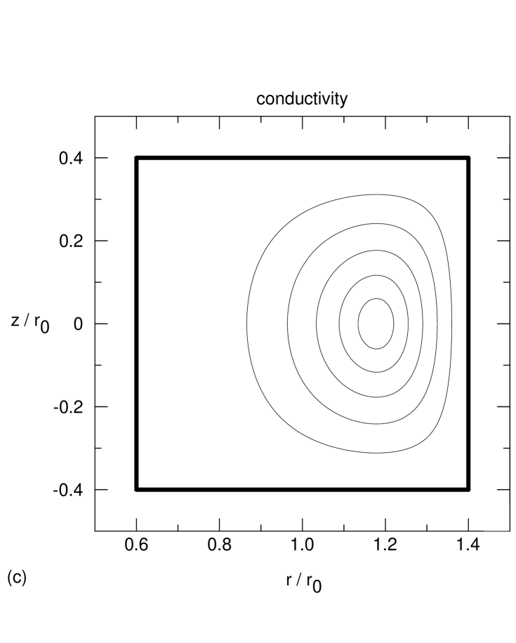
FIG. 2.: (a) Contours of constant $\psi$ (and pressure) in the case that $j_{\varphi}=\lambda r\,\psi$, for $n=0$, $\lambda\,r^{4}_{0}=29.375$, $\delta/r_{0}=0.4$, and $L/r_{0}=0.4$. (b) Current density contours, and (c) conductivity contours for the same set of parameters. The square box shows the location of the perfectly conducting, toroidal boundary. Note the non-coincidence of the conductivity contours and the magnetic surfaces. In this example, $\beta_{p}\simeq 1.2$.

- [1] G. Bateman, MHD Instabilities (MIT Press, Cambridge, 1978), pp. 59-88.
- [2] J. Wesson, Tokamaks (Clarendon Press, Oxford, 1987), pp. 60-82.
- [3] H. Grad and J. Hogan, Phys. Rev. Lett. 24, 1337 (1970).
- [4] H. Grad, Phys. Fluids 10, 137 (1967).
- [5] V. D. Shafranov, in Reviews of Plasma Physics, edited by M. A. Leontovich (Consultants Bureau, New York, 1966), Vol. 2, p. 103.
- [6] D. Montgomery and X. Shan, Comments on Plasma Phys. & Contr. Fusion 15, 315 (1994).
- [7] D. J. Acheson, Elementary Fluid Dynamics (Clarendon Press, Oxford, 1990), pp. 26-55.
- [8] J. W. Bates and H. R. Lewis, Phys. Plasmas 3, 2395 (1996).
- [9] X. Shan, D. Montgomery, and H. Chen, Phys. Rev. A 44, 6800 (1991).
- [10] X. Shan and D. Montgomery, Plasma Phys. & Contr. Fusion 35, 619 (1993); ibid 35, 1019 (1993).
- [11] X. Shan and D. Montgomery, Phys. Rev. Lett. 73, 1624 (1994).
- [12] D. Montgomery and X. Shan, in Small-Scale Structures in Three-Dimensional Hydrodynamic and Magnetohydrodynamic Turbulence, edited by M. Meneguzzi, A. Pouquet, and P. -L. Sulem (Springer-Verlag, Berlin, 1995), pp. 241-254.
- [13] J. Norbury, J. Fluid Mech. 57, 417 (1973).
- [14] For example, see G. Arfken, Mathematical Methods for Physicists, 3rd Edition (Academic Press, Inc., San Diego, 1985), p. 753.
- [15] J. P. Dahlburg, D. Montgomery, G. D. Doolen, and L. Turner, J. Plasma Phys. 40, 39 (1988).
- [16] M. L. Goodman, J. Plasma Phys. 49, 125 (1993).
- [17] D. Pfirsch and A. Schlüter, “Der Einfluß der elektrischen Leitfähigkeit auf das Gleich-gewichtsverhalten von Plasmen niedrigen Drucks in Stellaratoren,” Max-Planck-Institut Report MPI/PA/7/62 (Munich, 1962; unpublished). See also Ref. 2, pp. 88-89.