Demonstrated convergence of the equilibrium ensemble for a fast united-residue protein model

Abstract

Due to the time-scale limitations of all-atom simulation of proteins, there has been substantial interest in coarse-grained approaches. Some methods, like “Resolution Exchange,” [E. Lyman et al., Phys. Rev. Lett. 96, 028105 (2006)] can accelerate canonical all-atom sampling, but require properly distributed coarse ensembles. We therefore demonstrate that full sampling can indeed be achieved in a sufficiently simplified protein model, as verified by a recently developed convergence analysis. The model accounts for protein backbone geometry in that rigid peptide planes rotate according to atomistically defined dihedral angles, but there are only two degrees of freedom ($\phi$ and $\psi$ dihedrals) per residue. Our convergence analysis indicates that small proteins (up to 89 residues in our tests) can be simulated for more than 50 “structural decorrelation times” in less than a week on a single processor. We show that the fluctuation behavior is reasonable, as well as discussing applications, limitations, and extensions of the model.

I Introduction

How simplified must a molecular model of a protein be for it to allow full canonical sampling? This question may be important to the solution of the protein sampling problem—the generation of protein structures properly distributed according to statistical mechanics—because of the well-known inadequacy of all-atom simulations, which are limited to sub-microsecond timescales. Even small peptides have proven slow to reach convergence Lyman and Zuckerman (2006a). Sophisticated atomistic methods, moreover, which often employ elevated temperatures Swendsen and Wang (1986); Hukushima and Nemoto (1996); Hansmann (1997); Sugita and Okamoto (1999); Paschek and Garcia (2004), have yet to show they can overcome the remaining gap in timescales Zuckerman and Lyman (2006)—which is generally considered to be several orders of magnitude. On the other hand, because of the drastically reduced numbers of degrees of freedom and smoother landscapes, coarse-grained models (e.g., Refs. Levitt and Warshel, 1975; Ueda et al., 1975; Tanaka and Scheraga, 1975; Kuntz et al., 1976; Miyazawa and Jernigan, 1985; Skolnick et al., 1988; Friedrichs and Wolynes, 1989; Lau and Dill, 1989; Honeycutt and Thirumalai, 1990; Monge et al., 1995; Jernigan and Bahar, 1996; Zhou and Karplus, 1997; Liwo et al., 1997a, b; Clementi et al., 2000a; Smith and Hall, 2001; Shimada and Shakhnovich, 2002; Izvekov et al., 2004; Zuckerman, 2004) may have the potential to aid the ultimate solution to the sampling problem, particularly in light of recently developed algorithms like “Resolution Exchange” Lyman et al. (2006); Lyman and Zuckerman (2006b) and related methods Lwin and Luo (2005); Christen and van Gunsteren (2006); Liu and Voth (2007).

Although the Resolution Exchange approach, in principle, can produce properly distributed atomistic ensembles of protein configurations, it requires full sampling at the coarse-grained level Lyman et al. (2006); Lyman and Zuckerman (2006b). While the potential for such full sampling has been suggested by some studies of folding and conformational change (e.g., Refs. Clementi et al., 2000b; Zuckerman, 2004), convergence has yet to be carefully quantified in equilibrium sampling of folded proteins. How much coarse-graining really is necessary? What is the precise computational cost of different approaches? This report begins to answer these questions by studying a united-residue model with realistic backbone geometry.

We will require a quantitative method for assessing sampling. A number of approaches have been suggested Karpen et al. (1993); Straub et al. (1994); Smith et al. (2002); Elmer and Pande (2004); Lyman and Zuckerman (2006a), but we rely on a recently proposed statistical approach which directly probes the fundamental configuration-space distribution Lyman and Zuckerman (2006a); Lyman and Zuckerman . The method does not require knowledge of important configurational states or any parameter fitting. In essence, the approach attempts to answer the most fundamental statistical question, “What is the minimum time interval between snapshots so that a set of structures will behave as if each member were drawn independently from the configuration-space distribution exhibited by the full trajectory?” This interval is termed the structural decorrelation time $\tau_{\text{dec}}$, and the goal is to generate simulations of length $t_{\text{sim}}\gg\tau_{\text{dec}}$.

In this report, we demonstrate the convergence of the equilibrium ensemble for several proteins using a fast, united-residue model employing rigid peptide planes. The relative motion of the planes is determined by the atomistic geometry embodied in the $\phi$ and $\psi$ dihedral-angle rotations, as explained below. We believe such realistic backbone geometry will be necessary for success in Resolution Exchange studies. The use of geometric look-up tables enables the rapid use of only two degrees of freedom per residue ($\phi$ and $\psi$), and one interaction site at the alpha-carbon. The simulations are therefore extremely fast. Gō interactions stabilize the native state while permitting substantial fluctuations in the overall backbone.

After the model and the simulation approach are explained, the fluctuations are compared with experimental data from X-ray temperature factors and the diversity of NMR structure sets. The simulations are then analyzed for convergence and timing.

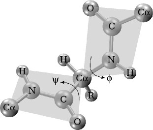
Figure 1: The rigid peptide plane model used this study. Note that, in the coarse-grained simulations, only alpha-carbons are represented, and the only degrees of freedom are $\phi$ and $\psi$. Other atoms are shown in the figure only to clarify the geometry and our assumption of rigid peptide planes.

II Coarse-grained model

The coarse-grained model used for this study was chosen to meet several criteria: (i) the fewest number of degrees of freedom per residue; (ii) the ability to utilize lookup tables for enhanced simulation speed; (iii) the stability of the native state along with the potential for substantial non-native fluctuations; and, (iv) the ability to allow the addition of chemical detail, as simply as possible. Thus, we chose a rigid peptide plane model with Gō interactions Ueda et al. (1975, 1978); Gō and Taketomi (1978) and sterics based on alpha-carbon interaction sites as shown in Fig. 1. The use of such a simple model, we emphasize, is consistent with our goal of understanding both the potential, and the limitations of coarse models for statistically valid sampling. Once we have understood the costs associated with the present model, we can design more realistic models, as discussed below. In other words, we made no attempt to design the most chemically realistic coarse-grained model, although we believe the use of atomistic peptide geometry is an improvement over a coarse model we considered previously Zuckerman (2004).

The rigid peptide planes allows the use of only two degrees of freedom per residue, arguably the fewest that one would consider in such a model. Indeed, this is fewer than in a freely rotating chain, although admittedly our model requires somewhat more complex simulation moves, described below.

Gō interactions were used because they simultaneously stabilize the native state of the protein and also permit reasonable equilibrium fluctuations, as was shown in an earlier study Zuckerman (2004). Given our interest in native-state fluctuations and the lack of a universal coarse-grained model capable of stabilizing the native state for any protein, Gō interactions are a natural choice for enforcing stability. Further, beyond the reasonable “local” fluctuations shown below, the model also exhibits partial unfolding events which are expected both theoretically and experimentally Careaga and Falke (1992); Bai et al. (1995); Eisenmesser et al. (2005).

Because we see the present model as only a first step in the development of better models, it is important that it easily allows for the addition of chemical detail, such as Ramachandran propensities which require only the dihedral angles we use explicitly Lovell et al. (2003). Furthermore, with a rigid peptide plane, the locations of all backbone atoms—and the beta carbon—are known implicitly. Thus hydrogen-bonding and hydrophobic interactions Lau and Dill (1989) can be included in the model with little effort. In other words, the “extendibility” of the present simple model was a significant factor in its design.

II.1 Potential energy of model system

The total potential used in the model is given by

$$U=U^{\rm nat}+U^{\rm non},$$ (1)

where $U^{\rm nat}$ is the total energy for native contacts, and $U^{\rm non}$ is the total energy for non-native contacts.

For the Gō interactions, all residues that are separated by a distance less than $R_{\rm cut}$ in the experimental structure are given native interaction energies defined by a square well:

$$U^{\rm nat} =\sum_{\{i<j\}}^{\rm native}u^{\rm nat}(r_{ij}),$$

$$u^{\rm nat}(r_{ij}) =\left\{\begin{array}[]{l}\infty\;\;{\rm if}\;\;r_{ij}<r_{ij}^{\rm nat}(1-\delta)\\ -\epsilon\;\;{\rm if}\;\;r_{ij}^{\rm nat}(1-\delta)\leq r_{ij}<r_{ij}^{\rm nat}(1+\delta)\\ 0\;\;{\rm otherwise}\end{array}\right.,$$ (5)

where $r_{ij}$ is the $C_{\alpha}-C_{\alpha}$ distance between residue $i$ and $j$, $r_{ij}^{\rm nat}$ is the the distance between the residues in the experimental structure, $\epsilon$ determines the energy scale of the native Gō attraction, and $\delta$ is a parameter to choose the width of the well. All residues that are separated by more than $R_{\rm cut}$ in the experimental structure are given non-native interaction energies defined by

$$U^{\rm non} =\sum_{\{i,j\}}^{\rm non-native}u^{\rm non}(r_{ij}),$$

$$u^{\rm non}(r_{ij}) =\left\{\begin{array}[]{l}\infty\;\;{\rm if}\;\;r_{ij}<(\rho_{i}+\rho_{j})(1-\delta)\\ +h\epsilon\;\;{\rm if}\;\;(\rho_{i}+\rho_{j})(1-\delta)\leq r_{ij}<R_{\rm cut}\\ 0\;\;{\rm otherwise}\end{array}\right.,$$ (9)

where $\rho_{i}$ is the hard-core radius of residue $i$ defined as half the $C_{\alpha}$ distance to the nearest non-covalently-bonded residue, and $h$ determines the strength of the repulsive interaction.

For this study, parameters were chosen to be similar to those in Ref. Zuckerman, 2004, i.e., $\epsilon=1.0$, $h=0.3$, $\delta=0.1$, and $R_{\text{cut}}=8.0$ Å.

II.2 Monte Carlo simulation

The protein fluctuations were generated using Metropolis Monte Carlo Metropolis et al. (1953). Trial configurations were generated by adding a random Gaussian deviate to the values of three sequential pairs of backbone torsions (three $\phi$ and three $\psi$ angles). We found that changing six sequential backbone torsions maximizes the rate of convergence of the equilibrium ensemble (data not shown). The energy of the trial configuration was then determined using Eq. (1), and the conformation was accepted with probability $\min(1,e^{-\Delta U/k_{B}T})$, where $\Delta U$ is the total change in potential energy of the system. The width of the Gaussian distribution for generating random deviates was chosen such that the acceptance ratio was about 40% for all simulations. The choice of temperature is discussed below.

II.3 Use of lookup tables

The speed of the coarse-grained simulation was enhanced by using lookup tables to avoid unnecessary computation. In general, utilizing lookup tables increases memory usage while decreasing the number of computations. Since memory is inexpensive and can be expanded easily, utilizing as much memory as possible can be an effective technique for increasing the speed of simulations.

In our model there are only two degrees of freedom per residue ($\phi,\psi$), but $C_{\alpha}$ distances $r_{ij}$ must be computed to determine native and non-native interaction energies given by Eqs. (5) and (9). All peptide planes are considered to possess ideal, rigid geometry as determined by energy minimization of the all-atom OPLS forcefield Jorgensen et al. (1996) using the tinker simulation package Ponder and Richard (1987).

Given a sequence of three residues (alpha carbons), we employed a lookup table to provide the Cartesian coordinates of the third residue—starting from the N-terminus—and its normal vector as a function of $\phi$ and $\psi$; see Fig. 1. The table values assume that the first residue is at the origin and the second residue is located on the z-axis. Once the coordinates for the third residue were determined via the lookup table, the fourth residue position was determined using the lookup table in conjunction with a coordinate rotation and shift. Continuing in this fashion, coordinates for the entire protein were determined.

The resolution of the lookup table is an important consideration, i.e., the number of $\phi,\psi$ values for which Cartesian coordinates are stored. In our simulations, we tried resolutions as high as $0.1^{\circ}$ and as low as $1.0^{\circ}$, and found no difference between the results. Thus, all simulation results presented here use lookup tables with a resolution of $1.0^{\circ}$.

II.4 Initial protein relaxation

One perhaps unexpected complication of utilizing a rigid peptide plane model is that great care must be taken to relax the protein before simulations can be performed. Although initial values of $\phi,\psi$ are obtained from the X-ray or NMR structure, there are slight deviations from planar/ideal geometry in a real protein. These deviations, while small, can accumulate rapidly to become very large differences in the Cartesian coordinate positions of the residues. Thus, the positions of residues near the beginning of the protein will be nearly correct, while the residues near the end of the protein will likely have large errors—compared to the experimental structure being modeled—which can create severe steric clashes or even incorrect protein topology. The severity of these “errors” necessitates the use of a relaxation procedure to generate a suitable starting structure—i.e., a set of $\phi$ and $\psi$ angles which, with our ideal-geometry peptide planes, lead to a topologically reasonable and relatively clash-free structure.

Before we detail our relaxation procedure, we note that the need for this additional calculation is an artifact of the simplicity of our model which can be overcome. With the use lookup tables, in fact, it is possible to include flexible peptide planes without significantly increasing the computational cost of the model. Such an approach, which does not require initial relaxation, is currently under investigation with promising preliminary results (data not shown).

The relaxation procedure employed in the present study first uses the $\phi,\psi$ values directly obtained from the experimental structure. These dihedrals provide the initial (problematic) structure for a coarse-grained simulation. Due to the deviations from planarity described above, the root means-square deviation (RMSD) between the initial structure we create and the experimental structure tends to be large ($\sim 10$ Å was not uncommon for the proteins in this study). To increase the number of native contacts and reduce the number of steric clashes, we next performed what we term “RMSD Monte Carlo” to relax the protein to a low RMSD structure. Trial moves for RMSD Monte Carlo were created as described above, but accepted with probability $\min(1,e^{-\Delta(\text{RMSD})/k_{B}T_{\text{RMSD}}})$, where $k_{B}T_{\text{RMSD}}=10^{-7}$ was chosen so that moves to a higher RMSD were rare. In other words, the energy function itself was not used in this initial phase.

Since residues near the beginning of the protein have less error in the starting structure than residues near the end, we used RMSD Monte Carlo in segments. The first twenty residues were relaxed until the RMSD was constant within a tolerance of 0.0001 Å, followed by the first forty, then the first sixty and so on until the RMSD of the entire protein was relaxed. The RMSD Monte Carlo simulation typically brought the RMSD of the simulated structure to less than 0.5 Å, however, there were generally still steric clashes, and some native contacts were still not present.

The final stage of relaxation was to do regular (i.e., using energy) Metropolis Monte Carlo simulation, with a very low temperature.

Relaxation was performed until four criteria were met: (i) the number of native contacts in the relaxed structure was equal to that in the NMR or X-ray structure; (ii) no steric clashes were present; (iii) no non-native contacts were present, i.e., $U^{\rm non}=0$ in Eq. (9), and; (iv) the RMSD was less than 1.0 Å. When these criteria were met the structure was saved and used as the starting configuration in all future simulations of the protein.

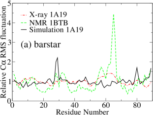
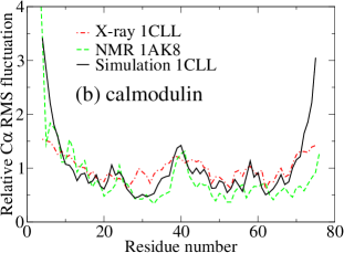
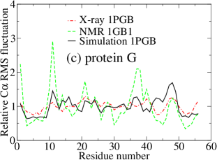
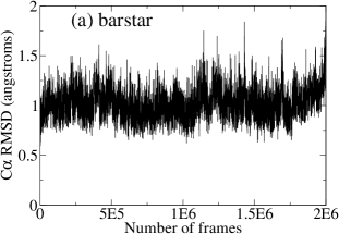
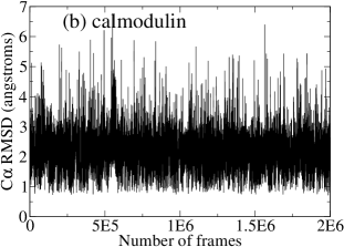
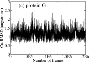
Figure 2: (Color online) Relative alpha-carbon root mean square fluctuations for three different proteins: (a) barstar, (b) calmodulin, and (c) protein G. Each plot shows results for the X-ray structure (dot-dash), the NMR ensemble (dash), and the coarse-grained simulation (solid). X-ray results were given by $\sqrt{3B/8\pi^{2}}$, where $B$ is the temperature factor given in the PDB entry. NMR and simulation data were generated using the g_rmsf program in the gromacs molecular simulation package Van Der Spoel et al. (2005); each ensemble was aligned to the first structure in the corresponding trajectory. For each coarse-grained simulation, $2\times 10^{9}$ Monte Carlo steps were performed with snapshots saved every 1000 steps, and the potential energy (1) was set up using the X-ray structure. Panels (d) - (f) show the corresponding whole-structure fluctuations as indicated by the RMSD from the experimental structures.

III Results and Discussion

Using the coarse-grained protein model described above, we generated and tested equilibrium ensembles for three proteins: barstar (PDB entry 1A19, residues 1-89), the N-terminal domain of calmodulin (PDB entry 1CLL, residues 4-75), and the binding domain of protein G (PDB entry 1PGB, residues 1-56)

For each protein, the initial simulation structure was generated, followed by RMSD and energy relaxation, as described in Sec. II.4. Then, production runs of $2\times 10^{9}$ Monte Carlo moves were performed with snapshots saved every 1000 moves, generating an equilibrium ensemble with $2\times 10^{6}$ frames.

In an attempt to obtain consistent results for the three proteins, we chose the temperature of the simulation, $k_{B}T$, to be slightly below the unfolding temperature of the protein. The unfolding temperature was determined by running simulations over a broad range of temperatures and studying the RMSD as a function of simulation time. The temperatures used in the simulations were $k_{B}T=0.6$ for barstar, $k_{B}T=0.4$ for calmodulin and $k_{B}T=0.5$ for protein G.

III.1 Speed of simulations

Due to the use of lookup tables for coordinate transformations, the small number of degrees of freedom, and utilizing simple square potentials, the equilibrium ensembles were generated very rapidly.

Running on one Xeon 2.4 GHz processor, $2\times 10^{9}$ Monte Carlo moves with snapshots saved every 1000 steps took roughly 6 days for barstar, 4 days for calmodulin, and 3 days for protein G. Thus, less than a week was required to obtain well-converged (see Sec. III.3) simulations of these coarse-grained proteins.

III.2 Protein fluctuations

We first sought to determine whether fluctuations in the coarse-grained simulation are reasonable. Figure 2 shows the alpha-carbon relative root mean square fluctuation for three different proteins. The figures show that there is reasonable qualitative agreement between the NMR, X-ray and simulation data.

It should be noted that, in fact, none of the three data sets in Figs. 2a, b and c represents the true fluctuations in the protein—for different reasons. The X-ray temperature factor, in addition to thermal fluctuations, includes crystal lattice artifacts and other experimental errors Northrup et al. (1980). NMR ensembles tend to be biased, perhaps severely, toward low energy structures, and thus also do not represent equilibrium ensembles Spronk et al. (2003). Finally, our simulation data is not accurate due to the lack of chemical detail in the forcefield.

In spite of the limitations of the analysis, we conclude from Fig. 2 that the fluctuations of the coarse-grained model are in fact reasonable.

The bottom panels of Fig. 2 show the whole-molecule fluctuations exhibited throughout the trajectories. In addition to the ability to sample large conformational fluctuations—such as in the case of calmodulin and, to a lesser degree, for protein G—the trajectories are visibly more converged than is typically observed in atomistic simulations, where RMSD values rarely reach a plateau value, let alone sampling around that plateau value multiple times as would be desirable.

III.3 Convergence analysis

The primary purpose of this report is to demonstrate the convergence of the equilibrium ensemble for a coarse-grained protein. The details of the convergence analysis are described in Ref. Lyman and Zuckerman, , so we will only briefly describe the method here.

Previously, Lyman and Zuckerman Lyman and Zuckerman (2006a) developed an approach which groups sampled conformations into structural histogram bins, using the RMSD as a metric. While promising, the primary limitation of the method was the lack of a quantitative measure of the convergence.

In the method used here, convergence was analyzed by studying the variance of the structural histogram bin populations Lyman and Zuckerman . The new approach allows a rigorous quantitative estimation of convergence—the structural decorrelation time $\tau_{\text{dec}}$, given by the time between frames required for the variance to reach an analytically computable independent-sampling value. Intuitively, and mathematically, $\tau_{\text{dec}}$ is the time interval between snapshots for which they behave as if each frame were drawn independently. If simulation times $t_{\text{sim}}\gg\tau_{\text{dec}}$ are obtained, the equilibrium ensemble is considered converged.

Perhaps the most important feature of the convergence analysis for our study is that the method does not require any prior knowledge of important states. Furthermore, there is no parameter-fitting or subjective analysis of any kind.

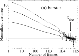
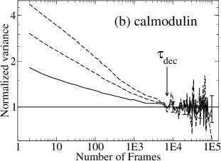
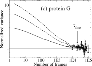
Figure 3: Convergence analysis for coarse-grained simulations of three different proteins: (a) barstar, (b) calmodulin, and (c) protein G. Each plot shows the convergence properties for the same trajectories as used for Fig. 2, analyzed using the procedure in Ref. Lyman and Zuckerman, . The number of frames required to reach the value of one (the solid horizontal line) is an approximation of the structural decorrelation time $\tau_{\text{dec}}$ and is shown on each plot. The three curves on each plot are results for different histogram sub-sample sizes Lyman and Zuckerman and demonstrates the robustness of the value of $\tau_{\text{dec}}$. The plots predict that the decorrelation times are roughly 40 000 frames for barstar, 20 000 frames for calmodulin and 30 000 frames for protein G. Note that the total number of frames generated for each protein during the simulation was $2\times 10^{6}$. Thus, since each simulation was more than $50\tau_{\text{dec}}$ in length, we conclude that the equilibrium ensembles are well-converged. Error bars represent 80% confidence intervals in the expected fluctuations around the ideal value of one, based on the given trajectory length and the numerical procedure used to generate the solid curve.

Figure 3 shows the convergence properties of the coarse-grained simulations using the same trajectories as in Fig. 2. The ratio of the observed variance to the ideal variance for independent sampling is plotted as a function of the time between the configurations used to compute the observed variance. When this ratio decreases to one the structural decorrelation time $\tau_{\text{dec}}$ has been reached, as shown in the figure. The analysis predicts that each simulation is at least 50 times longer than the structural decorrelation time.

Thus we conclude that, in less than a week of single-processor time, the equilibrium ensembles for these three proteins are well converged.

IV Conclusions

We have demonstrated the convergence of the equilibrium ensemble for a simple united-residue protein model. The model assumes rigid peptide planes, with atomistically correct geometry, and exhibits reasonable residue-level fluctuations based the planes’ geometry, Gō interactions, and sterics.

Most importantly, the results indicate quantitatively that carefully designed united-residue models have the potential to fully sample protein fluctuations. By using only two degrees of freedom per residue, look up tables for coordinate transforms, and simple square well potentials, we were able to demonstrate that converged equilibrium ensembles can be obtained in less than a week of single processor time. The quantitative convergence analysis indicates that more than 50 “decorrelation times” were simulated in each case, indicating high-precision ensembles. In addition to application in Resolution Exchange sampling of all-atom models Lyman et al. (2006); Lyman and Zuckerman (2006b), such speed opens up the long-term possibility of large-scale simulation of many proteins.

One important practical limitation of the ideal-peptide-plane geometry in the present model is the need to relax the the initial structure. Proteins larger than 100 residues are difficult to relax. However, we have already begun investigating a flexible-plane model incorporating lookup tables which exhibits no such limitation and remains computationally affordable. We will report on the flexible model in the future.

Although the intrinsic atomistic geometry of the peptide plane was included in our model, it lacks chemical interactions. Yet because we obtained converged ensembles in such a short time, it is clear we can “afford” extensions to the model which include realistic chemistry. For instance, additional potential energy terms such as Ramachandran propensities Lovell et al. (2003), hydrophobic interactions Lau and Dill (1989) and hydrogen-bonding can be included at small cost.

Aside from the potential for rigorous atomistic sampling Lyman et al. (2006); Lyman and Zuckerman (2006b); Ytreberg and Zuckerman , it is important to note the general usefulness of coarse-grained models for generating ad hoc atomistic ensembles. Specifically, upon generating a well-sampled ensemble of coarse-grained structures, atomic detail can be added using existing software such as those in Refs. Eyal et al., 2004; de Bakker et al., 2002. Once minimized and relaxed, these (now) atomically detailed structures form an ad hoc ensemble which may be of immediate use in docking Knegtel et al. (1997); Shoichet (2004) and homology modeling applications. Further, in principle, such structures can be re-weighted into the Boltzmann distribution Ytreberg and Zuckerman .

In the long term, one can imagine a day when structural databases will be based not on single (static) structures but rather will collect ensembles—as envisioned in the authors’ scheme for an “Ensemble Protein Database”(http://www.epdb.pitt.edu/).