Diffusion and dispersion of passive tracers: Navier-Stokes versus MHD turbulence

Abstract

A comparison of turbulent diffusion and pair-dispersion in homogeneous, macroscopically isotropic Navier-Stokes (NS) and nonhelical magnetohydrodynamic (MHD) turbulence based on high-resolution direct numerical simulations is presented. Significant differences between MHD and NS systems are observed in the pair-dispersion properties, in particular a strong reduction of the separation velocity in MHD turbulence as compared to the NS case. It is shown that in MHD turbulence the average pair-dispersion is slowed down for $\tau_{\mathrm{d}}\lesssim t\lesssim 10\tau_{\mathrm{d}}$, $\tau_{\mathrm{d}}$ being the Kolmogorov time, due to the alignment of the relative Lagrangian tracer velocity with the local magnetic field. Significant differences in turbulent single-particle diffusion in NS and MHD turbulence are not detected. The fluid particle trajectories in the vicinity of the smallest dissipative structures are found to be characterisically different although these comparably rare events have a negligible influence on the statistics investigated in this work.

The diffusive effect of turbulence on contaminants passively advected by the flow is of great practical and fundamental interest. While the study of passive scalars Warhaft (2000) usually reverts to the Eulerian description of the flow, the Lagrangian point of view has proven to be very fruitful regarding investigations of turbulent diffusion and pair-dispersion Yeung (2002); Sawford (2001) as well as for the fundamental understanding of turbulence Falkovich et al. (2001). The three-dimensional dynamics of passive tracers in neutral fluids has been subject of various experimental (for recent works see e.g. Voth et al. (1998); Ott and Mann (2000); Mordant et al. (2001)) and numerical, e.g. Yeung and Pope (1989); Yeung and Borgas (2004); Biferale et al. (2006); Ishihara and Kaneda (2002), investigations. Related problems regarding the turbulent diffusion of magnetic fields and the influence of turbulent magnetic fields on particle diffusion have been studied extensively in space and astrophysics, see e.g. Jokipii and Parker (1969); Giacalone and Jokipii (1999); Cattaneo (1994); Maron et al. (2004); Matthaeus et al. (1995); Pommois et al. (2001), as well as in the context of magnetically confined nuclear-fusion plasmas, see for example Rechester and Rosenbluth (1978); Krommes et al. (1983); Isichenko (1991).

This Letter reports a first effort to identify differences in the diffusion and dispersion properties of turbulent flows in electrically conducting and in neutral media. To this end the dynamics of fluid particles is studied via high-resolution direct numerical simulation of passive tracers immersed in fluids that are described by the incompressible magnetohydrodynamic (MHD) and the Navier-Stokes (NS) approximation.

Using the vorticity, $\mbox{\boldmath{$\omega$}}=\nabla\times\mbox{\boldmath{$v$}}$, and a uniform mass density, $\rho_{0}=1$, the non-dimensional incompressible MHD equations are given by

$$\partial_{t}\mbox{\boldmath{$\omega$}} = \nabla\times\left[\mbox{\boldmath{$v$}}\times\mbox{\boldmath{$\omega$}}-\mbox{\boldmath{$b$}}\times(\nabla\times\mbox{\boldmath{$b$}})\right]+\mu\Delta\mbox{\boldmath{$\omega$}}$$ (1)

$$\partial_{t}\mbox{\boldmath{$b$}} = \nabla\times\left(\mbox{\boldmath{$v$}}\times\mbox{\boldmath{$b$}}\right)+\eta\Delta\mbox{\boldmath{$b$}}$$ (2)

$$\nabla\cdot\mbox{\boldmath{$v$}} = \nabla\cdot\mbox{\boldmath{$b$}}=0\,.$$ (3)

The dimensionless molecular diffusivities of momentum and magnetic field are denoted by $\mu$ and $\eta$, respectively. The magnetic field $b$ is given in Alfvén-speed units. The Navier-Stokes equations which govern the motion of an electrically neutral fluid are obtained by setting $\mbox{\boldmath{$b$}}\equiv 0$ in Eqs. (1)-(3).

The MHD/Navier-Stokes equations are solved by a standard pseudospectral method in a triply periodic cube of linear extent $2\pi$. The velocity field at the position $X$ of a tracer particle is computed via tricubic polynomial interpolation and then used to move the particle according to

$$\dot{\mbox{\boldmath{$X$}}}(t)\equiv\mbox{\boldmath{$V$}}(t)=\mbox{\boldmath{$v$}}_{{\mathrm{intpol}}}(\mbox{\boldmath{$X$}},t)\,.$$ (4)

Eq. 4 is solved by a midpoint method which is straightforwardly integrated into the leapfrog scheme that advances the turbulent fields. Test calculations using Fourier interpolated ‘exact’ representations of turbulent velocity fields have shown that the chosen tricubic polynomial interpolation delivers sufficient precision with a mean relative error at $512^{3}$ resolution of $\sim O(10^{-3})$. In addition tricubic interpolation is numerically much cheaper than the nonlocal spline approach (cf. Yeung and Pope (1988)), especially on computing architectures with distributed memory. The initial particle positions are forming tetrads that are spatially arranged to lie on a randomly deformed cubic super-grid with a maximum perturbation of $25\%$ per super-grid cell. This configuration represents a compromise between statistical independence of particle dynamics and a space-filling particle distribution (cf. Yeung and Borgas (2004); Biferale et al. (2005)). In addition well-defined initial particle-pair separations $\Delta_{0}$ (cf. Table 1) are realized by the tetrad grouping.

Distances are given in units of the Kolmogorov dissipation length $\ell_{\mathrm{d}}=(\mu^{3}/\varepsilon^{\mathrm{K}})^{1/4}$ defined with the kinetic energy dissipation rate $\varepsilon^{\mathrm{K}}$ that is part of the total dissipation rate $\varepsilon=\varepsilon^{\mathrm{K}}+\varepsilon^{\mathrm{M}}=\int_{V}\mathrm{d}V(\mu\omega^{2}+\eta(\nabla\times\mbox{\boldmath{$b$}})^{2})$. In this work $k_{\mathrm{max}}\ell_{\mathrm{d}}\approx 1.6$. This fulfills the widely accepted resolution criterion introduced in Yeung and Pope (1989) and corresponds to a dissipative energy fall-off of about 4 decades in the dissipation range avoiding interpolation problems at grid-scales. Intervals of time are given in units of the large-eddy turnover time, $T_{0}=\pi/(2E)^{1/2}$, $E=E^{K}+E^{M}=\int_{V}\mathrm{d}V(v^{2}+b^{2})/2$ being the total energy, or in multiples of the Kolmogorov time, $\tau_{\mathrm{d}}=(\ell_{\mathrm{d}}^{2}/\varepsilon^{\mathrm{K}})^{1/3}$, as appropriate.

group	$\Delta_{0}$ (NS)	$\Delta_{0}$ (MHD)	particles	pairs
1	$1.8\ell_{\mathrm{d}}$	$2.1\ell_{\mathrm{d}}$	$4\cdot 48^{3}$	$331\,776$
2	$3.9\ell_{\mathrm{d}}$	$4.6\ell_{\mathrm{d}}$	$4\cdot 48^{3}$	$331\,776$
3	$7.9\ell_{\mathrm{d}}$	$9.2\ell_{\mathrm{d}}$	$4\cdot 36^{3}$	$139\,968$
4	$20\ell_{\mathrm{d}}$	$23\ell_{\mathrm{d}}$	$4\cdot 24^{3}$	$41\,472$
5	$98\ell_{\mathrm{d}}$	$115\ell_{\mathrm{d}}$	$4\cdot 24^{3}$	$41\,472$
total	—	—	$1\,181\,952$	$886\,464$

Table 1: Particle groups and respective initial pair separations $\Delta_{0}$

The simulations are carried out using a resolution of $512^{3}$ collocation points with aliasing errors being treated by spherical mode truncation Vincent and Meneguzzi (1991). Quasi-stationary turbulence is generated by a forcing which freezes all modes in the sphere $k\leq k_{f}=2$. The frozen modes which are taken from DNS decaying turbulence sustain the turbulence gently via nonlinear interactions. It has been checked that this way of driving does not introduce significant anisotropy by regarding direction-dependent Eulerian two-point statistics.

Starting with a set of random fluctuations of $v$ (and $b$ in the MHD case) with zero mean the driven flows reach quasi-stationary states during which the total energy $E$ shows fluctuations $\lesssim 10\%$ around unity and $E^{\mathrm{M}}/E^{\mathrm{K}}\approx 2$ (MHD). In both simulations the total energy dissipation rate $\varepsilon$ is quasi-constant at about $0.24$ with $\varepsilon^{\mathrm{M}}\approx 0.15$ in the MHD case. The turbulent fields in the MHD system have negligible magnetic and cross helicity. The macroscopic Reynolds numbers are dimensionally estimated using $\mu$, $\eta$, $\varepsilon$, $E$, and the kinetic energy $E^{\mathrm{K}}$ as $\mathsf{Re}=(E^{\mathrm{K}})^{1/2}E^{3/2}/(\varepsilon\mu)$ (hydrodynamic) and $\mathsf{Rm}=\mathsf{Re}\mathsf{Pr_{m}}$ (magnetic) with the magnetic Prandtl number $\mathsf{Pr_{m}}=\mu/\eta$ set to unity. The respective numerical values of the parameters are $\mu=8\times 10^{-4}$, $\mathsf{Re}\approx 5400$ (NS) and $\mu=\eta=5\times 10^{-4}$, $\mathsf{Re}\approx 5200$ (MHD). Cases with $\mathsf{Pr_{m}}\neq 1$ while interesting due to their importance in the context of turbulent dynamos (see e.g. Ponty et al. (2005); Schekochihin et al. (2005)) are beyond the scope of this paper and will be addressed in future work.

After the runs have reached macroscopic quasi-equilibrium the trajectories of massless point particles marking the fluid are traced over $13.5T_{0}$ (NS) and $11T_{0}$ (MHD) corresponding to $500\tau_{\mathrm{d}}$ and $350\tau_{\mathrm{d}}$, respectively. The initial particle positions are chosen in five groups of tetrads with different particle-pair separations (cf. Table 1).

In statistically isotropic turbulence single tracer particles are expected Taylor (1922) to show a diffusive time dependence of the mean-square particle displacement $\langle(\mbox{\boldmath{$X$}}(t)-\mbox{\boldmath{$X$}}_{0})^{2}\rangle\sim t$, $\mbox{\boldmath{$X$}}_{0}=\mbox{\boldmath{$X$}}(0)$, for $t\gg T_{\mathrm{L}}$ where $T_{\mathrm{L}}$ is the autocorrelation time of the Lagrangian velocity $\mbox{\boldmath{$V$}}(t)$. Here, $T_{\mathrm{L}}\approx 16\tau_{\mathrm{d}}$ (NS) and $T_{\mathrm{L}}\approx 15\tau_{\mathrm{d}}$ (MHD). If $t\ll T_{\mathrm{L}}$ ballistic scaling is predicted, $\langle(\mbox{\boldmath{$X$}}(t)-\mbox{\boldmath{$X$}}_{0})^{2}\rangle\sim t^{2}$.

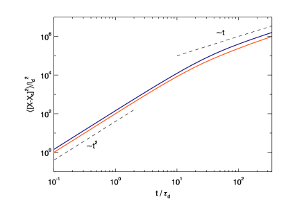
Figure 1: Evolution of normalized mean-square distance to initial position for turbulent single-particle diffusion in Navier-Stokes (black) and MHD turbulence. The dashed lines indicate ballistic scaling $\sim t^{2}$ and diffusive behavior.

In both simulations (cf. fig. 1) ballistic scaling can be identified up to about $T_{\mathrm{L}}$. Diffusive behavior is observed for $t\gtrsim 50\tau_{\mathrm{d}}$. At $t\gtrsim 70\tau_{\mathrm{d}}$ the particles have traveled about $500\ell_{\mathrm{d}}$, i.e. half the size of the simulation volume, and finite-size effects as well as the influence of the large-scale driving can be detected. The normalized turbulent diffusion coefficient $D_{\mathrm{turb}}(t_{*})=\int_{0}^{t_{*}}\mathrm{d}\tau\langle\mbox{\boldmath{$V$}}(t)\mbox{\boldmath{$V$}}(t+\tau)\rangle/\langle\mbox{\boldmath{$V$}}^{2}(t)\rangle$ with the avergage running over all trajectories shows for both systems in the interval $0<t_{*}\lesssim 50\tau_{\mathrm{d}}$ a steep increase with a subsequent saturation at the asymptotic value $T_{\mathrm{L}}$.

It is found that with regard to turbulent single-particle diffusion the NS and the MHD system show no significant differences. The small offset of the MHD displacement curve compared to the NS simulation is explained by the lower level of kinetic energy in the MHD system which is not fully compensated by the applied normalization. An analytically predicted slowing down of diffusion (and dispersion) Kim (2000) is not found here. The cited result is however based on the restricting assumption of a velocity field which is delta-correlated in time thereby neglecting the dynamically important adaptation of the velocity fluctuations to the magnetic field structure.

The observed similarity of the curves in fig. 1 indicates that statistics of single-particle trajectories is not a proper instrument to study the structural differences in the velocity field of the NS and MHD systems caused by macroscopically isotropic magnetic field fluctuations (cf. Müller and Biskamp (2000); Biskamp and Müller (2000); Haugen et al. (2004) for numerical simulations).

In this respect a more instructive diagnostic is relative pair-separation or dispersion statistics where the separation, $\mbox{\boldmath{$\Delta$}}=\mbox{\boldmath{$X$}}_{1}(t)-\mbox{\boldmath{$X$}}_{2}(t)$, of two particles is considered Batchelor (1950). The pair-separation in the ballistic regime, $t\ll\tau_{\mathrm{d}}$, where the particle velocities are finite and constant obeys the relation $\langle(\mbox{\boldmath{$\Delta$}}(t)-\mbox{\boldmath{$\Delta$}}_{0})^{2}\rangle\sim t^{2}$ (see Ott and Mann (2000) for experimental and Yeung and Borgas (2004); Biferale et al. (2006) for numerical results (all NS)) while for $t\gg T_{\mathrm{L}}$ diffusive scaling holds, $\langle(\mbox{\boldmath{$\Delta$}}(t)-\mbox{\boldmath{$\Delta$}}_{0})^{2}\rangle\sim t$ since the dynamics of particles forming a pair are statistically independent in this case.

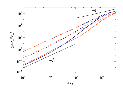
Figure 2: Evolution of normalized mean-square relative dispersion in Navier-Stokes (black) and MHD turbulence. The behavior for three different initial pair-separations (particle groups in Table 1) are shown, solid: group 1, dashed: group 3, dash-dotted: group 5. Straight lines denote ballistic $\sim t^{2}$ and diffusive scaling.

The asymptotic limits can be identified in fig. 2 with differences between NS and MHD statistics showing up at intermediate times. For clarity, only data based on the particle groups 1, 3, and 5 (cf. Table 1) are shown. In both systems the evolution of groups 2 and 4 is qualitatively similar to the behavior of group 3. As expected ballistic scaling $\sim t^{2}$ is visible in both simulations for short times up to about $\tau_{\mathrm{d}}$. Eventually, for $t\gtrsim 160\tau_{\mathrm{d}}$ an approach to the diffusive limit is seen rudimentally. The dispersion is accelerating during $10\lesssim t\lesssim 100$. However, neither the Batchelor law Batchelor (1950), $\langle(\mbox{\boldmath{$\Delta$}}-\mbox{\boldmath{$\Delta$}}_{0})^{2}\rangle=11/3C_{2}(\varepsilon\Delta_{0})^{2/3}t^{2}$, (cf. Bourgoin et al. (2006)) nor Richardson scaling Richardson (1926), $\langle\mbox{\boldmath{$\Delta$}}^{2}\rangle\sim\varepsilon t^{3}$, (cf. Ott and Mann (2000); Ishihara and Kaneda (2002)) can be clearly identified since the simulations do not generate sufficiently large inertial ranges. In addition, the theoretical preconditions necessary for Batchelor and Richardson behavior are not satisfied in the simulations presented here. In particular, Batchelor dispersion requires $\Delta_{0}$ to lie in the inertial range Batchelor (1950) for recovering of the exact prefactor. Richardson scaling is also not expected since it would entail very large $\Delta$ in the inertial range Richardson (1926). In addition Richardson behaviour would imply an appoach of the pair-separation curves to one universal scaling law independent of $\Delta_{0}$ which is not observed here.

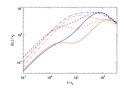
Figure 3: Normalized and averaged pair-separation velocity, $\langle U_{\parallel}\rangle$, in the direction of $\Delta$ using the same symbols as in fig. 2. Black lines: NS, grey lines: MHD

While the evolution of NS and MHD dispersion is qualitatively similar the acceleration phase in the MHD system is significantly delayed compared to the NS case. The reason for this difference is found in the averaged separation velocity $\langle U_{\parallel}\rangle$ in the direction of the separation vector $\Delta$ with $\mbox{\boldmath{$U$}}=\dot{\mbox{\boldmath{$\Delta$}}}=U_{\parallel}\mbox{\boldmath{$\Delta$}}/\Delta+\mbox{\boldmath{$U$}}_{\perp}$ shown in fig. 3 in units of $v_{\mathrm{d}}=\ell_{\mathrm{d}}/\tau_{\mathrm{d}}$. The separation velocity for all particle groups except groups 5 (cf. Table 1) which have the largest initial separation, $\Delta_{0}$, displays a continous increase before passing through a slowing-down phase for $t\gtrsim\tau_{\mathrm{d}}$. The beginning of the slowing-down marks the point of time at which the particles start to sense temporal fluctuations of the velocity field. The subsequent acceleration of dispersion can be understood by the increasing importance of sweeping by more coherent larger-scale eddies. The maximal separation velocity for all particle groups except groups 5 is reached around $90\tau_{\mathrm{d}}$ (NS) and $150\tau_{\mathrm{d}}$ (MHD). There the mean pair separation is about half the extent of the periodic simulation volume and the particles start to approach each other again. The temporal shift of the MHD maxima compared to the NS curves as seen in fig. 3 is explained by the smaller kinetic energy of the MHD system and the observed stronger slowing-down of the average MHD pair-separation velocity. The separation velocity curves for the largest initial pair-separations (groups 5) do not display the slowing-down phase since these pairs probe only the largest spatial scales of the flow where the driving is governing turbulent dynamics, cf. Yeung and Borgas (2004).

The main difference between the NS and MHD cases, however, lies in the slowing-down phase which is much more pronounced in the MHD simulation.

The reason is the well-known anisotropy of turbulent eddies with respect to the local magnetic field, see for example Shebalin et al. (1983); Goldreich and Sridhar (1995); Maron and Goldreich (2001); Cho and Vishniac (2000); Cho et al. (2002); Müller et al. (2003). Since small-scale eddies are elongated in the local magnetic field direction MHD fluid elements are more likely to travel in similar directions oriented along the local magnetic field. The field-parallel velocity component is causing the effective particle pair-separation while the field-perpendicular components are associated with Alfvénic quasi-oscillations which do not contribute to the average particle displacement. Contrary to the ballistic regime with quasi-constant flow velocities for $t\ll\tau_{\mathrm{d}}$, the anisotropy of the fluctuating velocity field at later times has a constricting effect on turbulent dispersion compared to the NS case. Consequently, the fluid particles are preferentially traveling along the magnetic lines of force which significantly reduces dispersion in the field-perpendicular directions.

Figure 4: Probability distributions of the angle $\gamma$ between the relative velocity $\mbox{\boldmath{$U$}}=\dot{\Delta}$ of particles in group 1 (cf. Table 1) and the proxy $\overline{\mbox{\boldmath{$B$}}}=[\mbox{\boldmath{$b$}}(\mbox{\boldmath{$X$}}_{1})+\mbox{\boldmath{$b$}}(\mbox{\boldmath{$X$}}_{2})]/2$ at different times $t$ ($\tau_{\mathrm{d}}$: long-dash, $4\tau_{\mathrm{d}}$: dash-dot, $8\tau_{\mathrm{d}}$: short-dash, $64\tau_{\mathrm{d}}$: solid). The thin line denotes the distribution $P(\gamma)=(\pi/360)\sin(\gamma)$ indicating isotropic dispersion.

This conjecture is supported by fig. 4 which shows probability distributions of the angle $\gamma=\measuredangle(\mbox{\boldmath{$U$}},\overline{\mbox{\boldmath{$B$}}})$ for particle group 1 and points of time in the interval $0\leq t\leq 64\tau_{\mathrm{d}}$ introducing a rough proxy of the mean magnetic field at scale $\Delta$, $\overline{\mbox{\boldmath{$B$}}}=[\mbox{\boldmath{$b$}}(\mbox{\boldmath{$X$}}_{1})+\mbox{\boldmath{$b$}}(\mbox{\boldmath{$X$}}_{2})]/2$.

For isotropic random velocities a sinusoidal distribution (thin solid line) would be expected. However, it is seen that even for comparably large times the distribution of the angle $P(\gamma)$ exhibits a clear deviation from this behavior favoring velocities aligned with the magnetic-field proxy $\overline{\mbox{\boldmath{$B$}}}$. The observed trend to sinusoidality with increasing time is due to $\langle\Delta\rangle$ approaching the largest scales of the flow which leads to weakly correlated fluctuations in $U$ and $\overline{\mbox{\boldmath{$B$}}}$. This trend is limited by the way of forcing chosen in this work.

Apart from pair-dispersion, tracer dynamics display another interesting difference between Navier-Stokes and MHD turbulence. At smallest scales in the vicinity of the most singular dissipative structures the tracer trajectories differ significantly. In the NS simulation where the smallest flow structures are vortex filaments the fluid particles describe helical motions around the filaments (cf. also Biferale et al. (2006)). In contrast, vorticity sheets typical for smallest-scales in MHD turbulence lead to characteristic kinks in the tracer path. While the resulting trajectories are strongly different and characteristic for the respective turbulent system, these events occur too seldomly to have a measurable effect on the statistics of diffusion and dispersion regarded in this paper.

In summary it was shown by comparison of direct numerical simulations of macroscopically isotropic Navier-Stokes (NS) and nonhelical magnetohydrodynamic (MHD) turbulence that the magnetic field in MHD turbulence slows down average pair-dispersion for intermediate times, $\tau_{\mathrm{d}}\lesssim t\lesssim 10\tau_{\mathrm{d}}$, compared to NS behavior. This effect is shown to be due to alignment of turbulent velocity and magnetic field fluctuations. Significant differences in turbulent single-particle diffusion could not be detected. Fluid particle trajectories in the vicinity of the strongly dissipative structures are characteristically different although these events have a negligible influence on the statistics investigated in this work.