Efficient form of the LANS-alpha turbulence model in a primitive-equation ocean model

Abstract

The Lagrangian-Averaged Navier-Stokes alpha (LANS-$\alpha$) model is a turbulence parameterization that has been shown to capture some of the most important features of high resolution ocean modeling at lower resolution. Simulations using LANS-$\alpha$ in the POP primitive-equation ocean model resemble doubled-resolution simulations of standard POP in statistics like kinetic energy, eddy kinetic energy, and potential temperature fields. The computational cost of adding LANS-$\alpha$ is only 27% for our most efficient implementation, as compared to a factor of 8—10 for a doubling of resolution.

The LANS-$\alpha$ model improves turbulence statistics with an additional nonlinear term and a smoothed advecting velocity. In this work we investigate different kinds of smoothing techniques and their effect on the LANS-$\alpha$ model’s results and efficiency. We show that we can substitute convolution filters for full Hemlholtz inversions and produce similar results at a significantly lower expense.

When constructing filters for LANS-$\alpha$ in a primitive-equation ocean model the filter weights must be chosen carefully, otherwise a pressure-velocity instability will be excited. We show analytically that certain ranges of filter weights are unstable, and confirm this with numerical experiments. Our stability criterion also guarantees that the kinetic energy is well defined, and that the filtered velocity is smoother that the original velocity.

1 Introduction

The LANS-$\alpha$ model is a turbulence model that can reproduce some of the statistics and structures that are seen in standard simulations (without LANS-$\alpha$) at higher resolution. The LANS-$\alpha$ model accomplishes this in part by using a smoothed velocity field for the advecting velocity in the momentum and tracer equations. The question addressed in this paper is, “What is the best way to smooth the velocity field in LANS-$\alpha$?” This is not simply a matter of choosing the smoothing method that produces the best result. As a turbulence model, LANS-$\alpha$ must be extremely efficient as well; if the addition of LANS-$\alpha$ were expensive, it would be more sensible to drop the turbulence model altogether and simply run at higher resolution. Thus the choices we make in designing the LANS-$\alpha$ algorithm and smoothing filters are governed by the trade-offs of higher-resolution effects versus the cost of adding LANS-$\alpha$ to the model. We win this game if we can get the effects of, say, a doubling of resolution while only increasing the computation time by a small fraction of the time required to double the resolution with the standard model.

We have designed a LANS-$\alpha$ algorithm and smoothing filter for primitive-equation ocean models that meets this criteria of a successful turbulence model. The algorithm is presented by Hecht, Holm, Petersen, and Wingate in a closely related work [1]. The focus of the present paper is the method used to smooth the advecting velocity. In the typical LANS-$\alpha$ model derivation, the smooth velocity, ${\bf u}$, is computed from the rough velocity, ${\bf v}$, with an inverse Helmholtz operator,

$${\bf u}=\left(1-\alpha^{2}\nabla^{2}\right)^{-1}{\bf v}$$ (1)

where the namesake $\alpha$ parameter is a length scale that determines the amount of smoothing [2]. The Helmholtz inversion is the basis of comparison for other smoothing methods in this work, as this is the relationship between ${\bf u}$ and ${\bf v}$ in the original LANS-$\alpha$ equations. With it we are able to run successful simulations of LANS-$\alpha$; however, it requires an iterative solver and is therefore relatively expensive. Fortunately, local averaging methods work well in LANS-$\alpha$ and are much cheaper. In these methods, the smooth velocity is computed as a weighted average of nearby neighbors, and can be written as a convolution with the filter function $g$ as

$${\bf u}=g\ast{\bf v}=\int g({\bf x}-{\bf y}){\bf v}d^{3}y.$$ (2)

The LANS-$\alpha$ equation using a filter (sometimes called the Kelvin-filtered Navier-Stokes equation) retains Kelvin’s circulation theorem [3], which is a property of fundamental importance to LANS-$\alpha$. If the filter is properly designed, other characteristics of LANS-$\alpha$ with the Helmholtz inversion are guaranteed: ${\bf u}$ is smoother that ${\bf v}$, the energy is well defined, and LANS-$\alpha$ conserves energy in the absence of dissipation. In this paper we develop design criteria for filters that satisfy these requirements.

There is a precedent of using simple filters in LANS-$\alpha$ in large eddy simulation (LES) models. Geurts and Holm [4] used a simple three-point top-hat filter as a smoothing operator in LANS-$\alpha$ and Leray LES modeling of three-dimensional isotropic turbulent mixing. They found that the LANS-$\alpha$ and Leray models are considerably more accurate than dynamic eddy-viscosity models, and at a lower computational cost. The LANS-$\alpha$ and Leray models performed particularly well at capturing the flow features characteristic of the smaller resolved scales.

This paper is organized as follows: §2 briefly reviews the LANS-$\alpha$ equations for primitive-equations and the POP-$\alpha$ algorithm. The pressure-velocity instability, which develops with the incorrect choice of filter weights, is discussed in §3. Using an eigenvalue analysis of the discretized filter in §4, we develop design criteria for the filter weights to ensure the proper smoothing and kinetic energy properties. The results section, §5, shows that POP-$\alpha$ can produce results qualitatively similar to those of higher resolution simulations of standard POP using either the Helmholtz inversion or an filter to smooth the velocity. In the final section, §6, we compare the merits of each. The family of filters presented here produce stable simulations and are 20—50% faster than Helmholtz inversions. Filters produce better temperature statistics in the baroclinic instability model problem, while the Helmholtz inversion produces higher kinetic and eddy kinetic energy.

2 The LANS-$\alpha$ model

This section gives a brief overview of the primitive-equation version of LANS-$\alpha$ that is used in the POP-$\alpha$ code. These equations were originally derived by Holm et al. [5], and are described at length, along with the POP-$\alpha$ algorithm, by Hecht et al. [1]. The model equations are

$$\displaystyle\frac{\partial{{\bf v}}}{\partial{t}}+{\bf u}\cdot\nabla{\bf v}+u_{3}\partial_{z}{\bf v}+v_{j}\nabla u_{j}+{\bf f}\times{\bf u}=-\frac{1}{\rho_{0}}\nabla\pi+{\cal F}\left({{\bf v}}\right),$$ (3)

$$\displaystyle\frac{\partial{\pi}}{\partial{z}}=-\rho g,$$ (4)

$$\displaystyle\frac{\partial{\varphi}}{\partial{t}}+{\bf u}\cdot\nabla\varphi={\cal D}\left({\varphi}\right),$$ (5)

$$\nabla\cdot{\bf u}+\partial_{z}u_{3}=0,$$ (6)

$${\bf u}=\left(1-\alpha^{2}\nabla^{2}\right)^{-1}{\bf v},$$ (7)

$$\pi=p-\frac{1}{2}|{\bf u}|^{2}-\frac{\alpha^{2}}{2}|\nabla{\bf u}|^{2}$$ (8)

where $(v_{1},v_{2},v_{3})=({\bf v},v_{3})$ and $(u_{1},u_{2},u_{3})=({\bf u},u_{3})$ are the rough and smooth velocities, $\nabla$ is the horizontal gradient, $\varphi$ is a tracer (temperature, salinity, or a passive tracer), $\rho$ is the full density, $\rho_{0}$ is the background density, $\pi$ is a modified pressure, $p$ is the physical pressure, ${\cal F}$ and ${\cal D}$ are momentum and tracer diffusion terms [6], ${\bf f}$ is the Coriolis parameter, $g$ is gravitational acceleration, and $\alpha$ is the alpha model’s smoothing length scale. These equations are hydrostatic (4), incompressible (6), and Boussinesq ($\rho_{0}$ appears in eqn 3 but not in 4).

The principle feature of the LANS-$\alpha$ model is that the momentum equation (3) is an advection-diffusion equation for a Lagrangian-averaged velocity ${\bf v}$, while the advecting velocity is an Eulerian-averaged velocity ${\bf u}$. These names arise in the derivation of the LANS-$\alpha$ model [2], where velocities are averaged along a particle track (Lagrangian) or at a particular location (Eulerian). The Helmholtz relation (7) indicates that ${\bf u}$ is smoother that ${\bf v}$. In this paper we prefer the names rough velocity for ${\bf v}$, which is computed prognostically from (3), and smooth velocity for ${\bf u}$, which is computed diagnostically from (7). The LANS-$\alpha$ model has an additional nonlinear term $\sum_{j=1}^{3}v_{j}\nabla u_{j}$ in the momentum equation (3), which does not appear in the Leray model[2], and which allows LANS-$\alpha$ to satisfy Kelvin’s circulation theorem while conserving energy and a form of potential vorticity in the absence of dissipation [2].

In this paper, we investigate how to most effectively and efficiently smooth the rough velocity ${\bf v}$ to obtain the smooth velocity ${\bf u}$. This could be with a Helmholtz inversion, as in (7), or with a convolution using various filter functions, as in (2). LANS-$\alpha$ using a filter rather than a Helmholtz inversion still satisfies Kelvin’s circulation theorem [3]. If the proper filters are chosen, one also conserves energy and a form of potential vorticity in the absence of dissipation.

The most commonly used form of the LANS-$\alpha$ equations use a three-dimensional (3D) smoothing. In the primitive equations, which assume a thin layer approximation, this reduces to a 2D smoothing, and so our filters are horizontal-only as well. 3D smoothing may be tested at a future time, but we expect that the computational cost would be too high to justify the benefit. The Helmholtz inversion is horizontally isotropic. Thus one of the design criteria for the smoothing filter is that it is horizontally isotropic as well.

The POP primitive-equation ocean-climate model [7, 8], developed and maintained at Los Alamos National Laboratory, was augmented to include the LANS-$\alpha$ formulation [1]. POP is a split implicit/explicit code; that is, it takes an implicit step for the barotropic (vertically integrated 2D) velocity field, and takes an explicit step for the baroclinic (remaining 3D) velocity field. This is done so that the timestep is not limited by the fast free-surface gravity waves in the barotropic velocity field.

In the LANS-$\alpha$ version of POP, named POP-$\alpha$, a smooth velocity field must be computed for both the baroclinic and barotropic velocity fields. In the explicit baroclinic component of the code, the smooth baroclinic velocity, ${\bf u}$, is computed by simply smoothing ${\bf v}$. The implicit barotropic component is more complicated, and in the end a reduced version of the full barotropic algorithm, as derived from the LANS-$\alpha$ equations, was used [1]. The reduced algorithm produced nearly identical results to the full algorithm, but was three to four times faster.

A few pieces of the POP-$\alpha$ barotropic algorithm are needed to understand the pressure-velocity instability presented in the following section. The 2D barotropic velocities, denoted by capital letters, are found by integrating the full velocity from the bottom to the free surface height, $\eta$:

$${\bf U}\equiv\frac{1}{H+\eta}\int_{-H}^{\eta}{\bf u}\;\;dz,$$ (9)

where $H(x,y)$ is the ocean depth when the surface is at rest. By integrating the continuity equation (6), which states that the smooth velocity is divergence-free, we obtain a prognostic equation for the free surface height,

$$\int_{-H}^{\eta}\left(\nabla\cdot{\bf u}+\partial_{z}u_{3}\right)dz=0,$$ (10)

$$\displaystyle\frac{\partial{\eta}}{\partial{t}}+\nabla\cdot\left(H+\eta\right){\bf U}=0.$$ (11)

The free surface height now replaces the pressure in the barotropic form of the momentum equation,

$$\displaystyle\displaystyle\frac{\partial{{\bf U}}}{\partial{t}}+{\bf f}\times{\bf U}=-g\nabla\eta+{\bf G},$$ (12)

where ${\bf G}$ contains the vertically integrated forcing terms. The barotropic momentum equation is the same as the shallow water equation.

3 Pressure-velocity instability

In this section, we present an analytic stability analysis of a pressure-velocity instability that constrains the filter weights in the barotropic filter. The pressure-velocity instability is a phenomenon particular to models where a smoothed velocity field is used in the equation for free surface height $\eta$ (11). Consider a velocity field in one-dimensional (1D) discretized shallow water equations, where the pressure and velocity gridpoints are offset. If the velocity field were at the Nyquist frequency (alternating between positive and negative at each grid cell), then using the standard shallow water equations, the free surface height would raise (lower) where the velocity field converges (diverges). In either case, a pressure gradient force would ensue that would work against the tendency of the surface to undergo further deformation, providing a stabilizing effect.

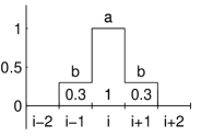
In the LANS-$\alpha$ model the equation for the free surface height involves the smooth velocity because this equation is derived from the continuity equation (6), which involves the smooth velocity. When the outer stencil weights are sufficiently large in LANS-$\alpha$, a pressure-velocity instability ensues in the highest frequencies. This can be shown with the simplest case, a 1D velocity field and a smoothing stencil of width three,

$$u_{i}=\frac{bv_{i-1}+av_{i}+bv_{i+1}}{a+2b}.$$ (13)

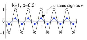
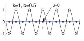
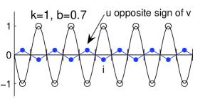
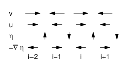
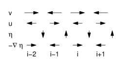
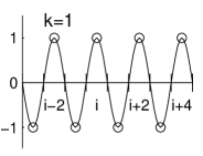
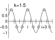
In most cases, $u_{i}$ and $v_{i}$ will have the same sign at each gridpoint, as one would expect for a smoothing operator. However, for high frequencies and sufficiently large outer stencil weight $b$, $u$ can have the opposite sign of $v$, as shown in Fig. 1 for the Nyquist frequency and $b=0.7$.

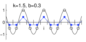
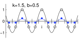
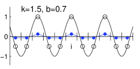
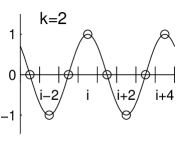
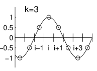
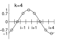
The tendency equation for $v$ depends on $\eta$, but $\eta$ in turn is not directly dependent on the convergence/divergence of $v$ but on that of $u$. In the case of a pure harmonic mode, restricting the local filter to produce a smoothed velocity $u$ of the same sign everywhere as the rough velocity $v$ is sufficient to also ensure that the divergence of smooth and rough velocities share the same sign, preserving the essential physical feedback of the underlying equations even after inclusion of the LANS-$\alpha$ model. Cases in which this physical feedback is respected or not, depending on the filter width, are illustrated in Fig. 2.

This understanding of the pressure-velocity instability allows us to construct an analytical stability criterion as follows: The filter weights must be chosen so that the filtered velocity $u$ retains the same sign as $v$ for all harmonic modes resolved on the grid.

For example, for the stencil of width three (13) where $a$ is normalized to 1, consider the Nyquist frequency

$$v_{i+j}=\cos(\pi j/k)$$ (14)

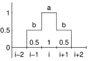
with $k=1$. Since $v_{i}=1$, the condition that $u$ and $v$ are like-signed is $u_{i}>0$. Using (13), the constraint on the stencil is $b<0.5$. For a slightly higher wavenumber, $k=1.5$, the constraint is weaker, $b<1$. For still higher wavenumbers, $u$ and $v$ are like-signed for any choice of $b$. Thus $b$ must be chosen based on the tightest constraint, $b<0.5$.

Numerical simulations of POP-$\alpha$ with a stencil of width three almost exactly correspond to the predictions of this stability analysis. The model runs stably when $b<0.48$. At larger values of $b$ an instability quickly grows in ${\bf v}$ and $\eta$ at the Nyquist frequency, so that ${\bf v}$ is four times larger than ${\bf u}$ within 100 time steps (Fig 3). By 150 timesteps the conjugate gradient routine in the barotropic solver fails to converge within 1000 iterations. Numerical simulations use a 2D stencil that is a squared version of the 1D stencil, as discussed below.

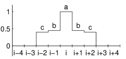
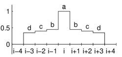
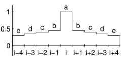
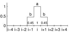
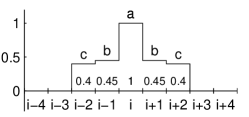
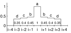
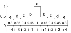
Because of the limitation imposed by the pressure-velocity instability, further smoothing must be accomplished by increasing the stencil size. The criterion that $u$ and $v$ must be like-signed for all frequencies applies, but larger stencils have more unknowns, one for each stencil weight. Figure 4 shows these constraints in chart form for 1D filters of width 3, 5, 7, and 9 and for wavenumbers $k=1\ldots 4$. In general, these constraints require that the weights are each less than $0.5$. Beyond that, each consecutive weight moving away from the center must be slightly less than the one before it. This latter requirement can be seen in the constraints for the stencil of width nine for wavenumber $k=3$ and $k=4$,

$$c+2d+e<1+b,$$ (15)

$$\sqrt{2}d+2e<1+\sqrt{2}b.$$ (16)

Neither of these are satisfied if all the weights are $0.5$, but are satisfied when the weights decrease as

$$b=0.45,\;\;c=0.4,\;\;d=0.35,\;\;e=0.3.$$ (17)

Again, the results of this stability analysis were verified using the POP-$\alpha$ model. Simulations using the stencil weights in (17) were always stable (Fig 5). If any of the weights are increased by 0.02, a fast-growing, high frequency appears in ${\bf v}$ and $\eta$ (Fig 3).

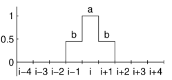
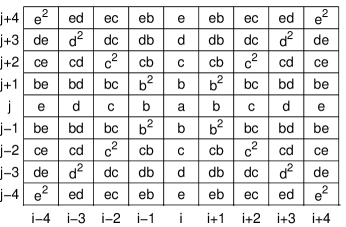
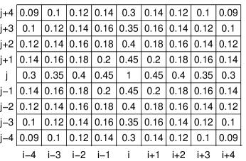
In the POP-$\alpha$ model the smoothing operator is 2D. The 2D stencil was chosen to be a squared version of the 1D stencil (Fig. 6). Such a stencil is isotropic, and thus follows the same stability analysis as the 1D case presented above. POP-$\alpha$ is very sensitive to these stability constraints; for example, if the corner weights of the stencil in Fig. 6b are increased by 10—20%, the simulation is unstable.

Other experiments were conducted where the 2D stencil was a diamond or circle instead of a square. The motivation here is that in the standard square 2D stencil (Fig. 6) the corner weights are small, and don’t contribute much to the average. Thus computation time could be saved by removing the corners from the stencil, and the degree of smoothing should be nearly the same. However, in practice any stencil other than a full square stencil resulted in unstable simulations that did not converge in the barotropic solver. This was even true when only a single gridpoint was left off of the stencil on each corner, for example when the 0.09 weight is removed from a nine-wide stencil in Fig. 6b. Thus all of the simulations presented in this work use a complete square stencil.

Near boundaries, the stencil is reduced in size so that all grid-cells used in the averaging calculation are water-cells, and none are land-cells. For example, at a grid-cell directly beside or diagonal to a land cell no averaging takes place (i.e. $u_{i,j}=v_{i,j}$). If the nearest land-cell is two grid-cells away, a filter of width three is used. The disadvantage of this method is that the smoothing goes to zero as one approaches a land-cell. This stands in contrast to the LANS-$\alpha$ equations, where the smoothing scale $\alpha$ is constant throughout the domain. Other filtering schemes near the boundary were considered: One could use a constant-size stencil and assign zero velocity to land-cells, but this strongly damps the smooth velocity near the boundary. Another possibility is to use large but nonsymmetric stencils near the boundary, but this proved to be unstable.

4 Eigenvalue analysis of the filter

Most theoretical results for the LANS-$\alpha$ model depend on the two velocities being related through the Helmholtz operator. We can replace the Helmholtz operator with filters if two critical properties are preserved. These are that (1) the filtered velocity ${\bf u}$ must be smoother than the unfiltered velocity ${\bf v}$, and (2) that the energy,

$$E=\frac{1}{2}\int{\bf u}\cdot{\bf v}\;d^{3}x$$ (18)

must be well defined (e.g., non-negative). When both of these criterion are satisfied, the filter may be used in place of the Helmholtz inversion operator in the LANS-$\alpha$ model. In this section we will review why the Helmholtz inversion satisfies these criterion, and then proceed to show that the filter described in the previous section satisfies them as well.

The Helmholtz inversion is easily shown to be a smoothing operator using Fourier analysis,

$${\hat{\bf u}}(k,l)=\frac{\hat{\bf v}(k,l)}{1+\alpha^{2}k_{h}^{2}},$$ (19)

where ${\hat{\bf u}}$ and ${\hat{\bf v}}$ are the Fourier coefficients, $(k,l)$ are horizontal wavenumbers and $k_{h}^{2}=k^{2}+l^{2}$. For scales much larger than $\alpha$ the Fourier coefficients are unaffected, because $1/k_{h}>>\alpha$ so $\alpha^{2}k_{h}^{2}<<1$ and ${\hat{\bf u}}\sim{\hat{\bf v}}$. For scales at or smaller than $\alpha$ the Fourier coefficients are strongly damped because $\alpha^{2}k_{h}^{2}>1$ so that ${\hat{\bf u}}<{\hat{\bf v}}$. The energy for the Helmholtz inversion is also well defined, because (18) can be rewritten, using integration by parts, as

$$E=\frac{1}{2}\int\left|{\bf u}\right|^{2}+\alpha^{2}\left|\nabla{\bf u}\right|^{2}\;d^{3}x,$$ (20)

which is nonnegative.

We next show that these properties also hold for our filters by using the eigenvalue problem applied to the discrete filter-operator matrix A. To illustrate this process, first consider the simple three-wide filter in 1D shown in (13). This filter can be written as a tridiagonal matrix,

$$A=\frac{1}{a+2b}\left[\begin{array}[]{cccccc}a&b&0&\cdots&0\\ b&a&b&0&\cdots\\ 0&\ddots&\ddots&\ddots&0\\ 0&\cdots&0&b&a\end{array}\right].$$ (25)

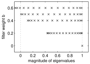
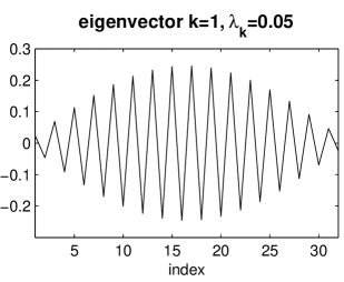
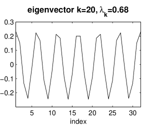
so that a vector can be filtered using ${\bf u}=A{\bf v}$. The eigenvalues of $A$ vary as a function of $b$. If $b=0$, $A$ is the identity matrix and the eigenvalues are all one. As $b$ increases, the range of eigenvalues increases but always remains less than one (Fig. 7). The smallest eigenvalues are associated with the highest wavenumber modes (Fig. 8), indicating that the most oscillatory modes are damped the strongest, and that the matrix $A$ is indeed a smoothing operator.

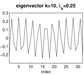
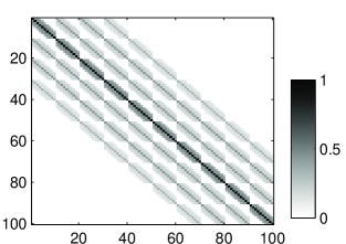
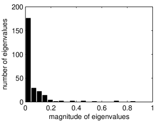
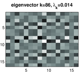
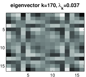
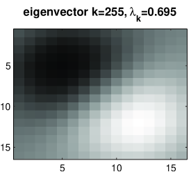
We now evaluate the eigenvalues of the full filter (Fig. 6) in 2D. On an $n\times n$ grid the filter operator is an $n^{2}$ matrix (Fig. 9). Here we consider Dirichlet boundary conditions of zero, but the results are similar for periodic boundaries. As in the 1D case, all eigenvalues are less than one. We have chosen weights so that most eigenvalues are near zero but positive (Fig. 10). The most oscillatory modes have very small eigenvalues, so that these are strongly damped (Fig. 11). This ensures that the filter is a smoothing operator.

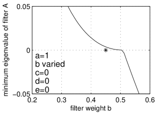
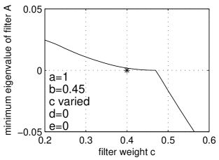
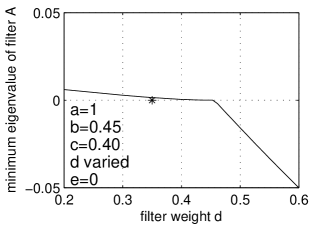
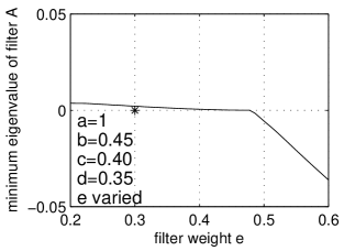
The last task is to ensure that the energy defined in (18) is well defined. The matrix $A$ is positive definite if ${\bf v}^{T}A{\bf v}>0$ for all nonzero vectors ${\bf v}$. Since the filtered velocity ${\bf u}=A{\bf v}$, this is equivalent to ${\bf v}\cdot{\bf u}>0$, which means that the global energy (18) is nonnegative and therefore well defined. A matrix is positive definite if all of its eigenvalues are positive. Thus a criterion for our filter is that its minimum eigenvalue is positive. This leads to a process for choosing each filter weight: plot the minimum eigenvalue as a function of the filter weight, and choose the largest weight that guarantees stability. There is no reason to choose a smaller value, because then the filter smooths less. Figure 12 shows that this process produces the same restrictions on filter weights as the pressure-velocity instability in the previous section. In fact, the two methods of analysis agree so well that the pressure-velocity instability appears to be a physical manifestation of the poorly defined energy. Numerical experiments where the filter weights were varied confirm that the simulations are unstable when the energy is poorly defined.

5 Results

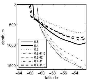
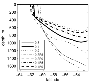
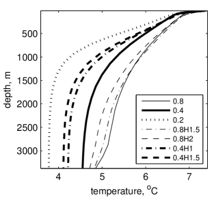
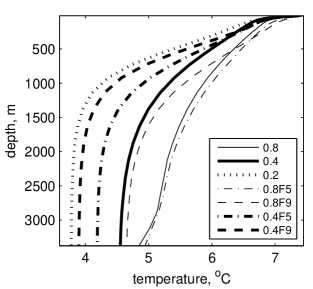
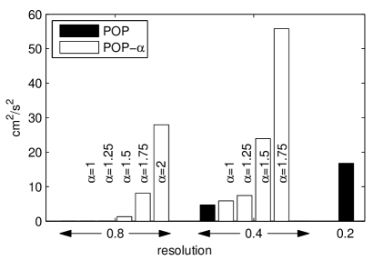
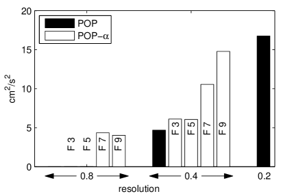
The model problem is a zonally periodic channel with a deep-sea ridge, eastward wind forcing, and surface thermal forcing that restores SST to a smooth profile from 12^oC in the north to 2^oC in the south, as described in [1]. This configuration is an idealization of the Antarctic Circulpolar Current, and was designed to induce baroclinic instability, where isopycnals are tilted from the horizontal meridionally by the surface thermal and wind forcing. If present, eddies in the flow advect heat meridionally, with the net effect that the isopycnals are less tilted; in this way, the eddies convert the potential energy of the tilted isopycnals to the kinetic energy of the eddies themselves. Simulations of standard POP at three resolutions show this effect. In the lowest resolution simulation (0.8, see Table 1) the Rossby Radius of deformation is not resolved, and no eddies are present. As the resolution doubles (0.4) and doubles again (0.2) more eddies exist, and the isopycnals are less tilted (Fig. 13).

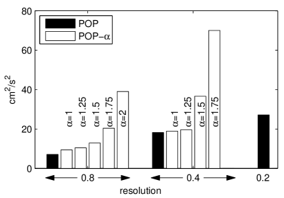
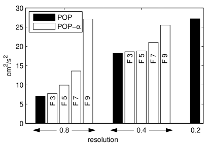
The flatter isotherms at higher resolution create a sharper thermocline and colder temperatures below the thermocline (Fig. 14). (In this model configuration, salinity is constant, so the isotherms shown in the figures coincide with isopycnals.) Higher resolution simulations of standard POP also show progressively higher kinetic energy (Fig. 15) and higher eddy kinetic energy (Fig. 16) as more eddies are resolved.

POP-$\alpha$ simulations resemble higher resolution simulations of standard POP in all of these measures. The strength of the eddy activity is controlled by how much smoothing is done on the rough velocity ${\bf v}$: when a Helmholtz inversion is used, a larger $\alpha$ smooths more; when a filter is used, wider filter stencils smooth more. In either case, Figs. 13–16 show that POP-$\alpha$ can produce results that look progressively like a doubling of resolution of standard POP as the smoothing is increased.

Because POP-$\alpha$ has two velocities, some details are necessary to explain how these diagnostic quantities were computed. The kinetic energy is

$$KE=\left(u_{1}^{2}+u_{2}^{2}\right)/2,\;\;\;KE_{\alpha}=\left(u_{1}v_{1}+u_{2}v_{2}\right)/2$$ (26)

for POP and POP-$\alpha$, where the subscripts indicate horizontal components. The eddy kinetic energy is

$$EKE=\left(\overline{(u_{1}^{\prime})^{2}}+\overline{(u_{2}^{\prime})^{2}}\right)/2,\;\;\;EKE_{\alpha}=\left(\overline{u_{1}^{\prime}v_{1}^{\prime}}+\overline{u_{2}^{\prime}v_{2}^{\prime}}\right)/2,$$ (27)

where each variable is the sum of a mean and perturbation, e.g. $u_{1}=\overline{u_{1}}+u_{1}^{\prime}$, and the overbar indicates a five-year time-averaged mean.

There would seem to be three possible ways one could compute the kinetic energy for POP-$\alpha$: using the products $u^{2}$, $uv$, or $v^{2}$. The product of the smooth and rough velocities, $uv$, is used because this the conserved kinetic energy that emerges from the derivation of the LANS-$\alpha$ equation [5, 2]. For comparison, kinetic and eddy kinetic energies were also computed using $u^{2}$ and $v^{2}$. The product of the smooth velocities is smaller than $uv$, and the product of the rough velocities is larger (typically by 10 to 20%). However, the general trends shown in Figs. 15 and 16 still hold if $u^{2}$ or $v^{2}$ are used instead of $uv$.

An interesting difference between the filter and Helmholtz inversion in POP-$\alpha$ is that simulations using filters are better at the temperature statistics, while simulations using the Helmholtz inversion have higher kinetic and eddy kinetic energy. This can be seen by comparing 0.8H2 with 0.8F9 or 0.4H1.5 with 0.4F9 if figures 13—16. Even though results differ a bit with each measure, one may loosely assign each filter an effective alpha value. For example, in most plots the filter F5 corresponds to $\alpha=1.5\Delta x$ and F9 corresponds to $\alpha=2\Delta x$.

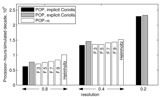
The computation time required for POP-$\alpha$ is slightly longer than standard POP due to the smoothing operations and additional nonlinear term, but is much less than a doubling of resolution in standard POP (Fig. 17). Computation increases as the filter width increases from three to nine; smoothing using the Helmholtz inversion is even slower than the nine-wide filter.

The standard POP algorithm may use an explicit or implicit discretization for the Coriolis term. Typically the implicit discretization is chosen because it allows longer timesteps to be taken, resulting in faster simulations. As described in [1], the POP-$\alpha$ algorithm must use the explicit implementation of the Coriolis term. Fortunately, POP-$\alpha$ can use longer timesteps than the standard POP algorithm with explicit Coriolis [1, 9]. This explains why most of the POP-$\alpha$ simulations in Fig. 17 are faster than POP with an explicit Coriolis term, and just a bit slower than POP with an implicit Coriolis term.

6 Conclusions

This paper presents an assessment of two methods of smoothing the velocity field in the LANS-$\alpha$ turbulence model: the Helmholtz inversion and filters. The LANS-$\alpha$ model equations specify the Helmholtz inversion, but this method requires an iterative conjugate gradient routine for each smoothing. The filter, which is simply a weighted average of nearby neighbors, results in simulations that are 20 to 50% faster than those with the Helmholtz inversion. This disparity is expected to increase with larger domains and more processors, because more iterations are required for convergence in the conjugate gradient method as the problem-size increases ([10], p. 530). The savings in computation time provides a strong motivation to choose a local filter over the global Helmholtz inversion.

Both the Helmholtz inversion and the filters produce results expected of the LANS-$\alpha$ turbulence model: statistics such as temperature profiles, kinetic and eddy kinetic energy resemble higher-resolution simulations of non-alpha simulations. The parameter $\alpha$ is a length-scale that controls the amount of smoothing, and thus the strength of the turbulence model. Analogously, as the filter width varies from three to nine, the smoothing increases and the effects of LANS-$\alpha$ are stronger. For a particular value of $\alpha$ or filter width, the methods perform a bit differently in different metrics: the filter has better temperature profiles (as judged by higher-resolution simulations), while the Helmholtz inversion has higher kinetic and eddy kinetic energy.

The filter is more robust than the Helmholtz inversion. When $\alpha$ was too high (i.e the smoothing too strong) in the Helmholtz inversion method, the kinetic energy grew without bound and the simulation was unstable. This is typical of LANS-$\alpha$ models. Unstable simulations occurred when $\alpha=2.5\Delta x$ and $2\Delta x$ at resolutions of 0.8 and 0.4, respectively. For the filter, all stencils tested (up to 9x9) were stable, and stronger sub-grid model effects could be obtained with the filter than with the Helmholtz inversion.

The stencil weights must be chosen carefully, otherwise POP-$\alpha$ will be unstable. If the outer weights are too large, the smooth velocity will be of the opposite sign as the rough velocity for the highest wave-number modes. When this occurs the pressure gradient, which is calculated from the smooth velocity, is of the wrong sign. The physically correct relationship between pressure gradient force and rough velocity is lost, and the mode grows. The conditions that bring about this pressure-velocity instability were identified exactly, and then verified by numerical simulations. We found that the first neighboring weight must be less than one-half the central weight, and each consecutive neighbor must be less than the one before. In 2D, this pattern is squared to make an isotropic, stable stencil. The full square was required; leaving off the corners to make diamond-shaped stencils resulted in unstable simulations.

It is important that the filters chosen are actually smoothing operators, and that the energy is well defined. Both of these properties were verified using an eigenvalue analysis of the filter, discretized as a matrix operator. In fact, the criterion on filter weights that guaranteed well-defined energy turned out to be the same as the weight limits to prevent the pressure-velocity instability. Thus it appears that the instability is a physical manifestation of poorly-defined energy in the equation set.

The goal of any turbulence model is to capture the effects of higher resolution simulations without paying the computational price of running at that higher resolution. We have shown that our implementation of the LANS-$\alpha$ model in a primitive-equation ocean-climate model accomplishes this goal. Specifically, statistics in POP-$\alpha$ simulations such as kinetic energy, eddy kinetic energy, and temperature profiles are similar to standard POP simulations with double the resolution. But the LANS-$\alpha$ simulations only required 27% more computing time than standard POP, as compared to a factor of nine increase to double the resolution of standard POP (for the 0.4 case).

We are currently performing simulations to compare LANS-$\alpha$ with other turbulence models, including constant coefficient hyperviscosity, Gent-McWilliams isopycnal tracer mixing [11], the Leray model [2], and the Simplified Bardina model [12]. These results, to be published in the near future, will consider the merits of LANS-$\alpha$ relative to competing models in the context of primitive-equation ocean models. We also intend to test the model in an ocean-basin or global simulation.

The comparison of the Helmholtz inversion and the filter in this study has shown that the filter is both cheaper and more robust than the Helmholtz inversion, while producing similar results. Thus our future work with the POP-$\alpha$ model will use local filters in place of the global Helmholtz for the majority of our simulations.

7 Acknowledgements

I thank M. Hecht and B. Wingate for numerous discussions, ideas, and feedback on the manuscript; E. Titi for valuable insight on the important properties of filters; and B. Geurts for helpful conversations on his experience with filters in LES models. This work was carried out under the auspices of the National Nuclear Security Administration of the U.S. Department of Energy at Los Alamos National Laboratory under Contract No. DE-AC52-06NA25396.

Figure 1: The effects of filtering the rough velocity $v$ (open circles) to compute the smooth velocity $u$ (closed circles) for a 1D filter of width three, where the weight of the neighboring cell, $b$, is varied between 0.3 and 0.7, as shown in the left column. For the Nyquist frequency ($k=1$, middle column) $u$ is of opposite sign to $v$ if $b>0.5$; this results in an instability, since the equation for free surface height $\eta$ involves $u$. For a slightly higher wavenumber ($k=1.5$, right column) $u$ has the same sign as $v$ for $b<1$.

(a) stable case, $b<0.5$	(b) unstable case, $b>0.5$

Figure 2: Schematic of variables to illustrate the pressure-velocity feedback instability. In the stable case (a) the smooth and rough velocities, $u$ and $v$, are of the same sign, and the pressure gradient force $-\nabla\eta$ counters the original velocity perturbation, as expected. In the unstable case (b), $u$ and $v$ have opposite signs; the free surface height, which is computed from $u$, increases (decreases) where $u$ converges (diverges); now the pressure gradient force reinforces the rough velocity $v$, increasing this perturbation.

(a) rough velocity $v$	(b) smooth velcotiy $u$

Figure 3: An example of the pressure-velocity instability. Shown are the velocity fields of simulation 0.8F3 using $b=0.52$ after 100 time steps. The Nyquist frequency grows exponentially in the rough velocity $v$ (a), but is filtered out of the smooth velocity $u$ (b) (note difference in vector length scales). The surface elevation $\eta$ is computed using $u$, so pressure gradient forces don’t counteract this unstable mode.

condition:	$1+2b(-1)$	$1+2b\left(-\frac{1}{2}\right)$	$1+2b(0)+2c(-1)$	$1+2b\left(\frac{1}{2}\right)$	$1+2b\left(\frac{\sqrt{2}}{2}\right)$
	$+2c(1)+2d(-1)$	$+2c\left(-\frac{1}{2}\right)+2d(1)$	$+2c(-1)+2d(0)$	$+2c\left(-\frac{1}{2}\right)+2d(-1)$	$+2c(0)+2d\left(-\frac{\sqrt{2}}{2}\right)$
	$\;\;+2e(1)>0$	$\;\;+2e\left(-\frac{1}{2}\right)>0$	$\;\;+2e(-1)>0$	$\;\;+2e\left(-\frac{1}{2}\right)>0$	$\;\;+2e(-1)>0$
	$b<\frac{1}{2}$	$b<1$	stable $\forall\>\>b$	stable $\forall\>\>b$	stable $\forall\>\>b$
	$b<\frac{1}{2}+c$	$b+c<1$	$c<\frac{1}{2}$	$c<1+b$	stable $\forall\>\>b,c$
	$b+d<\frac{1}{2}+c$	$b+c<1+2d$	$c<\frac{1}{2}$	$c+2d<1+b$	$d<\frac{\sqrt{2}}{2}+b$
	$b+d<\frac{1}{2}+c+e$	$b+c+e<1+2d$	$c<\frac{1}{2}+e$	$c+2d+e<1+b$	$\sqrt{2}d+2e<1+\sqrt{2}b$

Figure 4: Conditions required for stability for filters of width 3, 5, 7, and 9 (rows) for several wavenumbers of $v$ (columns). Variables $a$—$e$ are the weights of the 1D stencil, normalized such that $a=1$. A stable scheme requires that $u_{i}$, the smooth velocity, is the same sign as $v_{i}$. Conditions that limit the weights $b$—$e$ to be less that one-half are boxed.

(a) 1D stencil, width 3	(b) width 5
(c) width 7	(d) width 9

Figure 5: Filters used in this study, with the value of each weight $b$—$e$ under the corresponding variable.

(a) (b)

Figure 6: The 2D version of a filter stencil of width nine general form (a). This is simply the square of the 1D stencil. The 2D filters of width 3, 5, and 7 are subsets of this stencil. Our specific choice of weights is shown in (b).

Figure 7: Eigenvalues of the 1D, width-three filter operator using 16 gridpoints. When $b=0$ the operator is simply the identity, so all eigenvalues are one. As $b$ increases the eigenvalues spread out below one, indicating that some eigenvectors contract. Eigenvalues are never larger than one, so no eigenvectors increase. When $b>0.5$ there are negative eigenvalues.

(a) (b)

(c) (d)

Figure 8: Eigenvectors of the 1D, width-three filter operator using 32 gridpoints. High wavenumber modes (a,b) have eigenvalues near zero, while low wavenumber modes (c,d) have eigenvalues near one. This shows that the filter is a smoothing operator, because the highest wavenumbers are strongly damped.

Figure 9: Matrix representation of the 2D, 7x7 filter using 10x10 gridpoints. The full matrix is 100 elements square, while each block is 10 square. This matrix is not yet normalized by the factor $1/(a+2b+2c+2d+2e)^{2}$, so weights range between 0 and 1.

Figure 10: Distribution of eigenvalues of the 2D, 9x9 filter operator using 16x16 gridpoints. Filter weights are as shown in Fig. 5. The majority of eigenvalues are less than 0.1, indicating that most eigenmodes are stongly damped.

(a) (b)

(c) (d)

Figure 11: Eigenmodes of the 2D, 9x9 filter operator using 16x16 gridpoints. As in the 1D case, highly oscillatory modes (a) have eigenvalues near zero and so are strongly damped, while less oscillatory modes (d) have eigenvalues near one and so are only weakly damped. This shows that the filter we have implemented is a smoothing operator.

(a) (b)

(c) (d)

Figure 12: Minimum eigenvalue of the 2D, 9x9 filter operator using 16x16 gridpoints, as a function of each filter weight. If all eigenvalues are strictly positive then the operator is positive definite, and the energy is well defined. The value of each filter weight is chosen (starred points) to satisfy this criterion.

(a)

(b)

Figure 13: Depth of 6^oC isotherm of potential temperature using the Helmholtz inversion (a) and the filter (b) to smooth the velocity. Higher resolution simulations of standard POP (dotted line) have isotherms which are less tilted than lower resolution simulations (solid lines). As $\alpha$ or filter size increases, the POP-$\alpha$ simulations show flatter isotherms, and approach a doubling of resolution using standard POP.

(a) Helmholtz inversion	(b) filters

Figure 14: Horizontally averaged potential temperature versus depth using the Helmholtz inversion (a) and the filter (b) to smooth the velocity. Higher resolution simulations of standard POP (dotted line) are cooler and have a sharper thermocline than lower resolution simulations (solid lines). Again, POP-$\alpha$ simulations approach a doubling of resolution using standard POP.

(a) Helmholtz inversion	(b) filters

Figure 15: Kinetic energy for all simulations. As the resolution increases with standard POP, the kinetic energy increases. Kinetic energy also increases using POP-$\alpha$ at fixed resolution, when $\alpha$ is increased using the Helmholtz inversion (a) or the stencil width of the filter is increased (b). Each value was calculated by averaging over the entire domain, and in time after 500 years.

(a) Helmholtz inversion	(b) filters

Figure 16: Same as Fig. 15 but for eddy kinetic energy. Note that at the lowest resolution (0.8) the eddy kinetic energy of standard POP is indistinguishable from zero on this scale.

Figure 17: Timing data from various implementations of POP and POP-$\alpha$ (note log scale). The POP-$\alpha$ filter algorithms (F3—F9) are much cheaper than a doubling of resulution using standard POP. Using a Helmholtz inversion to smooth is more expensive than the filters. All POP-$\alpha$ algorithms use explicit Coriolis discretization.

name	model	smoothing	$\alpha$	fw	grid	lon	lat
$0.8$	POP	-	-	-	40x40x34	0.8	0.4
$0.4$	POP	-	-	-	80x80x34	0.4	0.2
$0.2$	POP	-	-	-	160x160x34	0.2	0.1
$0.8$H1	POP-$\alpha$	Helmholtz	1 $\Delta x$	-	40x40x34	0.8	0.4
$0.8$H1.5	POP-$\alpha$	Helmholtz	1.5 $\Delta x$	-	40x40x34	0.8	0.4
$0.8$H2	POP-$\alpha$	Helmholtz	2 $\Delta x$	-	40x40x34	0.8	0.4
$0.4$H1	POP-$\alpha$	Helmholtz	1 $\Delta x$	-	80x80x34	0.4	0.2
$0.4$H1.5	POP-$\alpha$	Helmholtz	1.5 $\Delta x$	-	80x80x34	0.4	0.2
$0.4$H2	POP-$\alpha$	Helmholtz	2 $\Delta x$	-	80x80x34	0.4	0.2
$0.8$F3	POP-$\alpha$	filter	-	3	40x40x34	0.8	0.4
$0.8$F5	POP-$\alpha$	filter	-	5	40x40x34	0.8	0.4
$0.8$F7	POP-$\alpha$	filter	-	7	40x40x34	0.8	0.4
$0.8$F9	POP-$\alpha$	filter	-	9	40x40x34	0.8	0.4
$0.4$F3	POP-$\alpha$	filter	-	3	80x80x34	0.4	0.2
$0.4$F5	POP-$\alpha$	filter	-	5	80x80x34	0.4	0.2
$0.4$F7	POP-$\alpha$	filter	-	7	80x80x34	0.4	0.2
$0.4$F9	POP-$\alpha$	filter	-	9	80x80x34	0.4	0.2

Table 1: Model parameters for experiments discussed in this paper, fw is the filter width; grid is the number of gridpoints in $(x,y,z)$; lon is the longitudinal grid-cell width; and lat is the latitudinal grid-cell width. The names are a concatenation of the meridional resolution, the type of smoothing, and the value of $\alpha$ or filter width.

algorithm	Cor	steps/day			clock time
		resolution			resolution
		0.8	0.4	0.2	0.	8	0.4	0.2
POP	imp	12	22	40	4.	16	21.3	195
POP	exp	20	32	52	5.	82	28.4	212
POP-$\alpha$ F3	exp	18	24		5.	09	22.7
POP-$\alpha$ F5	exp	18	24		5.	68	22.7
POP-$\alpha$ F7	exp	18	24		6.	18	25.6
POP-$\alpha$ F9	exp	18	24		6.	89	27.1
POP-$\alpha$ Helm.	exp	12	18		10.	21	33.0

Table 2: Minimimum steps/day and the resulting clock time for various algorithms and resolutions. The second column states whether the barotropic Coriolis term is implicit or exlpicit. Clock time is in processor-hours per simulated decade. The fastest POP-$\alpha$ algorithm is the reduced algorithm with a filter. Even though the POP-$\alpha$ algorithms use explicit Coriolis discretization, the timestep is larger (fewer steps per day) than standard POP with explicit Coriolis.

References

- [1] M. W. Hecht, D. D. Holm, M. R. Petersen, B. A. Wingate, Implementation of the LANS-alpha turbulence model in a primitive equation ocean model, submitted to JCP (2007).
- [2] D. D. Holm, Fluctuation effects on 3D Lagrangian mean and Eulerian mean fluid motion, Physica D133 (1999) 215–269.
- [3] C. Foias, D. D. Holm, E. S. Titi, The Navier-Stokes-alpha model of fluid turbulence, Physica D Nonlinear Phenomena 152 (2001) 505–519.
- [4] B. J. Geurts, D. D. Holm, Leray and LANS- modeling of turbulent mixing, Journal of TurbulenceSubmitted.
- [5] D. Holm, J. Marsden, T. Ratiu, The Euler-Poincare equations in geophysical fluid dynamics, Isaac Newton institute proceedings — (1998) —.
- [6] R. Smith, P. Gent, Reference manual for the Parallel Ocean Program (POP), see http://climate.lanl.gov/source/projects/climate/Models/POP (2002).
- [7] R. D. Smith, J. K. Dukowicz, R. C. Malone, Parallel ocean general circulation modeling, Physica D 60 (1992) 38–61.
- [8] J. K. Dukowicz, R. D. Smith, Implicit free-surface method for the Bryan-Cox-Semtner ocean model, J. Geophys. Res.99 (1994) 7991–8014.
- [9] B. A. Wingate, The maximum allowable time step for the shallow water alpha model and its relation to time-implicit differencing, Mon. Weather Rev.132 (12) (2004) 2719–2731.
- [10] G. H. Golub, C. F. V. Loan, Matrix Computations, 3rd Edition, Johns Hopkins Univ. Pr., 1996.
- [11] P. R. Gent, J. C. McWilliams, Isopycnal mixing in ocean circulation models, J. Phys. Oceanogr.20 (1) (1990) 150–155.
-
[12]
Y. Cao, E. M. Lunasin, E. S. Titi, Global well-posedness of the
three-dimensional viscous and inviscid simplified bardina turbulence models,
unpublished (2006).
URL http://www.citebase.org/abstract?id=oai:arXiv.org:physics/0608096