Unitary Fermi Gas in a Harmonic Trap
Abstract
We present an ab initio calculation of small numbers of trapped, strongly interacting fermions using the Green’s Function Monte Carlo method (GFMC). The ground state energy, density profile and pairing gap are calculated for particle numbers using the parameter-free “unitary” interaction. Trial wave functions are taken of the form of correlated pairs in a harmonic oscillator basis. We find that the lowest energies are obtained with a minimum explicit pair correlation beyond that needed to exploit the degeneracy of oscillator states. We find that energies can be well fitted by the expression where is the Thomas-Fermi energy of a noninteracting gas in the trap and is a pairing gap. There is no evidence of a shell correction energy in the systematics, but the density distributions show pronounced shell effects. We find the value for the pairing gap. This is smaller than the value found for the uniform gas at a density corresponding to the central density of the trapped gas.
pacs:
03.75.Ss, 05.30.Fk, 21.65.+fThe physics of cold trapped atoms in quantum condensates has seen remarkable advances on the experimental front, particularly with the possibility to study pairing condensates in fermionic systemsohara02 ; barten04 ; bourdel04 ; chin04 ; zwier05 ; kinast05 ; stewart06 . Many features of systems in the size range are now well-explored, but the small- limit is also of great interest for optical lattices. In this work we investigate the properties of small systems of trapped fermionic atoms using the Green’s Function Monte Carlo technique (GFMC) that has been successful in the study of the homogeneous gasca03 . The small systems are in some ways more challenging because simplifications that follow from translational invariance are not present. Our main goal here is to see how the bulk behavior evolves as a function of the number of atoms and to provide benchmark ab initio results to test other theoretical methods. The Hamiltonian for interacting atoms in a spherical harmonic trap is given by
| (1) |
where is the trap frequency and is the interaction between the atoms of opposite spin states. We will use units with . The interaction is chosen to approach the so-called unitary limit, meaning that it supports a two-body bound state at zero energy as well as having a range much shorter than any other length scales in the Hamiltonian. For technical reasons, we keep interaction range finite in the GFMC using the form
| (2) |
The effective range of the potential is ; the short-range limit is . The results are presented in the following sections, together with some comparison to the expectations based on the local density approximation (LDA).
To apply the GFMC, one starts with a trial wave function that is antisymmetrized according to the fermion statistics of the particles. The GFMC gives the lowest energy state in the space of wave functions that have the same nodal structure as . We tried several approaches to parameterize . For even particle number , they can all be expressed in the form
| (3) |
Here is a pair wave function, , and is a Jastrow correlation factor. The antisymetrization operation is carried out by evaluating determinant of an -dimensional matrix. For systems with an odd number of particles, we need to include an unpaired particle in the wave function. We define an orbital wave function for the extra particle and it is included by adding an extra row and column to the determinant (ca03, , Eq. 14) in the antisymmetrization. We have mostly investigated trial wave functions where the pair state takes the form he02a ; he02b ,
| (4) | |||||
Here is the oscillator state labeled by radial quantum number and angular momentum quantum numbers , the oscillator shell is , and is a shell cutoff. Clebsch-Gordan coefficients allows that the the pairs with angular momenta and to form zero total angular momentum state. The Ansatz Eq.(4) is analogous to the pair wave function used to calculation the uniform system ca03 . There the particle orbitals were plane waves and each was paired with the orbital of opposite momentum. This pair state allows for intra-shell () as well as multi-shell () pairings. At shell closures such as the trial function is equivalent to the Slater determinant of harmonic oscillator orbitals when the cutoff is at the highest occupied shell and multi-shell pairings are neglected. We have also considered taking the pair wave function as the eigenstate of the two-particle Hamiltonian, requiring in principle an infinite cutoff in the oscillator representation. We call this case as 2B.
We carry out the GFMC in the usual way described in Ref. kalos74 . The ground state wave function is projected out of the trial wave function by evolving it in imaginary time, and the energy is taken by the normalized matrix element of the Hamiltonian operator. This may be expressed as
| (5) |
and . The integral is evaluated by the Monte Carlo method, carrying out the exponentiation by the expansion and using path sampling. Our target accuracy is 1% on the energies. This is achieved by taking numerical parameters and . In practice, the convergence to the ground state is reached in the first few thousands of steps. The Monte Carlo sample points that leave the region where are discarded. This nodal constraint avoids the signal decay known as ‘fermion sign problem’. The energies depend on the range parameter only in the combination which we set to 0.1. We believe this is small enough to give energies that approach the contact limit to within 1%. Smaller values of range parameter are possible but increase the statistical fluctuations of the Monte Carlo integration.
The cases are special in that analytic solutions are known. For the system, the Jastrow correlation factor can be defined to give the exact wave function and energy . The system gives the first real test of the theory. The exact energy is , given by the solution of a transcendental equation in one variablewe06 . Using Eq. 4 with a single term () we find an energy of in close agreement with the exact value. In contrast, taking the pair wave function as the two-particle eigenstate gave a significant difference, .
We now turn to the larger systems and determine the parameters in Eq. 4. As mentioned earlier, at the shell closures taking the cutoff at the highest occupied shell gives the harmonic oscillator Slater determinant (HOSD). We also tried Slater determinants for mid-shell systems, but typically they break rotational symmetry and give a significantly higher energy. Use of Eq. 4 guarantees that will be rotational invariant (for even ). One parameterization we explored was to use the results of Ref. ca03 to guide the choice of and the . This gives a rather open trial wave function, having significant particle excitation out of the lower shells. Another choice is to take each proportional to the shell occupancy of the HOSD, which we call I1. For mid-shell systems, this also produces significant excitations out of the nominally closed shells. Both these schemes gave poorer energies than we could achieve by taking amplitudes that maximize the occupancy of the filled shells of the HOSD, and have no occupancy in the nominally empty shells. Values of that approach this compact limit (CL) are given in Table 1. As seen in this table, parameters are not very sensitive in the ranges limited by the shell closures and are kept constant.
For odd , we take the pair wave function the same as in the neighboring even system, and the orbital of the odd particle as an oscillator state of the filling shell. Thus, in the range the orbital is a -shell orbital with . Starting at there is a choice of orbitals, eg. or for . We found for the and systems, the energies are degenerate within the statistical errors and it was not possible to determine the density preference of the excitation. For these cases, we simply took the odd orbital to be one with the highest value of .
The calculated energies are summarized in Table 2 for the paired wave function in the compact limit. The statistical errors of the GFMC are given in parenthesis. One sees that an accuracy of 1% is achieved with the numerical procedure we described earlier. In Fig. 1 we show a plot of the energies including the results from the HOSD trial wave function. As expected, the energies are the same at the shell closures but the HOSD gives higher energies in mid-shell. As an example of the sensitivity of the energy to the detailed assumption about the pair state, the results for are: , and . One sees that the energies are actually rather close. However, is consistently below other pairing node assumptions in the range of considered. In case of the simple HOSD, which is above the CL energy. This gives some confidence that the assumed nodal structure of is adequate for our purposes. We will comment on the nodal structure again later.
| 1.0 | 0 | 0 | 0 | N = 2,3 |
| 1.0 | 0.1 | 0 | 0 | 4 N 7 |
| 1.0 | 1.0 | 0 | 0 | N = 8,9 |
| 1.0 | 0.5 | 0.01 | 0 | 10 N 19 |
| 1.0 | 1.0 | 1.0 | 0 | N = 20,21 |
| 1.0 | 1.0 | 0.5 | 0.01 | N 22 |
| N | HOSD | GFMC | N | HOSD | GFMC |
|---|---|---|---|---|---|
| 2 | 3 | 2.01(2) | 13 | 35.5 | 25.2(3) |
| 3 | 5.5 | 4.28(4) | 14 | 39 | 26.6(4) |
| 4 | 8 | 5.1(1) | 15 | 42.5 | 30.0(1) |
| 5 | 10.5 | 7.6(1) | 16 | 46 | 31.9(3) |
| 6 | 13 | 8.7(1) | 17 | 49.5 | 35.4(2) |
| 7 | 15.5 | 11.3(1) | 18 | 53 | 37.4(3) |
| 8 | 18 | 12.6(1) | 19 | 56.5 | 41.1(3) |
| 9 | 21.5 | 15.6(2) | 20 | 60 | 43.2(4) |
| 10 | 25 | 17.2(2) | 21 | 64.5 | 46.9(2) |
| 11 | 28.5 | 19.9(2) | 22 | 69 | 49.3(1) |
| 12 | 32 | 21.5(3) |
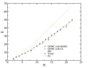
These results show that the pairing is less important in the trial wave function for the finite systems than it is in the uniform gas. While in the homogeneous gas a BCS treatment of the trial function lowers the energy by more than 20 ( and ), the difference in energy between the both phases of the trapped gas does not exceed at the most in the open shell configuration . At the shell closures, the BCS treatment does not offer any improvement
There is a virial theorem for unitary trapped gases given bycastin06 , where . The theory can thus be tested by independently calculating the expectation value of the trapping potential. Expectation values of operators are usually estimated in the GFMC by the expression . Using this estimate of , we find energies somewhat lower than obtained by direct GFMC calculation (see Fig. 1). This could be due to the errors associated with the extrapolation formula for expectation values.
We now examine how well the energies fit the asymptotic theory for large nonuniform systems. The first term in the theory is the Thomas-Fermi (TF) approximation papen05 ; the TF approximation to the trapped unitary Fermi gas is , where is the universal constant relating the energy of the uniform gas to that of the free Fermi gas. Adding a second term in the expansion gives a better description of the energy of the harmonic oscillator energy of the trapped gas in the large limit br97 . We therefore will include that in the fit to the energies, using the form
| (6) |
As it may be seen from Fig. 1, there is also a significant odd-even variation in the energies. We shall include this effect as well by fitting to the function
| (7) |
The result of the fit is shown by the dashed line in Fig. 1. The fit value of is . This is somewhat higher than the bulk value . This suggests that the convergence to the bulk is rather slow. One might expect to see shell effects in the energies once the smooth trends have been taken out. The HO energies, for example, oscillate around with (negative) peaks at the shell closures. The effect is visible in the abrupt change of slop of the HO curve in Fig. 1. However, in our fit to the calculated energies, we do not see a visible shell closure effect. In the fit we find for the parameter the value , in accordance with the average of the odd-even staggering of the energy . If the pairing gap were controlled by the density at the center, it would be much larger; of the order of shell spacing or higher. On the other hand, if the odd particle is most sensitive to the surface region, the pair effect could be smaller. A more systematic approach to LDA exists where the superfluid correlation is introduced bulgac02a ; bulgac02b .
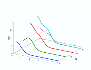
We now turn to the density distributions calculated with the GFMC. We determine the density by binning the values obtained by the Monte Carlo sampling. With paths and 1000 samples per path there is adequate statistics to get details of the density distribution well beyond the mean square radii. Fig. 2 shows the calculated densities for and . We notice that the central densities show a pronounced dip for and a peak for . These are characteristic of shell structure, depending on whether the highest occupied shell has -wave orbitals or not. Fig. 2 also shows the HO density for . The density of the interacting system is more compact, as required by its lower energy and the virial theorem. The central peak has roughly the same relative shape in the two cases. Thus the basic HO pattern is maintained, even though the system shrinks in size.
Let us return again to the problem of the trial function and its fixed nodal structure. It is interesting to ask how different are the nodal positions for the different ’s. We can characterize the trial wave functions by their relative overlaps of the sign domains. If we define
the nodal overlap between and is given as . From this definition, nodal overlap ranges . Because of the strong suppression of the superfluidity at the shell closures the nodal overlap between the normal and the superfluid node wave functions seems to be the largest at the shell closures and has low values at and at .
We believe our computed energy systematics is reliable enough to arrive at the following conclusions. 1) The energies are significantly higher than given by the TF model with bulk . 2) Stabilization of closed shell systems with respect to open shell ones is much weaker than in the free gas. However, the density distribution has pronounced fluctuations similar to those of the pure harmonic oscillator density. 3) There is a substantial pairing visible in the odd-even binding energy differences, but the magnitude is less than the bulk pairing parameter associated with a uniform system of density equal to the central value in the finite system.
We thank A. Bulgac, J. Carlson, M. Forbes, and S. Tan for discussions. This work was supported by the U.S. Department of Energy under Grants DE-FG02-00ER41132 and DE-FC02-07ER41457. Computations were performed in part on the NERSC computer facility.
References
- (1) K. M. O’Hara et al., Science 298, 2179 (2002).
- (2) M. Bartenstein et al., Phys. Rev. Lett. 92, 120401 (2004).
- (3) T. Bourdel et al., Phys. Rev. Lett. 93, 050401 (2004).
- (4) C. Chin et al., Science 305, 1128 (2004).
- (5) M. W. Zwierlein et al., Nature 435, 1047 (2005).
- (6) J. Kinast et al., Science 307, 1296 (2005).
- (7) J. T. Stewart, J. P. Gaebler, C. A. Regal, and D. S. Jin, Phys. Rev. Lett. 97, 220406 (2006).
- (8) J. Carlson, S.Y. Chang, V.R. Pandharipande, and K.E. Schmidt, Phys. Rev. Lett. 91 050401 (2003).
- (9) M. H. Kalos et al, Phys. Rev. A 9 2178 (1974).
- (10) H. Heiselberg and B. Mottelson, Phys. Rev. Lett. 88 190401 (2002).
- (11) G.M. Bruun and H. Heiselberg, Phys. Rev. A65 053407 (2002).
- (12) F. Werner and Y. Castin, Phys. Rev. Lett. 97 150401 (2006).
- (13) F. Werner and Y. Castin, Phys. Rev. A 74 053604 (2006).
- (14) T. Papenbrock, Phys. Rev. A 72 041603(R) (2005).
- (15) M. Brack, R. Bhaduri and R. K. Bhaduri, “Semiclassical Physics”, (Addison-Wesley, Reading, 1997).
- (16) Y. Yu and A. Bulgac, Phys. Rev. Lett. 90, 222501 (2003).
- (17) A. Bulgac, Phys. Rev. C 65, 051305(R) (2002).