Impedance Calculations of Non-Axisymmetric
Transitions Using the Optical Approximation

Abstract

In a companion report, we have derived a method for finding the impedance at high frequencies of vacuum chamber transitions that are short compared to the catch-up distance, in a frequency regime that—in analogy to geometric optics for light—we call the optical regime. In this report we apply the method to various non-axisymmetric geometries such as irises/short collimators in a beam pipe, step-in transitions, step-out transitions, and more complicated transitions of practical importance. Most of our results are analytical, with a few given in terms of a simple one dimensional integral. Our results are compared to wakefield simulations with the time-domain, finite-difference program ECHO, and excellent agreement is found.

Submitted to Physical Review Special Topics–Accelerators and Beams

I Introduction

In many current and future accelerator projects short, intense bunches of charged particles are transported through vacuum chambers that include objects such as transitions, irises, and collimators. For example, in the beam delivery system of the International Linear Collider (ILC) 3 nC, 300 $\mu$m-long bunches encounter many collimators on their way to the interaction region ILC . Or, in the undulator region of the Linac Coherent Light Source (LCLS) a 1 nC, 20 $\mu$m-long bunch passes by square-to-round transitions, bpm’s, and other changes in chamber geometry LCLS . Wakefields generated by such changes in vacuum chamber geometry can negatively affect the beam emittance and ultimately the performance of an accelerator. Numerically obtaining the strength of the wakefields or, equivalently, of the impedances for short bunches in such vacuum chamber objects can be difficult, in particular when the object is long and non-cylindrically symmetric.

In a recent paper Stupakov07 we developed a method to solve such seemingly difficult problems in a so-called optical approximation. This method is valid in the limit of high frequencies and reduces the calculation of the impedance to the two dimensional integration of potential functions. In this report we make use of this method to work out solutions to a selection of 3D (shorthand for non-cylindrically symmetric) geometries that can be encountered in today’s accelerators.

The geometry of the problems to be considered is, in general, of the type sketched in Fig. 1. An in-going beam pipe (region $A$ with cross-section profile $S_{A}$) is followed by a short transition (the gap or aperture region $G$ with cross-section $S_{G}$) and ends in an out-going pipe (region $B$ with cross-section $S_{B}$). We limit consideration to cases where $S_{G}$ is contained within the intersection of $S_{A}$ and $S_{B}$ [$S_{G}\subseteq(S_{A}\cap S_{B})$]. The transition need not be smooth like the one in the figure. A speed of light beam passes through the three regions on a straight line that we call the design orbit. At first there is no assumption on transverse symmetry in the three region. However, we do assume that the axes of regions $A$ and $B$ are parallel to the design orbit. Note that if $S_{G}=S_{B}$ the structure is called a step-in transition (by which we mean a short, inward transition), if $S_{G}=S_{A}$ it is a step-out transition (a short, outward transition). If $S_{A}=S_{B}$, with the aperture of $S_{G}$ smaller than the beam pipes, then the structure is an iris (a metallic diaphragm with a hole or slot) or short collimator in a beam pipe.

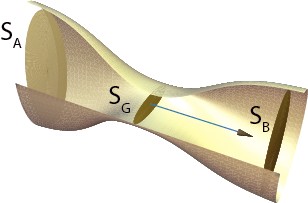
Figure 1: Sketch of a generalized 3D transition, showing the regions $A$, $G$, and $B$, with cross-sections $S_{A}$, $S_{G}$, and $S_{B}$, respectively.

We are interested in finding the high frequency longitudinal or transverse impedance of a general transition such as is sketched in Fig. 1. The impedance regime can be described as the regime of geometric optics. This regime is applicable provided that (1) the frequency is high and (2) the transition is short. By condition (1), we mean that the frequency $\omega\gg c/g$, with $c$ the speed of light and $g$ the minimum aperture of the structure. If the transition is tapered, we require further that $\omega\gg c/(g\theta)$, with $\theta$ the taper angle. By condition (2), we mean that the length of the transition is short compared to the catch-up distance, $\ell=g^{2}\omega/c$. Note that in the optical regime the high frequency longitudinal impedance of a structure is resistive, with the impedance $Z_{\parallel}$ real and independent of frequency. The transverse impedance $Z_{\perp}$ is also real and depends on frequency as $\omega^{-1}$.

The method of Ref. Stupakov07 can be used to find the impedance, for example, for an iris in a beam pipe, a step-in or step-out transition, and a short collimator. Also, there are objects that we call long collimators; i.e. collimators that have a fixed (minimum) aperture over a length that is long compared to the catch-up distance $\ell$, with transitions at the front and back ends. For long collimators our methods also apply, provided that the two transitions satisfy the above two conditions. For such a collimator the impedance is the sum of the impedances of its two transitions. Note, however, that for intermediate length collimators, those of length comparable to the catch-up distance, our methods do not apply.

In Ref. Stupakov07 the impedance of a general transition in the optical regime is developed following a systematic approach. Earlier work on the subject was focused on specific geometries and often was rather informal in nature. Balakin and Novokhatski were among the first to address the question of impedance in the optical regime Novokhatski . Heifets and Kheifets studied the longitudinal impedance of round step-in and step-out transitions (in the optical regime) numerically by field matching Heifets . For round, long collimators the dipole mode impedance was obtained rigorously in Ref. Palumbo , and the higher azimuthal mode impedances, more informally, in Ref. Zimmermann . The impedance of short and long, round and 3D collimators was studied numerically in Refs. Zagorodnov06 , BaneZ06 ; it was found, for example, that the impedances of short and long collimators, in general, differ significantly in amplitude (by a factor $\sim 2$ in the round, transverse case).

The impedances that we obtain in this report following our method will also be compared to numerical results obtained by the computer program ECHO ECHO . This program solves Maxwell’s equations to find the wakefield of an ultra-relativistic Gaussian bunch within (perfectly conducting) metallic boundaries of fully 3D geometry. From the wakefields of a sufficiently short bunch the impedance in the optical regime can be obtained directly. In the present report discussions of ECHO calculations will be brief; their main purpose is to confirm our results and to give us confidence in our method.

This report is organized as follows: In Section II the method of calculation, derived in the companion paper, Ref. Stupakov07 , is presented. At the end of this section some details of the ECHO simulations will be given. The heart of the present report, however, is the next four sections where our method is applied to 3D transition examples. The problems that we solve are example irises or short collimators within a beam pipe (Section III), step-in transitions (Section IV), step-out transitions (Section V), and more complicated transitions (Section VI). In these sections our results will be compared briefly to ECHO simulation results. Section VII gives the conclusions. In the Appendix specific limits for the impedance of an elliptical step-out transition are derived. Note that although we follow the method of Ref. Stupakov07 in this report, the notation used here is not exactly the same. Note also that Gaussian units will be used throughout; to convert impedances to MKS units, one multiplies by the factor $Z_{0}c/4\pi$, with $Z_{0}=377$ $\Omega$.

II Impedance Calculations

Consider a general (transversely non-symmetric) transition. Let the design orbit follow the $z$-axis, with the particle motion in the $+z$ direction. The transverse impedance of a general transition consists of monopole, dipole, and quadrupole components (with respect to the design orbit) that involve tensors, and the method of Ref. Stupakov07 can, in principle, deal with such problems. However, to simplify, in this report we will limit consideration to geometries for which the design orbit lies on a vertical symmetry plane of the boundaries, defined by (horizontal coordinate) $x=0$. Then the transverse (vertical, $y$) impedance (with respect to the reference trajectory) can be written as

$$Z_{\perp,tot}=Z_{\perp,m}+y_{1}Z_{\perp,d}+y_{2}Z_{\perp,q}\ ,$$ (1)

where the three terms are called the (transverse) monopole, dipole, and quadrupole contributions; where $y_{1}$ is a small offset of particle 1 (the leading particle), and $y_{2}$ a small offset of particle 2 (the trailing particle, see Fig. 2). Note that the horizontal impedance has an equation equivalent to Eq. (1), with the quadrupole term equal to $(-Z_{\perp,q})$.

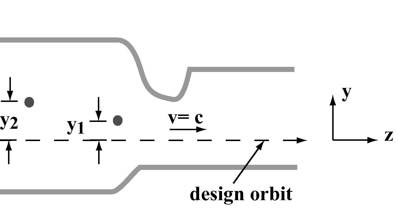
Figure 2: Sketch of a transition showing the relationship of the design trajectory and the vertical offsets of particle 1, $y_{1}$, and particle 2, $y_{2}$ (the particles are indicated by red dots). For the calculations the offsets $y_{1}$, $y_{2}$, are assumed to be small.

For most of the examples of this paper, the system has also a horizontal symmetry plane and the design orbit lies in this plane. In such a case $Z_{\perp,m}=0$; if, in addition, $y_{1}=y_{2}=y_{0}$ we can define a normalized total impedance

$$Z_{\perp}=\frac{Z_{\perp,tot}}{y_{0}}=Z_{\perp,d}+Z_{\perp,q}\ .$$ (2)

By convention, this is the normal definition of total transverse impedance for bi-symmetric problems. (In this paper, however, we will calculate the individual terms $Z_{\perp,d}$ and $Z_{\perp,q}$ as well as $Z_{\perp}$ for bi-symmetric problems.) The transverse wake at position $s$ within a bunch ($s<0$ is toward the head), normalized to the offset $y_{0}$, in the optical regime is given by

$$W_{\perp}(s)=\frac{i}{2\pi}\int_{-\infty}^{\infty}Z_{\perp}(\omega){\tilde{\lambda}_{z}}(\omega)e^{-i\omega s/c}\,d\omega=(\omega Z_{\perp})\int_{-\infty}^{s}\lambda_{z}(s^{\prime})\,ds^{\prime}\ ,$$ (3)

with ${\tilde{\lambda}_{z}}(\omega)$ the Fourier transform of the line charge density $\lambda_{z}(s)$. To arrive at the last expression in this equation we have used the fact that, in the optical regime, $Z_{\perp}\propto\omega^{-1}$. Thus the quantity $(\omega Z_{\perp})$ is independent of frequency. The result is proportional to the integral of the line charge density (and in the longitudinal case, it is proportional to the line charge density itself). The kick factor $\kappa_{\perp}$, the average kick experienced by the beam per unit charge per unit offset, is the integral of $W_{\perp}(s)$ when weighted by the longitudinal charge density. In the optical regime the kick factor is simply given by the constant

$$\kappa_{\perp}=\frac{(\omega Z_{\perp})}{2}\ .$$ (4)

In Ref. Stupakov07 using the Panofsky-Wenzel theorem Panofsky56 , the transverse monopole, dipole, and quadrupole terms are related to longitudinal monopole, dipole, and quadrupole impedances:

$$Z_{\perp,m}=\frac{c}{\omega}Z_{\parallel,m}\ ,\quad\quad Z_{\perp,d}=\frac{c}{\omega}Z_{\parallel,d}\ ,\quad\quad Z_{\perp,q}=\frac{2c}{\omega}Z_{\parallel,q}\ .$$ (5)

The longitudinal impedances can, in turn, be obtained from integrals involving the Green functions to Poisson’s equation (the potentials) in regions $A$ and $B$ of the transition of interest. In the case of the monopole part

$$Z_{\parallel,m}=\frac{1}{2\pi c}\left[\int_{S_{B}}\nabla\varphi_{m,B}\cdot\nabla\varphi_{d,B}\,dS-\int_{S_{G}}\nabla\varphi_{m,A}\cdot\nabla\varphi_{d,B}\,dS\right]\ ,$$ (6)

with the integrals taken over the cross-section areas $S_{B}$ and $S_{G}$, respectively. Here the monopole and quad potentials in region $A$ are given by the solutions to

$$\nabla^{2}\varphi_{m,A}=-4\pi\delta(y)\delta(x)\ ,\quad\quad\nabla^{2}\varphi_{d,A}=4\pi\delta^{\prime}(y)\delta(x)\ ,$$ (7)

with boundary conditions $\varphi_{m,A}=0$, $\varphi_{d,A}=0$, on metallic boundary $C_{A}$ that encloses $S_{A}$. Similar equations hold for $\varphi_{m,B}$ and $\varphi_{d,B}$ of region $B$.

In the case of the dipole part of the impedance

$$Z_{\parallel,d}=\frac{1}{2\pi c}\left[\int_{S_{B}}(\nabla\varphi_{d,B})^{2}\,dS-\int_{S_{G}}\nabla\varphi_{d,A}\cdot\nabla\varphi_{d,B}\,dS\right]\ .$$ (8)

For the quad part of impedance

$$Z_{\parallel,q}=\frac{1}{2\pi c}\left[\int_{S_{B}}\nabla\varphi_{m,B}\cdot\nabla\varphi_{q,B}\,dS-\int_{S_{G}}\nabla\varphi_{m,A}\cdot\nabla\varphi_{q,B}\,dS\right]\ .$$ (9)

The quadrupole potential in region $B$ is given by the solution to

$$\nabla^{2}\varphi_{q,B}=-2\pi\delta^{\prime\prime}(y)\delta(x)\ ,$$ (10)

with $\varphi_{q,B}=0$ on boundary $C_{B}$. Finally, the longitudinal impedance on the reference trajectory is given by:

$$Z_{\parallel,long}=\frac{1}{2\pi c}\left[\int_{S_{B}}(\nabla\varphi_{m,B})^{2}\,dS-\int_{S_{G}}\nabla\varphi_{m,A}\cdot\nabla\varphi_{m,B}\,dS\right]\ .$$ (11)

To obtain the needed potentials $\varphi_{m}$, $\varphi_{d}$, $\varphi_{q}$, we begin with the Green function solution to

$$\nabla^{2}G(x,y,y_{0})=-4\pi\delta(x)\delta(y-y_{0})\ ,$$ (12)

where $G=0$ on the boundary $C$ of the surface of interest $S$. Here the source particle is located at $x=0$, $y=y_{0}$. For region $S$, $\varphi_{m}(x,y)=G(x,y,0)$,

$$\varphi_{d}(x,y)=\left[\frac{\partial}{\partial y_{0}}G(x,y,y_{0})\right]_{y_{0}=0}\ ,\quad\ \varphi_{q}(x,y)=\frac{1}{2}\left[\frac{\partial^{2}}{\partial y_{0}^{2}}G(x,y,y_{0})\right]_{y_{0}=0}\ .$$ (13)

As was shown in Ref. Stupakov07 , with the help of Green’s first identity Green ,

$$\int_{S}(\phi\nabla^{2}\psi+\nabla\phi\cdot\nabla\psi)\,dS=\int_{C}\phi{\bf n}\cdot{\mathbf{\nabla}}\psi\,dl\ ,$$ (14)

the surface integrals involved in the impedance equations can be converted to line integrals. In this formula $\phi$ and $\psi$ are functions that can be differentiated twice; $S$ is a surface over which a surface integration is performed; $C$ is the contour that encloses $S$ and over which a line integral is performed; and ${\bf n}$ is a unit normal vector pointing outward from the contour. This device is used throughout the examples of this report.

Numerical Comparisons

A great number of ECHO simulations were performed to test and verify our results. ECHO is a 3D, time-domain finite difference program that calculates wakefields generated by an ultra-relativistic bunch passing through the structure. ECHO has two features that make these 3D, optical regime simulations tractable. (1) A method to reduce the so-called “mesh dispersion”—errors generated in time-domain mesh programs that are especially difficult to deal with for the combination of short bunches and long structures. (2) An indirect method of calculating wakes in 3D structures that eliminates long downstream beam pipes, which would be needed in the case of direct wake calculation with very short bunches. Since the ECHO simulations play a supporting role in the present report, other than comparing results, we will only discuss them briefly. For a more detailed report on ECHO, see e.g. Ref. ECHO .

A few comments on the parameters used in the ECHO simulations: The bunches in the simulations are Gaussian. Typically we choose $\sigma_{z}=g/10$, with $g$ the minimum vertical half aperture of the iris or transition. For a flat iris or beam pipe we take the structure half-width $w=10g$. (In this report we use the word flat to mean “having a rectangular cross-section with a small height to width ratio.”) For a small iris in a beam pipe or a transition opening into a large beam pipe, the beam pipe is square with half-height $10g$. We take mesh sizes to be $\frac{1}{5}\sigma_{z}$, $\frac{5}{8}\sigma_{z}$, $\frac{5}{8}\sigma_{z}$, in the longitudinal, horizontal, vertical directions, respectively. Irises have the thickness of one longitudinal mesh size. For bi-symmetric structures ECHO calculates the dipole and quadrupole components of the wakes independently.

To demonstrate the validity of the optical approximation, and how one moves out of the optical regime as the bunch length increases, we consider the problem of a thin round iris of radius $g$ in a round beam pipe of radius $b$. We choose $b/g=4$. We perform ECHO calculations for bunch lengths in the range $\sigma_{z}/g=0.02$ to 4. In Fig. 3 we plot twice the kick factor of our results as function of bunch length. According to Eq. 4, in the optical regime $2k_{\perp}=\omega Z_{\perp}$, which is a number independent of bunch length or frequency. We see that the result of our numerical calculation is fairly constant up until $\sigma_{z}/g\sim 0.2$, after which the validity of the optical approximation starts to break down. In more detail, we give in Fig. 4 the actual wake functions for four example bunch lengths as obtained by ECHO. The (Gaussian) bunch shape, with the head to the left, is indicated by the black dashes. The analytical wake of a Gaussian bunch in a round iris in the optical regime, $W_{\perp}=[1+{\rm erf}(s/\sqrt{2}\sigma_{z})]/g^{2}$, with ${\rm erf}(x)$ the error function, is also given (the red dashes). We see that, although the weighted average of the wake agrees well for $\sigma_{z}/g\sim 0.2$, good agreement between the wakes over $\pm 4\sigma_{z}$ is not obtained until $\sigma_{z}/g\sim 0.04$.

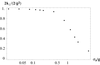
Figure 3: Twice the kick factor $k_{\perp}$ of a thin round iris in a beam pipe vs. rms bunch length $\sigma_{z}$, as obtained by ECHO. The iris radius is $g$.

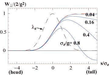
Figure 4: Transverse wake of a thin round iris in a beam pipe as obtained by ECHO. Results for bunch lengths over iris radius $\sigma_{z}/g=0.04$, 0.16, 0.4, and 0.8 are given. The (Gaussian) bunch shape, with the head to the left, is indicated by the black dashes. The analytical wake of a Gaussian bunch in a round iris in the optical regime, $W_{\perp}=[1+{\rm erf}(s/\sqrt{2}\sigma_{z})]/g^{2}$, with ${\rm erf}(x)$ the error function, is also given (the red dashes).

III Iris/Short Collimator in Beam Pipe

We begin by performing calculations of examples with thin irises or short collimators in a beam pipe (for an example, see Fig. 5). In these cases the solution is given by a particularly simple “clipping” type calculation of the energy impinging on the iris wall.

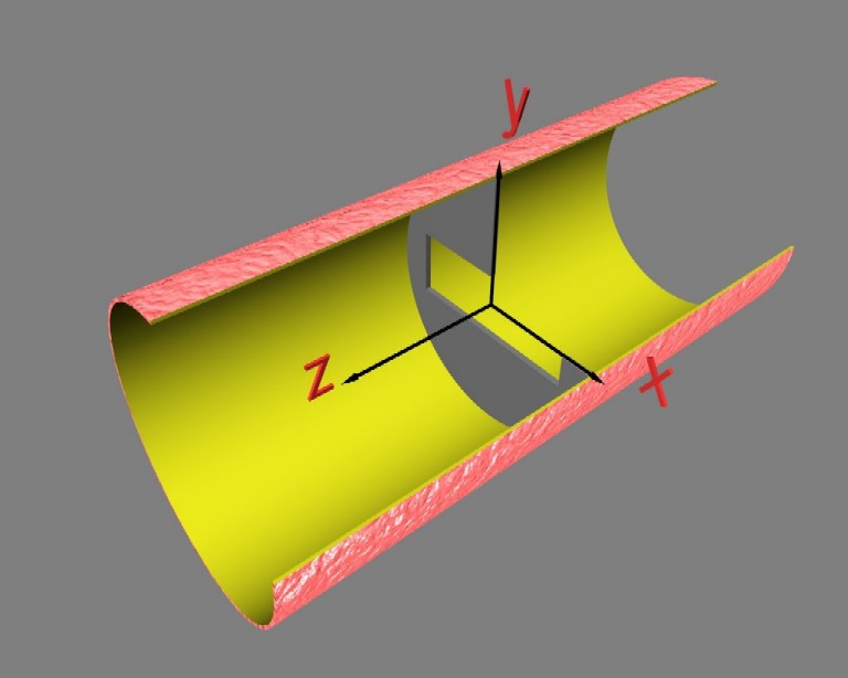
Figure 5: An iris in a beam pipe.

For these examples the beam pipes in Region A and B are identical, i.e. $S_{B}=S_{A}$. Thus Eqs. (5), (8), (9), give

$$Z_{\perp,d}=\frac{1}{2\pi\omega}\int_{S_{B}-S_{G}}(\nabla\varphi_{d,B})^{2}\,dS\ ,$$ (15)

$$Z_{\perp,q}=\frac{1}{\pi\omega}\int_{S_{B}-S_{G}}\nabla\varphi_{m,B}\cdot\nabla\varphi_{q,B}\,dS\ .$$ (16)

Both equations involve integrals over the metallic surface of the iris. Using Green’s first identity and considering the fact that $\nabla\varphi^{2}=0$ in any region that precludes the axis, we can write Eqs. (15), (16), as one dimensional integrals. For example, Eq. (15) becomes

$$Z_{\perp,d}=\frac{1}{2\pi\omega}\int_{C_{G}}\varphi_{d,B}{\bf n}\cdot\nabla\varphi_{d,B}\,dl\ ,$$ (17)

where the integral on the right is a line integral over the curve that encloses the area of $S_{G}$, which we denote by $C_{G}$, and ${\bf n}$ is a unit vector normal to this curve in the direction of the axis (an identical integral over $C_{B}$ was dropped, since $\varphi_{d,B}=0$ on $C_{B}$). Similarly,

$$Z_{\perp,q}=\frac{1}{\pi\omega}\int_{C_{G}}\varphi_{m,B}{\bf n}\cdot\nabla\varphi_{q,B}\,dl\ .$$ (18)

The examples dealt with in this section are: (I1) a small, flat iris (or horizontal slot) in a beam pipe, (I1b) the same but with the design orbit shifted vertically, (I2) a small rectangular iris, (I3) a small elliptical iris, (I4) a flat iris (not necessarily small) in a flat beam pipe. In all cases except I1b, the design orbit is on a horizontal symmetry plane. A cross-section view of the geometries is sketched in Fig. 6. Dimension labels and the design orbit location are also shown.

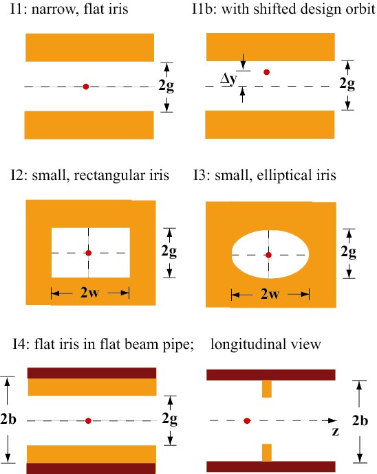
Figure 6: Cross-section views of the iris/short collimator geometries considered in this section (for case I4 a longitudinal view is also given). Dimension labels are given, and the design orbit location is indicated by the red dot. In cases I1-I3 the beam pipe aperture is specified as large compared to the iris aperture; in case I4 the beam pipe is flat, with vertical aperture $2b$. For case I4 two colors are used for the boundaries as an aid in visualization.

In the following subsections (except for subsection I4) we will assume that the pipe radius is very large compared to the iris aperture. We can use the free-space Green function for a particle vertically offset by $y_{0}$:

$$G(x,y,y_{0})=-\ln[x^{2}+(y-y_{0})^{2}]\ .$$ (19)

From this Green function we obtain the potentials:

$$\varphi_{m}=-\ln(x^{2}+y^{2})\ ,\quad\varphi_{d}=\frac{2y}{x^{2}+y^{2}}\ ,\quad\varphi_{q}=\frac{y^{2}-x^{2}}{(x^{2}+y^{2})^{2}}\ .$$ (20)

Then using these potentials, we perform the calculations of Eqs. (17), (18).

The error in transverse impedance introduced by the approximation of the free-space Green function is relatively small. For example, in the case of a round (i.e. cylindrically symmetric) iris of radius $g$ within a round beam pipe of radius $b$ it is known that the correction to the first order term is $(g/b)^{4}$ Zagorodnov06 .

I1. Flat Iris or Horizontal Slot in Large Pipe

Consider a large beam pipe containing an iris with a horizontal slot of vertical size $2g$, with $g$ very small compared to the beam pipe size. We take the reference trajectory to be the symmetry line, so the monopole term $Z_{\perp,m}=0$. The dipole term is given by

$$Z_{\perp,d}=-\frac{2}{\pi\omega}\int_{0}^{\infty}\varphi_{d,B}(x,g)\frac{\partial\varphi_{d,B}}{\partial y}(x,g)\,dx\ ,$$ (21)

and similarly for the quadrupole term. With the free-space potentials the integrals can be performed analytically, and after some algebra we obtain

$$Z_{\perp,d}=Z_{\perp,q}=\frac{1}{\omega g^{2}}\ ,\quad Z_{\perp}=\frac{2}{\omega g^{2}}\ .$$ (22)

We see that the dipole and quad terms are equal, and that the total result is the same as the leading order impedance for a round, thin iris of radius $g$ Zagorodnov06 . Note that for a flat iris that is oriented vertically, we have $Z_{\perp,d}=-Z_{\perp,q}=1/(\omega g^{2})$ and $Z_{\perp}=0$.

I1b. Case of Shifted Design Orbit

We can also find the impedance for the case the design orbit is shifted vertically by $\Delta y$. In this case the (transverse) monopole term $Z_{\perp,m}$ dominates the transverse impedance, and we can neglect the effect of $Z_{\perp,d}$ and $Z_{\perp,q}$ [see Eq. (1)]. The transverse monopole term is obtained using Eqs. (5), (6). Then the calculation proceeds in the same manner as before:

$$Z_{\perp,m} = -\frac{1}{\pi\omega}\int_{0}^{\infty}\left[\varphi_{d,B}(x,g-\Delta y)\frac{\partial\varphi_{m,B}}{\partial y}(x,g-\Delta y)\right.$$

$$\quad\quad\quad+\left.\varphi_{d,B}(x,-g-\Delta y)\frac{\partial\varphi_{m,B}}{\partial y}(x,-g-\Delta y)\right]\,dx\ .$$

We find that the transverse impedance is given by

$$Z_{\perp,m}=\frac{1}{\omega}\left[\frac{1}{g-\Delta y}-\frac{1}{g+\Delta y}\right]\ .$$ (24)

For small $\Delta y$, $Z_{\perp,m}=2\Delta y/(\omega g^{2})$, which is consistent with our earlier results.

I2. Rectangular Iris

For the case of a rectangular iris with a small aperture of $2w$ by $2g$ (horizontal by vertical) the calculation follows the same procedure as before; however, the integration now is a line integral along the rectangular aperture. We perform integrals like

$$Z_{\perp,d}=-\frac{2}{\pi\omega}\left[\int_{0}^{w}\varphi_{d,B}(x,g)\frac{\partial\varphi_{d,B}}{\partial y}(x,g)\,dx+\int_{0}^{g}\varphi_{d,B}(w,y)\frac{\partial\varphi_{d,B}}{\partial x}(w,y)\,dy\right]\ .$$ (25)

The final solution is

$$Z_{\perp,d} = \frac{2}{\pi\omega g^{2}}\frac{\alpha+{\rm arccot}(\alpha)+\alpha^{2}\arctan(\alpha)}{\alpha^{2}}$$

$$Z_{\perp,q} = \frac{2}{\pi\omega g^{2}}\frac{\alpha(-1+\alpha^{2})+(1+\alpha^{2})[{-\rm arccot}(\alpha)+\alpha^{2}\arctan(\alpha)]}{\alpha^{2}(1+\alpha^{2})}$$

$$Z_{\perp} = \frac{4}{\pi\omega g^{2}}\frac{\alpha+(1+\alpha^{2})\arctan(\alpha)}{1+\alpha^{2}}$$ (26)

where $\alpha=w/g$.

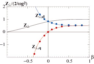
Figure 7: For a rectangular iris in a beam pipe, the transverse impedances $Z_{\perp}$, $Z_{\perp,d}$, $Z_{\perp,q}$, normalized to $2/(\omega g^{2})$, as functions of $\beta=(w-g)/(w+g)$. Plotting symbols give ECHO numerical results.

The results, when normalized to $2/\omega g^{2}$, are plotted as functions of $\beta=(w-g)/(w+g)$ in Fig. 7. Note that when $\beta=1$ the results agree with the results for the iris with the infinitely wide horizontal slot, given above. For $\beta=-1$ (an infinitely high vertical slot) $Z_{\perp,q}=-Z_{\perp,d}=-1/(\omega w^{2})$ and $Z_{\perp}=0$. For the special case of a square aperture $Z_{\perp}=Z_{\perp,d}=2(\frac{1}{\pi}+\frac{1}{2})/g^{2}$ and $Z_{\perp,q}=0$. Note that the horizontal impedance is obtained from Eqs. (26) by exchanging $w$ and $g$.

In Fig. 7 ECHO numerical results for $Z_{\perp,d}$ and $Z_{\perp,q}$ are shown by the plotting symbols. We see good agreement with the results of our method.

I3. Elliptical Iris

The impedance calculation for an elliptical iris with a small aperture, with axes $w$ by $g$ (horizontal by vertical), follows in a similar manner to the rectangular iris case. The equations that need to be solved are Eqs. (17), (18). We see that the elliptical case is more complicated in that it requires the formation of ${\bf n}\cdot\nabla\varphi_{q,B}$ and of the length metric on the ellipse of the iris, though the final solution is quite simple. We find that

$$Z_{\perp,d}=\frac{1}{\omega g^{2}}\left(1+\frac{g^{2}}{w^{2}}\right)\ ,\quad Z_{\perp,q}=\frac{1}{\omega g^{2}}\left(1-\frac{g^{2}}{w^{2}}\right)\ ,\quad Z_{\perp}=\frac{2}{\omega g^{2}}\ .$$ (27)

We find that for an elliptical iris $Z_{\perp}$ is independent of the size of the horizontal axis $w$! As was true for the rectangular iris, the horizontal impedance of the elliptical iris can be obtained by exchanging $w$ and $g$ in the solution equations. In Fig. 8 we plot the analytical results and compare with ECHO numerical results. We see good agreement.

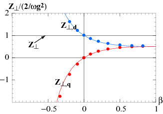
Figure 8: For an elliptical iris in a beam pipe, the transverse impedances $Z_{\perp}$, $Z_{\perp,d}$, $Z_{\perp,q}$, normalized to $2/(\omega g^{2})$, as functions of $\beta=(w-g)/(w+g)$. Plotting symbols give ECHO numerical results.

I4. Flat Iris in Flat Beam Pipe

Consider a flat iris of height $2g$ centered within a flat beam pipe of height $2b$. We begin this problem with the Green function between two parallel plates of aperture $2b$ MorseFeshbach

$$G(x,y,y_{0})=\ln\left[\frac{\cosh\frac{\pi x}{2b}+\cos\frac{\pi(y+y_{0})}{2b}}{\cosh\frac{\pi x}{2b}-\cos\frac{\pi(y-y_{0})}{2b}}\right]\ .$$ (28)

The calculation procedure is the same as for the free-space-to-flat-iris example, Example I1. The potentials are

$$\varphi_{m,B}(x,y) = \ln\left[\frac{\cosh\frac{\pi x}{2b}+\cos\frac{\pi y}{2b}}{\cosh\frac{\pi x}{2b}-\cos\frac{\pi y}{2b}}\right]$$

$$\varphi_{d,B}(x,y) = \frac{\pi}{2b}\,\frac{\sin\frac{\pi y}{b}}{\cosh^{2}\frac{\pi x}{2b}-\cos^{2}\frac{\pi y}{2b}}$$

$$\varphi_{q,B}(x,y) = \frac{\pi^{2}}{8b^{2}}\,\frac{(-2+\cosh\frac{\pi x}{b}+\cos\frac{\pi y}{b})\cosh\frac{\pi x}{2b}\cos\frac{\pi y}{2b}}{\left(\cosh^{2}\frac{\pi x}{2b}-\cos^{2}\frac{\pi y}{2b}\right)^{2}}\ .$$ (29)

The final solution is

$$Z_{\perp,d} = \frac{\pi\alpha^{2}}{2\omega g^{2}}\csc^{2}(\pi\alpha)[2\pi(1-\alpha)+\sin(2\pi\alpha)]$$

$$Z_{\perp,q} = \frac{\pi\alpha^{2}}{\omega g^{2}}\csc(\pi\alpha)[1+\pi(1-\alpha)\cot(\pi\alpha)]$$

$$Z_{\perp} = \frac{\pi\alpha^{2}}{2\omega g^{2}}\csc^{2}(\pi\alpha/2)[\pi(1-\alpha)+\sin(\pi\alpha)]$$ (30)

where $\alpha=g/b$. These curves are plotted in Fig. 9. The round case, with $g$ and $b$, representing, respectively, the radii of the iris and of the beam pipe, $(Z_{\perp})_{round}=2(1/g^{2}-g^{2}/b^{4})/\omega$ Zagorodnov06 , is also shown (the dashes). We note that $Z_{\perp}$ is always close to and larger for the flat than for the round case.

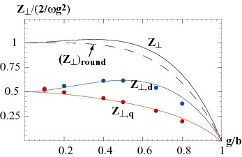
Figure 9: For a flat iris with aperture $2g$ in a flat beam pipe of aperture $2b$, the transverse impedances $Z_{\perp}$, $Z_{\perp,d}$, $Z_{\perp,q}$ as functions of $\alpha=g/b$. Plotting symbols give ECHO numerical results. The round case, $(Z_{\perp})_{round}=2(1/g^{2}-g^{2}/b^{4})/\omega$, is also shown (dashes).

In Fig. 9 ECHO numerical results for $Z_{\perp,d}$ and $Z_{\perp,q}$ are again shown by plotting symbols. We see basically good agreement with the results of our method. We should point out one subtlety however. For $g/b=0.8$ the numerically obtained wake begins to take on some inductive character and the result for impedance begins to deviate from our analytical solution (particularly $Z_{\perp,d}$). We attribute this to the fact that, for the parameters used in the simulations, $(b-g)/b=\sigma_{z}$; as $(b-g)/b\lesssim\sigma_{z}$ we are beginning to leave the optical regime.

Longitudinal Impedance

If we know the geometry of both the beam pipe and the iris we can also obtain the longitudinal impedance, $Z_{\parallel,long}$. For the longitudinal impedance we begin with Eq. (11), which we convert to a line integral, and obtain

$$Z_{\parallel,long} = -\frac{2}{\pi c}\int_{0}^{\infty}\varphi_{m,B}\frac{\partial\varphi_{m,B}}{\partial y}(x,g)\,dx$$ (31)

$$= \frac{8}{c}\int_{0}^{\infty}\frac{\sin\pi\alpha\cosh\pi x}{\cos 2\pi\alpha-\cosh 2\pi x}\ln\left(\frac{\cosh\pi x-\cos\pi\alpha}{\cosh\pi x+\cos\pi\alpha}\right)\,dx\ ,$$

with $\alpha=g/b$. The last integral we evaluate numerically. The result, when normalized to $4/c$, is shown in shown in Fig. 10. For comparison, the round case impedance (with $g$ and $b$ representing, respectively, the iris and beam pipe radius), is also shown. We see that the longitudinal impedance in the flat case is always less than in the round case.

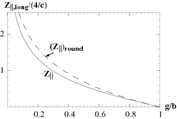
Figure 10: For a thin flat iris with aperture $2g$ in a flat beam pipe of aperture $2b$, the longitudinal impedance $Z_{\parallel,long}$ as function of $\alpha=g/b$. The round case, $(Z_{\parallel})_{round}=4\ln(b/g)/c$, is also shown (dashes).

IV Step-In Transition

For the dipole component of impedance of a step-in transition we replace, in Eq. (8), $S_{G}$ by $S_{B}$, and use Green’s first identity to obtain

$$Z_{\parallel,d} = \frac{1}{2\pi c}\left[\int_{C_{B}}\varphi_{d,B}{\bf n}\cdot{\bf\nabla}\varphi_{d,B}\,dl-\int_{S_{B}}\varphi_{d,B}\nabla^{2}\varphi_{d,B}\,dS\right.$$ (32)

$$\quad\quad\left.-\int_{C_{B}}\varphi_{d,B}{\bf n}\cdot{\bf\nabla}\varphi_{d,A}\,dl+\int_{S_{B}}\varphi_{d,B}\nabla^{2}\varphi_{d,A}\,dS\right]=0$$

The first and third integrals are zero because $\varphi_{d,B}=0$ on boundary $C_{B}$; the second and fourth integrals cancel because the Laplacian is the same independent of region.

The same kind of analysis shows that $Z_{\parallel,q}=0$ in a step-in transition, and that $Z_{\parallel,m}=0$ also in non-symmetric step-in transitions. Since specifics of the geometry were not used in our derivation, we conclude that the total transverse impedance is zero for a (short) step-in transition of any geometry. Similarly the longitudinal impedance of any short step-in transition is also zero in the optical regime (something that has been known to be true for the special case of a round step-in transition Novokhatski , Heifets ). We conclude that the longitudinal and transverse impedance of any step-in transition, in the optical regime, is zero!

The impedance of a long collimator is just the sum of the impedances of a step-in and a step-out transition. Since the impedance of a step-in transition is zero, the impedance of a long collimator is the same as that of a step-out transition alone, the impedance of which we will study in the following section.

V Step-Out Transition

An example step-out transition is sketched in Fig. 11 (the particles move in the $+z$ direction). The examples dealt with in this section are: (T1) a flat beam pipe that transitions to larger flat beam pipe, (T2) a rectangular pipe that transitions to a large pipe, and (T3) an elliptical pipe that transitions to a large pipe. Cross-section views of the geometries (and a longitudinal view in case (T1) are sketched in Fig. 12. Dimension labels and the design orbit location are also shown.

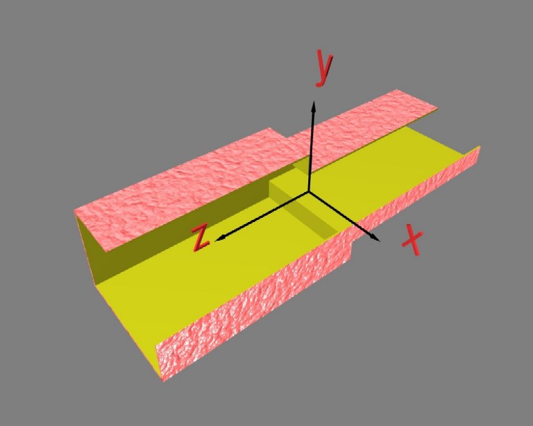
Figure 11: A step-out transition. The particles move in the $+z$ direction.

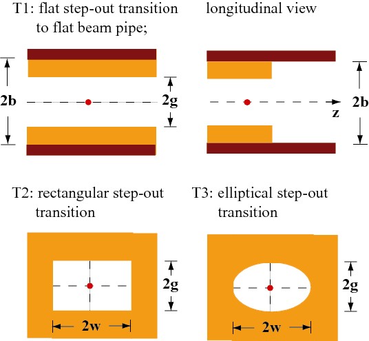
Figure 12: Cross-section views of the step-out transition geometries considered in this section (for case T1 a longitudinal view is also given). Dimension labels are given, and the design orbit location is indicated by the red dot. In cases T2-T3 the outgoing beam pipe aperture is specified as large compared to the incoming beam pipe aperture; in case T1 the outgoing beam pipe is flat, with vertical aperture $2b$. For case T1 two colors are used for the boundaries as an aid in visualization.

For the impedance of a step-out transition we replace, in Eq. (8), $S_{G}$ by $S_{A}$. The impedance function (in the dipole case) $Z_{\parallel,d}$ of a step-out transition can be written, beginning with Eq. (8), as

$$Z_{\parallel,d}=\frac{1}{2\pi c} \left[\int_{S_{B}}(\nabla\varphi_{d,B})^{2}\,dS-\int_{S_{A}}\nabla\varphi_{d,A}\cdot\nabla\varphi_{d,B}\,dS\right]$$

$$=\frac{1}{2\pi c} \left[\int_{S_{B}}(\nabla\varphi_{d,B})^{2}\,dS-\int_{S_{A}}(\nabla\varphi_{d,A})^{2}\,dS\right.$$

$$\left.-\int_{S_{A}}\nabla\varphi_{d,A}\cdot\nabla(\varphi_{d,B}-\varphi_{d,A})\,dS\right]\ .$$ (33)

By using Green’s identity one can easily see that the last integral is zero. Thus

$$Z_{\parallel,d}=\frac{1}{2\pi c}\left[\int_{S_{B}}(\nabla\varphi_{d,B})^{2}\,dS-\int_{S_{A}}(\nabla\varphi_{d,A})^{2}\,dS\right]\ .$$ (34)

This result can be interpreted as $2/c$ times the static field energy of a dipole in region $B$ minus that of a dipole in region $A$. This principle—that the longitudinal impedance (here longitudinal dipole impedance) of a step-out transition in the optical regime is given by twice the difference in the static field energy in the two regions—was first elaborated for the round step-out transition (longitudinal case) by Heifets and Kheifets Heifets . The principle was then used for obtaining higher order wakes (azimuthal mode number $m>0$) of (long) round collimators Zimmermann , and also for specific 3D structures Zagorodnov06 .

We see that a main difference in the calculation of the impedance of a step-out transition and of an iris is that, in the former case the surface integrals are performed over a region that includes the source charges of the potentials, and in the latter case the region of the charges is excluded. In the step-out transition case, however, it turns out that even though the potentials diverge at the source charges, for the impedance two terms with the same divergence are subtracted, and the impedance is finite.

By regrouping integrals and using Green’s identity we can write the impedance of a step-out transition in terms of a simple line integral. The impedance function (for example, in the dipole case) can be written, beginning with Eq. (8), as

$$Z_{\parallel,d}=\frac{1}{2\pi c} \left[\int_{S_{B}-S_{A}}(\nabla\varphi_{d,B})^{2}\,dS-\int_{S_{A}}\nabla\varphi_{d,B}\cdot\nabla(\varphi_{d,A}-\varphi_{d,B})\,dS\right]$$

$$=\frac{1}{2\pi c} \left[\int_{C_{B}-C_{A}}\varphi_{d,B}{\bf n}\cdot\nabla\varphi_{d,B}\,dl-\int_{S_{B}-S_{A}}\varphi_{d,B}\nabla^{2}\varphi_{d,B}\,dS\right.$$

$$\left.-\int_{C_{A}}\varphi_{d,B}{\bf n}\cdot\nabla(\varphi_{d,A}-\varphi_{d,B})\,dl+\int_{S_{A}}\varphi_{d,B}\nabla^{2}(\varphi_{d,A}-\varphi_{d,B})\,dS\right]$$

$$\!\!\!\!\!\!\!\!\!\!\!\!\!\!\!\!\!\!=-\frac{1}{2\pi c}\int_{C_{A}}\varphi_{d,B}{\bf n}\cdot\nabla\varphi_{d,A}\,dl\ .$$ (35)

To go from the second to the third form of the impedance in this equation, we use the fact that $\varphi_{d,B}=0$ on $C_{B}$, that $\nabla^{2}\varphi_{d,B}=0$ in the region $S_{B}-S_{A}$, and that $\nabla^{2}(\varphi_{d,A}-\varphi_{d,B})=0$ everywhere.

However, we can obtain formulas for the impedance of a step-out transition that are even simpler. The dipole part of the impedance, for example, can be written as

$$Z_{\parallel,d} = \frac{1}{2\pi c}\left[\int_{C_{B}}\varphi_{d,B}{\bf n}\cdot{\bf\nabla}\varphi_{d,B}\,dl-\int_{S_{B}}\varphi_{d,B}\nabla^{2}\varphi_{d,B}\,dS\right.$$ (36)

$$\quad\quad\left.-\int_{C_{A}}\varphi_{d,A}{\bf n}\cdot{\bf\nabla}\varphi_{d,B}\,dl+\int_{S_{A}}\varphi_{d,A}\nabla^{2}\varphi_{d,B}\,dS\right]\ .$$

The line integrals are zero again. Combining the remaining terms and substituting for $\nabla^{2}\varphi$ from Eq. (7), we obtain

$$Z_{\perp,d}=\lim_{x,y\to 0}\frac{2}{\omega}\frac{\partial}{\partial y}\left[\varphi_{d,B}(x,y)-\varphi_{d,A}(x,y)\right]\ .$$ (37)

Both dipole potential terms diverge in the limit $x,y\to 0$; however, the divergences are the same, and $Z_{\perp,d}$ is finite.

For the quad component of impedance of a step-out transition we replace, in Eq. (9), $S_{G}$ by $S_{A}$, and use Green’s first identity to obtain

$$Z_{\parallel,q}=\frac{1}{2\pi c}\left[-\int_{S_{B}}\varphi_{q,B}\nabla^{2}\varphi_{m,B}\,dS+\int_{S_{A}}\varphi_{m,A}\nabla^{2}\varphi_{q,B}\,dS\right]\ ,$$ (38)

where the line integral terms are again zero. Substituting for the Laplacians from Eqs. (7), (10), using the relation $\lim_{x,y\to 0}[\partial^{2}\varphi_{m,A}(x,y)/\partial y^{2}-2\varphi_{q,A}(x,y)]=0$, and going to $Z_{\perp,q}$ we obtain

$$Z_{\perp,q}=\lim_{x,y\to 0}\frac{4}{\omega}\left[{\varphi_{q,B}(x,y)}-{\varphi_{q,A}(x,y)}\right]\ .$$ (39)

Similarly, the transverse monopole impedance is

$$Z_{\perp,m}=\lim_{x,y\to 0}\frac{2}{\omega}\left[{\varphi_{d,B}(x,y)}-{\varphi_{d,A}(x,y)}\right]\ ;$$ (40)

the longitudinal impedance is given by

$$Z_{\parallel,long}=\lim_{x,y\to 0}\frac{2}{c}\left[{\varphi_{m,B}(x,y)}-{\varphi_{m,A}(x,y)}\right]\ .$$ (41)

We see that, once the Green functions are known, obtaining the impedances of step-out transitions (as well as long collimators) is a relatively straightforward matter. Whereas an equation of the form Eq. (34) can be interpreted to mean that the longitudinal impedance in the optical regime is $2/c$ times the static field energy of a charge distribution in region $B$ minus that of one in region $A$, these simpler equations can be interpreted to mean that the longitudinal impedance is $2/c$ times the potential difference at the charge distribution in region $B$ minus that at the charge in region $A$.

As was the case with the irises/short collimators, for a transition into a large beam pipe, one also doesn’t need to know details of the large beam pipe in order to calculate the leading order behavior of a transverse impedance. In the equations for impedance one can take the potentials in region $B$ to be derived from the free-space Green function, given in Eq. (19).

T1. Flat Transition

In the case of a flat, symmetric, step-out transition going from aperture $2g$ to $2b$, we substitute the potentials Eqs. (29) into Eqs. (37), (39). We obtain

$$Z_{\perp}=\frac{\pi^{2}}{2\omega}\left(\frac{1}{g^{2}}-\frac{1}{b^{2}}\right)\ ,$$ (42)

with $Z_{\perp,q}=\frac{1}{2}Z_{\perp,d}$. We see thus that the transverse impedance of a flat step-out transition (or of a long, flat collimator) is a factor $\pi^{2}/8$ times the transverse impedance of a long, round collimator, if we take the half-heights in the former case to be equal to the radii in the latter Palumbo . In Fig. 13 we plot the theoretical dependence and compare with ECHO numerical results (the plotting symbols). We see that the agreement is very good.

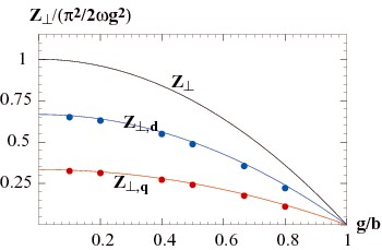
Figure 13: For a step-out transition from a flat pipe of aperture $2g$ into a flat pipe of aperture $2b$, the transverse impedances $Z_{\perp}$, $Z_{\perp,d}$, $Z_{\perp,q}$ as functions of $\alpha=g/b$. Plotting symbols give ECHO numerical results for comparison.

If we perform the longitudinal impedance calculation for the flat step-out transition we find that $Z_{\parallel,long}=4\ln(b/g)/c$, which is the same as for the round case, if we take the half-heights in the flat case to be equal to the radii in the round one.

For a design orbit that is shifted by $\Delta y$ from the symmetry axis, we find, using Eq. (40),

$$Z_{\perp,m}=\frac{\pi}{\omega}\left[\frac{1}{g}\tan\frac{\pi\Delta y}{2g}-\frac{1}{b}\tan\frac{\pi\Delta y}{2b}\right]\ .$$ (43)

Note that for a beam close to the wall at e.g. $y=g$, $Z_{\perp,m}=2/[\omega(g-\Delta y)]$, which is twice as large is we found for the close-to-the-wall impedance in the case of an iris (see Eq. (24)).

T2. Rectangular Transition

Consider a rectangular pipe of width $2w$ and height $2g$ that transitions into a large beam pipe, and a design orbit that follows the symmetry line of the rectangular pipe. The Green’s function for Poisson’s equation in a rectangular pipe has been obtained by Gluckstern, et al Gluckstern . Their result is:

$$G(x,y,y_{0}) =-4\sum_{n=1}^{\infty}\frac{e^{-\frac{n\pi w}{2g}}\cosh\frac{n\pi x}{2g}}{n\cosh\frac{n\pi w}{2g}}\sin\frac{n\pi}{2g}(y+g)\sin\frac{n\pi}{2g}(y_{0}+g)$$

$$+\ln\left\{\left[x^{2}+(y-y_{0})^{2}\right]\frac{\sinh^{2}\frac{\pi x}{4g}+\cos^{2}\frac{\pi}{4g}(y+y_{0})}{\sinh^{2}\frac{\pi x}{4g}+\sin^{2}\frac{\pi}{4g}(y-y_{0})}\right\}$$

$$-\ln\left[{x^{2}+(y-y_{0})^{2}}\right]\ .$$ (44)

The last term contains the singularity. The other terms are everywhere finite, and the sum in the first term converges well.

For our calculation we take region $B$ to have the free space Green function, i.e. the same as the last term in Eq. (44). Thus we have no singularities left in our impedances, since they all involve the difference of potentials in the two regions. Our final result is

$$Z_{\perp,d} = \frac{\pi^{2}}{3\omega g^{2}}\left[1+24\sum_{m=1}^{\infty}\frac{m}{1+e^{2\pi m\alpha}}\right]\ ,$$

$$Z_{\perp,q} = \frac{\pi^{2}}{6\omega g^{2}}\left[1-24\sum_{m=1}^{\infty}\frac{2m-1}{1+e^{\pi(2m-1)\alpha}}\right]\ ,$$ (45)

with $\alpha=w/g$. We perform the sums numerically. The results, when normalized to $\pi^{2}/(2\omega g^{2})$, are plotted as functions of $\beta=(w-g)/(w+g)$ in Fig. 14 ($Z_{\perp}=Z_{\perp,d}+Z_{\perp,q}$). Note that when $\beta=1$ the results agree with the leading order behavior for the flat transition, given above. For $\beta=-1$ (a step-out transition from an infinitely high vertical beam pipe) $Z_{\perp,q}=-Z_{\perp,d}=-\pi^{2}/(6\omega w^{2})$ and $Z_{\perp}=0$. For the special case of a square beam pipe $Z_{\perp}=Z_{\perp,d}=(0.697)\pi^{2}/(2\omega g^{2})$, which is 86% of the result for a round pipe with radius $g$, $4/(\omega g^{2})$; and $Z_{\perp,q}=0$. The plotting symbols in the figure give ECHO numerical results, and we see good agreement. Finally, note that the horizontal impedance is obtained from Eqs. (45) by exchanging $w$ and $g$.

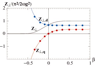
Figure 14: For a rectangular step-out transition to a large beam pipe, the leading order dependence of the transverse impedances $Z_{\perp}$, $Z_{\perp,d}$, $Z_{\perp,q}$, normalized to $\pi^{2}/(2\omega g^{2})$, as functions of $\beta=(w-g)/(w+g)$. The plotting symbols give ECHO numerical results for comparison.

T3. Elliptical Transition

Consider an elliptical pipe of horizontal axis $w$ and vertical axis $g$ that transitions into a large beam pipe, and a design orbit that follows the symmetry line of the elliptical pipe. The Green’s function for Poisson’s equation in an elliptical pipe has been obtained by Gluckstern, et al Gluckstern . For the case $w\geq g$ it is given by

$$G(x,y,y_{0}) =-4\sum_{n=1}^{\infty}\frac{e^{-nu_{0}}}{n}\left[\frac{{\rm Re}T_{n}(\frac{x+iy}{d})\,{\rm Re}T_{n}(\frac{iy_{0}}{d})}{\cosh nu_{0}}+\frac{{\rm Im}T_{n}(\frac{x+iy}{d})\,{\rm Im}T_{n}(\frac{iy_{0}}{d})}{\sinh nu_{0}}\right]$$

$$-\ln\left[{x^{2}+(y-y_{0})^{2}}\right]\ ,$$ (46)

with $T_{n}$ the Chebyshev polynomials of the first kind, $d^{2}=w^{2}-g^{2}$, and $u_{0}={\rm arccoth}\,(w/g)$. [Note that $G$, as given here, is not zero but constant on the elliptical boundary, a fact, however, that does not affect our results.] The calculation procedure is the same as for the rectangular step-out transition. In the elliptical case we find that

$$\hat{\varphi}_{d}(x,y) =8\sum_{m=1}^{\infty}\frac{(-1)^{m}{\rm Im}\left[T_{2m-1}(\frac{x+iy}{d})\right]}{e^{2(2m-1)u_{0}}-1},$$

$$\hat{\varphi}_{q}(x,y) =-4\sum_{m=1}^{\infty}\frac{(-1)^{m}{\rm Re}\left[T_{2m}(\frac{x+iy}{d})\right]}{e^{4mu_{0}}+1},$$ (47)

with $\hat{\varphi}$ signifying the part of the potential that does not contain the singularity. Note that the horizontal ($x$) impedance of a step-out transition is equal to the (vertical) impedance of the transition after it has been rotated by $90^{\circ}$. Thus to obtain the impedances for an elliptical step-out transition with $w<g$ we calculate the $x$ impedances for the rotated case, following the analogous procedure to what we use for finding the $y$ impedances.

We finally obtain

$$Z_{\perp,d} =\frac{16}{\omega g^{2}(\alpha^{2}-1)}\sum_{m=1}^{\infty}\frac{2m-1}{\left(\frac{\alpha+1}{\alpha-1}\right)^{2m-1}-1}\ ,$$

$$Z_{\perp,q} =\frac{32}{\omega g^{2}(\alpha^{2}-1)}\sum_{m=1}^{\infty}\frac{m}{\left(\frac{\alpha+1}{\alpha-1}\right)^{2m}+1}\ ,$$ (48)

with $\alpha=w/g$ (valid for all $\alpha$). We have simplified the results by using the relation $e^{2u_{0}}=(\alpha+1)/|\alpha-1|$. The sums are performed numerically. The results are plotted as functions of $\beta=(w-g)/(w+g)$ in Fig. 15. The plotting symbols in the figure give ECHO numerical results, and we see good agreement. We see that we obtain the expected results for the round case ($\beta=0$), $Z_{\perp,d}=4/(\omega g^{2})$ and $Z_{\perp,q}=0$; for the flat case ($\beta=1$), $Z_{\perp,d}=2Z_{\perp,q}=\pi^{2}/(3\omega g^{2})$. For the case of a horizontally infinitesimally narrow elliptical pipe ($\beta=-1$) we find that $Z_{\perp,d}\approx-Z_{\perp,q}=1/(\omega w^{2})$, and that the total impedance $Z_{\perp}=2/(\omega g^{2})$. Note that in this limit $Z_{\perp}$ has the same value as we obtained for any small elliptical iris in a beam pipe (see Eq. (27)). Details of how all three limits are arrived at can be found in the Appendix.

Figure 15: For an elliptical step-out transition to a large beam pipe, the leading order dependence of the transverse impedances $Z_{\perp}$, $Z_{\perp,d}$, $Z_{\perp,q}$, normalized to $\pi^{2}/(2\omega g^{2})$, as functions of $\beta=(w-g)/(w+g)$. The plotting symbols give ECHO numerical results for comparison.

VI More Complicated Transitions

In this section we give two examples that are neither an iris/short collimator in a beam pipe, nor a step-in or step-out transition. The examples are: (U1)–misaligned flat beam pipes, and (U2)–LCLS-type rectangular-to-round transitions. See Fig. 16. A cut-away perspective view of a pair of the LCLS transitions is also given in Fig. 17.

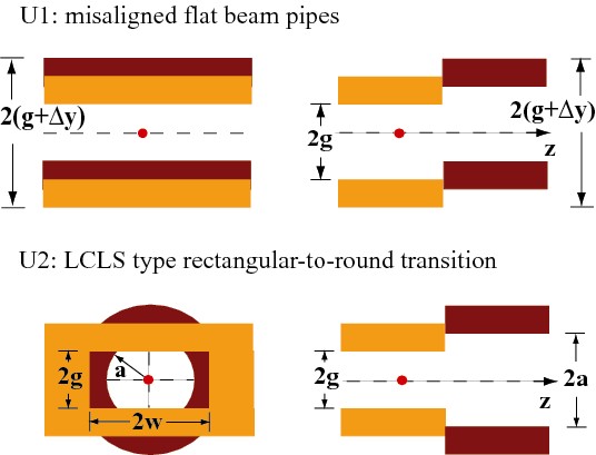
Figure 16: Cross-section view (from upstream end; left figures) and longitudinal view (right figures) of more complicated transitions: U1–misaligned flat pipes, and U2–LCLS-type rectangular-to-round transitions. Dimension labels are given; the design orbit location is indicated by the red dot. Two colors are used as an aid in visualization.

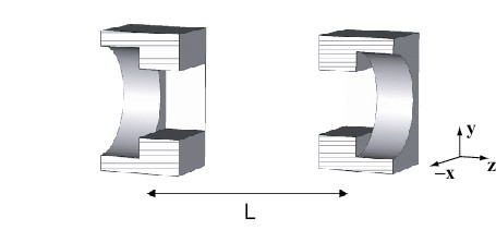
Figure 17: A matching pair of LCLS rectangular-to-round transitions in cut-away perspective view. The distance $L$ between transitions is much larger than the catch-up distance for the nominal bunch length.

U1. Misaligned Flat Beam Pipes

Consider first two flat beam pipes with thick walls and aperture $2g$ that are perfectly aligned and joined at $z=0$. The design orbit lies in the horizontal symmetry plane. Now imagine shifting the $z>0$ pipe vertically by $\Delta y$ ($|\Delta y|<g$) and the $z<0$ pipe by $-\Delta y$, and keeping the design orbit unchanged. Note that the resulting transition no longer has a horizontal symmetry plane.

Let us sketch out the calculation of the transverse impedance $Z_{\perp,m}$ for this structure (for $\Delta y>0$). The potentials for this problem are given by

$$\varphi_{m,A}(x,y) =G(x,y+\Delta y,\Delta y)\ ,\quad\varphi_{d,A}(x,y)=\left.\frac{\partial G}{\partial y_{0}}(x,y+\Delta y,y_{0})\right|_{y_{0}=\Delta y}\ ,$$

$$\varphi_{m,B}(x,y) =G(x,y-\Delta y,-\Delta y)\ ,\quad\varphi_{d,B}(x,y)=\left.\frac{\partial G}{\partial y_{0}}(x,y-\Delta y,y_{0})\right|_{y_{0}=-\Delta y}\ ,$$ (49)

with the flat pipe Green function $G(x,y,y_{0})$ given by Eq. (28), but with $b$ replaced by $g$. Note that, for this geometry, the aperture $S_{G}$ is the intersection of $S_{A}$ and $S_{B}$.

Beginning with Eq. (6), and using Green’s identity, we obtain

$$Z_{\parallel,m} = \frac{1}{2\pi c}\left[\int_{C_{B}}\varphi_{d,B}{\bf n}\cdot\nabla\varphi_{m,B}\,dl-\int_{S_{B}}\varphi_{d,B}\nabla^{2}\varphi_{m,B}\,dS\right.$$ (50)

$$-\left.\int_{C_{G}}\varphi_{d,B}{\bf n}\cdot\nabla\varphi_{m,A}\,dl+\int_{S_{G}}\varphi_{d,B}\nabla^{2}\varphi_{m,A}\,dS\right]\ .$$

The first integral above is zero, because $\varphi_{d,B}$ is zero on boundary $C_{B}$, and the second and fourth integrals cancel. We are left with the third integral, which implies a transverse impedance (see Eqs. 5):

$$Z_{\perp,m} =-\frac{1}{2\pi\omega}\int_{C_{G}}\varphi_{d,B}{\bf n}\cdot\nabla\varphi_{m,A}\,dl$$

$$=-\frac{1}{2\pi\omega}\int_{0}^{\infty}\varphi_{d,B}(x,g-\Delta y)\frac{\partial\varphi_{m,A}}{\partial y}(x,g-\Delta y)\,dx\ .$$ (51)

Note that the contribution of the integral at $y=-g+\Delta y$ is zero because this is a boundary of region $B$. We obtain, finally, the analytical result (valid for either sign of $\Delta y$)

$$Z_{\perp,m}=\frac{1}{\omega g}\left[{\rm sgn}(\Delta y)-\pi\left(1+\frac{|\Delta y|}{g}\right)\cot\frac{\pi\Delta y}{g}+\pi\csc\frac{\pi\Delta y}{g}\right]\quad\quad[|\Delta y|<g]\ ,$$ (52)

with ${\rm sgn}(x)$ meaning the sign of $x$. We note that $Z_{\perp,m}$ is positive for positive $\Delta y$, and that it is odd in $\Delta y$. Also, note that as $\Delta y\to g$, $Z_{\perp,m}\to 3/[\omega(g-\Delta y)]$. The result of Eq. 52 (for $\Delta y>0$) is plotted in Fig. 18. Plotting symbols give ECHO results; we see excellent agreement with our results. The function,

$$(Z_{\perp})_{approx}=\frac{3}{\omega g}\left(\frac{1}{1-\frac{\Delta y}{g}}-\frac{1}{1+\frac{\Delta y}{g}}\right)\ ,$$ (53)

gives a good approximation to the impedance (see the dashes in the figure).

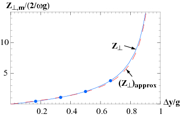
Figure 18: For the misaligned, flat pipe of aperture $2g$, the transverse impedance $Z_{\perp,m}$ as function of misalignment parameter $\Delta y/g$. Plotting symbols give ECHO results. The approximation, $(Z_{\perp,m})_{approx}$, is also shown (dashes).

Obtaining the longitudinal impedance $Z_{\parallel,long}$ for the misaligned pipe, one follows a similar procedure. In this case we find that the solution is given by

$$Z_{\parallel,long} =-\frac{1}{\pi c}\int_{0}^{\infty}\varphi_{m,B}(x,g-\Delta y)\frac{\partial\varphi_{m,A}}{\partial y}(x,g-\Delta y)\,dx\quad\quad\quad\quad[\Delta y>0]$$

$$=-\frac{2\cos\alpha}{\pi}\int_{0}^{\infty}\ln\left[\frac{\cosh x-\sin\alpha}{\cosh x+\sin 3\alpha}\right]\frac{dx}{\cosh x-\sin\alpha}\ ,$$ (54)

with $\alpha=\frac{1}{2}\pi\Delta y/g$. We solve the integral numerically. The result, for $\Delta y>0$, is plotted in Fig. 19. Note that $Z_{\parallel,long}$ is even with respect to $\Delta y$. The plotting symbols give ECHO results, and we see reasonably good agreement with our results. As a scale comparison the impedance of a round, step-out transition, from radius $g$ to radius $g+\Delta y$, $(Z_{\parallel,long})_{round}=4\ln(1+\Delta y/g)/c$, is also given in the plot (the dashes).

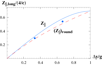
Figure 19: For the misaligned, flat pipe of aperture $2g$, the longitudinal impedance $Z_{\parallel,long}$ as function of misalignment parameter $\Delta y/g$. Plotting symbols give ECHO results. As a scale comparison the impedance of a round, step-out transition, from radius $g$ to radius $g+\Delta y$, $(Z_{\parallel})_{round}=4\ln(1+\Delta y/g)/c$, is also given (dashes).

U2. LCLS Rectangular-to-Round Transition

In the LCLS undulator region there are 33 pairs of rectangular-to-round transitions. The rectangular aperture has horizontal width $2w=10$ mm by vertical height $2g=5$ mm; the round aperture has radius $a=4$ mm. The axes of the two pipes are aligned. The transitions are abrupt. The bunch length in this region is 20 $\mu$m (rms). Thus our optical regime formulas are applicable. Note that these transitions are neither step-in nor step-out transitions. In the LCLS undulator region the longitudinal impedance is the more important one, and this is the one we calculate here. A numerical ECHO calculation has found that the longitudinal impedance of a pair of transitions (one rectangular-to-round and one round-to-rectangular transition) equals $1.21/c$ BaneZ06 .

Beginning with Eq. (11), and using Green’s first identity, we obtain

$$Z_{\parallel,long}=-\frac{1}{2\pi c}\int_{C_{G}}\varphi_{m,B}{\bf n}\cdot\nabla\varphi_{m,A}\,d\ell\ .$$ (55)

Here $S_{G}$ is the intersection of $S_{A}$ and $S_{B}$. The integration path $C_{G}$ follows the rectangular boundary at the top and bottom, and the circular boundary on the right and left (see Fig. 16). In the rectangular-to-round case [or we can say the rectangular-to-circular (rtc) case] with impedance $Z_{\parallel,rtc}$ region $A$ is the rectangular pipe, region $B$ is the circular pipe. In the circular-to-rectangular (ctr) case with impedance $Z_{\parallel,ctr}$ the regions are reversed.

The circular monopole potential is given by $\varphi_{m,c}=-\ln[(x^{2}+y^{2})/a^{2}]$; and the rectangular monopole potential, by $\varphi_{m,r}=G(x,y,0)$, with $G$ given by Eq. (44). Then we have as rectangular-to-circular impedance

$$Z_{\parallel,rtc}=-\frac{2}{\pi c}\int_{0}^{\sqrt{a^{2}-g^{2}}}\!\!\!\!\!\!\!\!\varphi_{m,c}(x,g)\frac{\partial\varphi_{m,r}}{\partial y}(x,g)\,dx\ .$$ (56)

The contribution from the circular part of the boundary is zero, since $\varphi_{m,c}$ is zero on this boundary. In the circular-to-rectangular case

$$Z_{\parallel,ctr}=-\frac{2a}{\pi c}\int_{0}^{\arctan(g/\sqrt{a^{2}-g^{2}})}\!\!\!\!\!\!\!\!\!\!\varphi_{m,r}(a\cos\theta,a\sin\theta)\frac{\partial\varphi_{m,c}}{\partial r}(a\cos\theta,a\sin\theta)\,d\theta\ ,$$ (57)

where $\partial\varphi_{m,c}/\partial r(x,y)=-2/\sqrt{x^{2}+y^{2}}$. The contribution from the rectangular part of the boundary is zero, since $\varphi_{m,r}$ is zero on this boundary. These integrals can easily be solved numerically, and the sums coming from $\varphi_{m,r}$ converge well.

To do a small parameter study, let us keep the shape of the rectangular pipe fixed, with $w=2g$, and let us vary $a$ from $g$ to $w$. In Fig. 20 we plot the results, giving the impedance of a rectangular-to-circular transition, $Z_{\parallel,rtc}$, of a circular-to-rectangular transition, $Z_{\parallel,ctr}$, and the sum of one of each type, $(Z_{\parallel})_{total}$, as functions of $a/g$. We see that each of the single transition curves goes to zero exactly where that transition becomes a step-in transition. For the actual design of the LCLS transition ($a/g=1.6$), the $rtc$ transition has 7.5 times the impedance of the $ctr$ transition. In Fig. 20 the black dot gives $(Z_{\parallel})_{total}$ as obtained by ECHO, and we see good agreement: our calculation gives $1.24/c$ and the ECHO result is $1.21/c$.

Figure 20: Longitudinal impedance for transitions of the LCLS rectangular-to-circular type, giving $Z_{\parallel,rtc}$, $Z_{\parallel,ctr}$, and their sum $(Z_{\parallel})_{total}$ as functions of circular radius $a$. The rectangle width $2w=4g$. The ECHO result for $(Z_{\parallel})_{total}$, from Ref. BaneZ06 , is given by the black dot.

VII Conclusions

We have used a method, that we derived in a companion report Stupakov07 , to find impedances in the optical regime, and applied it to various 3D beam pipe transitions that one encounters in vacuum chambers of accelerators. The method is applicable to high frequencies and transitions that are short compared to the catch-up distance. Our examples are of four types: an iris/short collimator in a beam pipe, a step-in transition, a step-out transition, and more complicated transitions. (Note that a long collimator with ends that are short transitions has an impedance that is the sum of the impedances of a step-in and a step-out transition, and is thus also included.) Most of our results are analytical, with a few given in terms of a simple one dimensional integral. We believe that all of our results are new. We have also compared (most of) our results with numerical simulations with the computer program ECHO, a finite-difference program that solves Maxwell’s equations of an ultra-relativistic bunch within metallic boundaries of 3D geometry, and the agreement is excellent. Note that our method is a much simpler way of obtaining impedances than the simulations.

We have focused on transverse impedances. For bi-symmetric (horizontal and vertical mirror symmetric) examples, a bunch moving at a small offset from the symmetry axis will excite a transverse impedance composed of both a dipole and a quadrupole component. For such problems we give both components. The iris/short-collimator-in-a-beam-pipe examples we solve include irises with small aperture that are (I1) flat, (I2) rectangular, (I3) elliptical; also included is (I4) a flat iris (not necessarily small) in a flat beam pipe. An interesting result is that the vertical impedance of an elliptical iris is independent of the horizontal axis of the ellipse.

For a step-in transition of any shape we find that all impedances (transverse and longitudinal) are zero. For a step-out transition (which in the optical regime has the same impedance as a long collimator) we give the solution for (T1) a flat step-out transition to a flat beam pipe, (T2) a rectangular step-out transition, and (T3) an elliptical step-out transition. We find, for example, that the transverse impedance of a flat, long collimator in a flat beam pipe is $\pi^{2}/8$ times the impedance of the inscribed round, long collimator in a round beam pipe. The more complicated transitions examples we solve are (U1) misaligned flat pipes and (U2) the LCLS rectangular-to-round transitions.

The method of Ref. Stupakov07 is powerful; it allows one to calculate the impedance in the optical regime of a truly large class of transitions. We have demonstrated this with a small number of relatively simple examples, compared to what is possible.

Appendix: Limiting Values of the Impedance of Elliptical Transitions

The solution for the elliptical step-out transition with axes $w$ by $g$ (horizontal by vertical), Eqs. 48, can be written as

$$Z_{\perp,d} =\frac{4(1-\beta)^{2}}{\omega g^{2}\beta}\sum_{m=1}^{\infty}\frac{2m-1}{\beta^{-(2m-1)}-1}\ ,$$

$$Z_{\perp,q} =\frac{8(1-\beta)^{2}}{\omega g^{2}\beta}\sum_{m=1}^{\infty}\frac{m}{\beta^{-2m}+1}\ ,$$ (58)

where $\beta=(w-g)/(w+g)$. We derive here the limits for $\beta=0$ (a step-out transition from a round beam pipe), $\beta=1$ (from an elliptical pipe with infinitesimal height), and $\beta=-1$ (from an elliptical pipe with infinitesimal width).

The Limit for $\beta=0$

In this limit, only the $m=1$ term contributes to $Z_{\perp,d}$ and no term contributes to $Z_{\perp,q}$. We obtain the round step-out transition results

$$Z_{\perp,d}=\frac{4}{\omega g^{2}}\ ,\quad\quad Z_{\perp,q}=0\ .$$ (59)

The Limit for $\beta=1$

Let us consider the dipole impedance first. For $\beta=1-\epsilon$, with $\epsilon$ a small positive number, the sum peaks when $2m\epsilon\approx\ln m$, i.e. for a large value of $m$. Thus the sums can be replaced by integrals, $\sum_{m}\to\int dm$. Changing variables to $x=\beta^{-(2m-1)}$, $dx=-2(\ln\beta)x\,dm$, we obtain

$$Z_{\perp,d}=\lim_{\beta\to 1}\frac{2}{\omega g^{2}}\frac{(1-\beta)^{2}}{\beta(\ln\beta)^{2}}\int_{1}^{\infty}\frac{\ln x}{(x-1)}\frac{dx}{x}\ .$$ (60)

The integral equals $\pi^{2}/6$, and

$$\lim_{\beta\to 1}\frac{(1-\beta)^{2}}{\beta(\ln\beta)^{2}}=1\ .$$ (61)

The calculation for $Z_{\perp,q}$ is similar. Our final result is the same as for the flat pipe step-out transition

$$Z_{\perp,d}=\frac{\pi^{2}}{3\omega g^{2}}\ ,\quad\quad Z_{\perp,q}=\frac{\pi^{2}}{6\omega g^{2}}\ ,\quad\quad Z_{\perp}=\frac{\pi^{2}}{2\omega g^{2}}\ .$$ (62)

The Limit for $\beta=-1$

Let $\gamma=-\beta$. Then our equations become

$$Z_{\perp,d} =\frac{4(1+\gamma)^{2}}{\omega g^{2}\gamma}\sum_{m=1}^{\infty}\frac{2m-1}{\gamma^{-(2m-1)}+1}\ ,$$

$$Z_{\perp,q} =-\frac{8(1+\gamma)^{2}}{\omega g^{2}\gamma}\sum_{m=1}^{\infty}\frac{m}{\gamma^{-2m}+1}\ .$$ (63)

To find the leading order behavior of $Z_{\perp}$ we need to go to second order in the calculation. To do this we will use the Euler-Maclaurin formula relating sums to integrals wiki

$$\sum_{m=1}^{\infty}f(m)\approx\frac{f(1)}{2}+\int_{1}^{\infty}f(x)\,dx-\frac{1}{12}f^{\prime}(1)\ ,$$ (64)

where ^′ denotes taking the derivative of a function. The formula is valid if the sum converges. The approximation is good if $\int_{1}^{\infty}|f{{}^{\prime\prime\prime}}(x)|\,dx$ is small.

Let us consider first the dipole part. We want the solution for $\gamma=1-\epsilon$, with $\epsilon$ a small, positive parameter that we, in the end, let go to zero. For the dipole part

$$f(m)=\frac{16}{\omega g^{2}}\frac{2m-1}{\gamma^{-(2m-1)}+1}\ .$$ (65)

There are three terms on the right side of Eq. 64 that we need to calculate. The first term $f(1)/2=4/(\omega g^{2})$. The integral term, done like before, is

$$\int_{1}^{\infty}f(x)\,dx=\lim_{\gamma\to 1}\frac{8}{\omega g^{2}}\frac{1}{(\ln\gamma)^{2}}\int_{1/\gamma}^{\infty}\frac{\ln x}{(x+1)}\frac{dx}{x}\ .$$ (66)

Note that for this order of calculation, in the integral on the right, the lower limit of integration is $1/\gamma$ instead of 1. This integral

$$\int_{1/\gamma}^{\infty}\frac{\ln x}{(x+1)}\frac{dx}{x}=\frac{\pi^{2}}{6}-\ln\left(\frac{1+\gamma}{\gamma}\right)\ln{\gamma}-\frac{1}{2}(\ln{\gamma})^{2}+{\rm Li}_{2}(-1/\gamma)\ ,$$ (67)

with ${\rm Li}_{2}(x)$ the polylogarithmic function of order 2. We combine this result with the terms in front of the integral in Eq. 66, expand around $\gamma=1$, and substitute $\gamma=(g+w)/(g-w)$; we find that the second, integral contribution to Eq. 64 equals

$$\frac{1}{\omega}\left[\frac{\pi^{2}}{6w^{2}}+\left(\frac{\pi^{2}}{18}-2\right)\frac{1}{g^{2}}\right]\ .$$

The third term in Eq. 64, $-f^{\prime}(1)/12=-4/(3g^{2})$. We sum all three contributions to obtain $Z_{\perp,d}$. Exactly the same technique is used for $Z_{\perp,q}$ (note, however, that the equation corresponding to Eq. 66 will have an integral with lower limit $1/\gamma^{2}$, not $1/\gamma$). We finally obtain

$$Z_{\perp,d} =\frac{1}{\omega}\left[\frac{\pi^{2}}{6w^{2}}+\left(\frac{2}{3}+\frac{\pi^{2}}{18}\right)\frac{1}{g^{2}}\right]$$

$$Z_{\perp,q} =\frac{1}{\omega}\left[-\frac{\pi^{2}}{6w^{2}}+\left(\frac{4}{3}-\frac{\pi^{2}}{18}\right)\frac{1}{g^{2}}\right]\ .$$ (68)

The leading order behavior of these impedances, in this limit, is $Z_{\perp,d}=-Z_{\perp,q}=\pi^{2}/(6\omega w^{2})$. Summing the two impedances together, we find that the total impedance equals $Z_{\perp}=2/(\omega g^{2})$. This value of total impedance is the same as we found for any small elliptical iris in a beam pipe. This result appears to agree with the numerical calculation of the original sums, which is plotted in Fig. 15.

References

- (1) K. Yokoya, in 2005 International Linear Collider Physics and Detector Workshop and Second ILC Accelerator Workshop (Snowmass, CO, 2005).
- (2) Report SLAC-R-593, 2002.
- (3) G. Stupakov, K. Bane, I. Zagorodnov, “Optical approximation in the theory of geometric impedance,” SLAC-PUB-12369, February 2007.
- (4) V. E. Balakin and A. V. Novokhatski, in Proceedings of the 12th International Conference on High-Energy Accelerators, edited by F. T. Cole and R. Donaldson (Fermilab, Batavia, IL, 1983), p. 117.
- (5) S. A. Heifets and S. A. Kheifets, Rev. Modern Phys. 63, 631 (1991).
- (6) E. Gianfelice and L. Palumbo, IEEE Trans. Nucl. Sci. 37, 1081 (1990).
- (7) F. Zimmermann, et al, in Proceedings of the European Particle Accelerator Conference, Sitges, 1996 (1996), pp. 504–506.
- (8) I. Zagorodnov and K. L. F. Bane, in Proceedings of the European Particle Accelerator Conference, Edinburgh, 2006 (2006), pp. 2859–2861.
- (9) K. L. F. Bane and I. Zagorodnov, in Proceedings of the European Particle Accelerator Conference, Edinburgh, 2006 (2006), pp. 2952–2954.
- (10) I. Zagorodnov and T. Weiland, Phys. Rev. ST-AB 8, 042001 (2005).
- (11) W. K. H. Panofsky and W. Wenzel, Rev. Sci. Instr. 27, 967 (1956).
- (12) J. D. Jackson, Classical Electrodynamics, 3rd Ed., (J. Wiley & Sons, New York, 2001).
- (13) P. Morse and H. Feshbach, Methods of Theoretical Physics, Part II, (McGraw-Hill, New York, 1953), p. 1240.
- (14) R. Gluckstern, J. Van Zeijts, B. Zotter, Phys. Rev. E 47, No. 1, 656 (1993).
- (15) See e.g. C. M. Bender and S. A. Orszag, Advanced Mathematical Methods for Scientists and Engineers I: Asymptotic Methods and Pertubation Theory, (Springer, New York, 1999), p. 305.