On the occurrence of Balmer spectra in expanding microplasmas from laser irradiated liquid hydrogen

Abstract

Balmer spectra are investigated which are obtained from hydrogen droplets irradiated by ultra-short intense laser pulses. A unified quantum statistical description of bremsstrahlung, the Stark broadening and the van der Waals profile of hydrogen spectral lines is used, which allows to include many-particle effects. Analyzing the line profiles, a low ionization degree of a dense plasma is inferred, where the main contribution to the spectral line shape originates from the interaction with the neutral components. Effective temperatures and densities of the radiating microplasma are deduced. A dynamical description is given within plasma hydrodynamics, explaining the formation of excited atomic states in the expanding system and the occurrence of the observed Balmer lines only below a critical density.

I Introduction

Spectroscopy is one of the most powerful methods in plasma diagnostics. In particular, the analysis of the shape of spectral lines allows to determine the properties of the plasma such as temperature, density, and composition. For dense, strongly coupled plasmas, optical spectra have been investigated to infer the parameter values not only of laboratory, but also of astrophysical plasmas, see, e.g. Refs. Flohr and Piel (1993); Godbert et al. (1994); Malyshev and Donnelly (1999); Tadokoro et al. (1998) and Refs. Soria et al. (2000); Benz (2002); Rybicki and Lightman (1975), respectively.

The shape of spectral lines is determined by different processes. Besides the natural line width given by the finite lifetime of excited states, Doppler broadening is related to the thermal motion of the emitters. The influence of the surrounding medium becomes more important at increasing density and leads to pressure broadening. A large effect is caused by charged particles in the plasma. This Stark broadening is determined by the distribution of ions as sources of the microfield, whereas the contribution of the electrons is usually treated in impact approximation Baranger (1962); Griem and Kolb (1958). The Weisskopf radius can be used to distinguish between weak and strong collisions. However, also the neutral components in the surrounding medium contribute to line profile, i.e. as van der Waals broadening.

A systematic approach to the shape of spectral lines in dense plasmas has been worked out on the basis of perturbation theory Sobelmann et al. (1981), and many-particle effects have been incorporated. Griem Griem (1964) gives a review of different classical and semiclassical methods as well as their application to line shapes in different plasmas. The unified theory Smith et al. (1969); Voslamber (1969) was developed to describe the center as well as the wings of the lines. A quantum statistical approach based on the many-particle Green functions method was presented by Günter Günter et al. (1991); Günter (1995) and has been developed systematically for charged perturbers. Special attention was payed to show the equivalence between this rigorous approach and the aforementioned classical and semiclassical concepts in the appropriate limits. The quantum statistical approach has been applied to a broad range of systems, e.g. hydrogen plasmas Röpke et al. (1981); Hitzschke et al. (1986); Günter et al. (1991); Könnies and Günter (1994), helium plasmas Milosavljević and Djeniźe (2003); Omar et al. (2006) and plasmas of other elements containing H or He like ions. In most cases, a hot and dense plasma with a large fraction of free electrons was considered. In such systems, the main contribution to the shift and width of a given spectral line, besides the natural line width and Doppler broadening, comes from the ionic microfield, caused by ions surrounding the radiating atom or ion, collisions with free electrons, and interaction with collective excitations in the plasma (plasmons). Theoretical results are in very good agreement with experiments carried out, e.g. by Wilhein Wilhein et al. (1998); Sorge et al. (2000).

In weakly ionized plasmas, the influence of neutral perturbers becomes dominant. Van der Waals broadening has been investigated within second order perturbation theory. Based on the derivation of the van der Waals potential between two hydrogen atoms in their ground state as given by London Eisenschitz and London (1930), a red shift of the spectral line follows as was shown by Margenau Margenau (1935). A review of van der Waals broadening is given by Traving Traving (1995). Line broadening due to van der Waals interaction has been investigated in detail, e.g. by Walkup et al. Walkup et al. (1984).

We show how to extend the quantum statistical approach, elaborated for the influence of charged particles on the line profile, to include also the interaction with neutral perturbers. In this way, the extension of the van der Waals broadening by accounting for many-particle effects such as dynamical screening or strong collisions is possible. A unified description of the influence of the perturbing partially ionized plasma on the line profile of a radiating atom can be performed, treating charged particles and neutrals within the same formalism.

The theory will be compared to optical spectra obtained from hydrogen microdroplets exposed to strong femtosecond laser pulses. So far, most of the experimental and theoretical work has concentrated on nanosized clusters Ditmire et al. (1996); Döppner et al. (2005); Kim et al. (2003). Studies on the light emission from these systems have focused on x–rays and EUV–radiation Fan et al. (2000); Schnürer et al. (2001); Düsterer et al. (2001), motivated, e.g. by the search for novel light sources. Hydrogen as a target material has attracted considerable attention since nuclear fusion has been demonstrated as a result of Coulomb explosion of dense deuterium clusters Madison et al. (2004). Various efforts to produce micrometer sized hydrogen targets are reported, cf. e.g. Ref. Nordhage et al. (2005). Other studies on such large systems include, e.g. the measurement of x–ray emission from Kr clusters Hansen et al. (2005) and from methanol microdroplets Anand et al. (2005, 2006). An expanding microplasma can be produced with interesting parameter values. In particular, strongly coupled plasmas are obtained, where density and temperature are time-dependant. Time resolved experimental techniques have been demonstrated to measure transient plasma properties like the evolution of the plasma density Zweiback et al. (2000a); Liu et al. (2006).

In the experiment on $\mu$m sized droplets reported here, lines of the hydrogen Balmer series are observed as distinctive features in the optical emission spectrum. The present paper will give a first interpretation of the recorded line shapes. The analysis of the line profiles shows that van der Waals broadening due to neutral perturbers is the predominant contribution. Values for the effective plasma parameters are deduced to interprete the observed line profiles, which differ for the different lines. However, an equilibrium picture cannot give an agreeable description of the measured Balmer spectra. A consistent dynamical picture of the expanding microplasma will be given by use of hydrodynamic simulations. This enables us to interpret the observed spectra if considering the time stages where excited atomic states can exist.

The work is organized as follows: In the second section we will briefly outline the method of thermodynamic Green functions with emphasis on its application to the calculation of spectral line shapes. The method will be applied to the case of a weakly ionized plasma, where the interaction among atoms is governed by the dipole-dipole term. The Margenau result appears in the case of ground state perturbers. In the third section, our results will be compared to the Balmer spectra obtained from laser produced hydrogen microplasmas. Parameter values for the effective temperature and density are inferred. In the fourth section, a hydrodynamical description of the expanding droplet after laser excitation is given.

II Many-body theory of line shapes and van der Waals broadening

II.1 Quantum statistical approach to spectral line shapes

A quantum statistical approach to the optical spectra of dense, strongly coupled systems can be given within linear response theory. Emission and absorption of radiation is related to the transverse dielectric function $\epsilon_{\rm tr}(\vec{k},\omega)$. In the optical region, the wavelength is large compared with atomic distances so that the long-wavelength limit $k\to 0$ can be considered. For the absorption coefficient we find

$$\alpha(\omega)=\frac{\omega}{cn(\omega)}\mathrm{Im}\,\epsilon(0,\omega)~{},$$ (1)

$n(\omega)$ is the refraction index, $c$ is the velocity of light in vacuum. For $k\to 0$ the transverse and longitudinal dielectric function $\epsilon(0,\omega)$ become identical. We consider in the following the longitudinal one.

The dielectric function for a charged particle system can be evaluated in a rigorous way using quantum statistical methods. According to $\epsilon(\vec{k},\omega)=1-(1/\epsilon_{0}k^{2})\Pi(\vec{k},\omega)$, it is linked to the polarization function $\Pi(\vec{k},\omega)$, for which a systematic perturbation expansion can be given. A Green function approach to the polarization function is outlined in App. A. Using Feynman diagrams and partial summations, appropriate approximations can be found which account for different microscopic processes contributing to the behavior of the charged particle system. In particular, for partially ionized plasmas, a cluster decomposition $\Pi(\vec{k},\omega)=\Pi_{1}(\vec{k},\omega)+\Pi_{2}(\vec{k},\omega)+\ldots$ can be performed to give the contribution of free carriers as well as of bound states in a systematic way Röpke and Der (1979).

$\Pi_{1}(\vec{k},\omega)$ collects the single-particle contribution. In lowest order, neglecting collisions with other particles, the well-known RPA polarization function

$$\Pi_{1}^{(0)}(\vec{k},\omega)=\Pi^{\mathrm{RPA}}(\vec{k},\omega)=\sum_{c,\vec{p}}e_{c}^{2}{f_{c}(\vec{p})-f_{c}(\vec{p}-\vec{k})\over E^{c}_{p}-E^{c}_{\vec{p}-\vec{k}}-\hbar\omega-i\eta}$$ (2)

is obtained. Here, $f_{c}(\vec{p})=[\exp\{(E^{c}_{p}-\mu_{c})/k_{B}T\}+1]^{-1}$ is the Fermi distribution function of particles of species $c$ (including spin) with charge $e_{c}$ and mass $m_{c}$, $E^{c}_{p}=\hbar^{2}p^{2}/2m_{c}$ is the single-particle kinetic energy, and $\mu_{c}$ the chemical potential. Within this lowest order approximation, single-particle excitations as well as collective plasmon modes are described. The limit $\eta\to 0^{+}$ has to be performed after the summation over momenta.

The RPA contribution $\Pi_{1}^{(0)}(\vec{k},\omega)$ is improved if interactions with other particles beyond mean field are included, see App. A. Medium effects, such as collisions, dynamical screening and exchange, enter the polarization function via the single-particle self-energies and the vertex function. The vertex function describes the in-medium coupling of particles to the radiation field. It has to be taken in the same approximation as the self-energy as dictated by consistency constraints, i.e. Ward identities Mahan (1981). Going beyond the mean-field (Hartree-Fock) approximation, collisions can be considered in lowest order Born approximation. Higher orders lead to dynamical screening and t-matrix expressions for strong collisions. This way, the continuum of optical spectra is described, in particular inverse bremsstrahlung Wierling et al. (2001). However, line spectra are missing in $\Pi_{1}(\vec{k},\omega)$.

The next term in the cluster decomposition is $\Pi_{2}(\vec{k},\omega)$. It is given by the convolution of two atomic (two-particle) propagators and describes also transitions between bound states, i.e. the line spectrum Röpke and Der (1979). In the lowest order, any interaction with further particles are neglected. Similar to $\Pi^{(0)}_{1}(\vec{k},\omega)$ given above, replacing single-particle propagators by atomic propagators one obtains

$$\Pi^{(0)}_{2}(\vec{k},\omega)=4\sum_{\alpha_{1}\alpha_{2},\vec{P}}\left|M_{\alpha_{1}\alpha_{2}}^{(0)}(\vec{k})\right|^{2}{g(E^{(0)}_{\alpha_{1}\vec{P}})-g(E^{(0)}_{\alpha_{2}\vec{P}-\vec{k}})\over E^{(0)}_{\alpha_{1}\vec{P}}-E^{(0)}_{\alpha_{2}\vec{P}-\vec{k}}-\hbar\omega-i\eta}~{}.$$ (3)

The factor 4 accounts for spin degeneration, $g(E^{(0)}_{\alpha\vec{P}})=[\exp\,\{(E^{(0)}_{\alpha\vec{P}}-\mu_{\mathrm{i}}-\mu_{\mathrm{e}})/k_{B}T\}-1]^{-1}$ is the Bose distribution function of electron-ion bound states at $E^{(0)}_{\alpha P}=-Z^{2}\,\mathrm{Ry}/n^{2}+\hbar^{2}P^{2}/2M$, with $\alpha=\{n,l,m,m_{s}\}$ denoting the internal quantum numbers, $\hbar\vec{P}$ the center of mass momentum, and $M=m_{\mathrm{i}}+m_{\mathrm{e}}$. The unperturbed matrix elements $M_{\alpha_{1}\alpha_{2}}^{(0)}(\vec{k})$ are given by

$$M_{\alpha_{1}\alpha_{2}}^{(0)}(\vec{k}) =e\sum_{p}\psi_{\alpha_{1}}^{*}(\vec{p})\left[\psi_{\alpha_{2}}(\vec{p}-\frac{m_{\mathrm{e}}}{M}\vec{k})-\psi_{\alpha_{2}}(\vec{p}+\frac{m_{\mathrm{i}}}{M}\vec{k})\right]$$ (4)

$$\simeq e\left[\delta_{\alpha_{1}\alpha_{2}}-\int\!\mathrm{d}^{3}\vec{r}\,\psi_{\alpha_{1}}^{*}(\vec{r})\,\mathrm{e}^{i\vec{k}\cdot\vec{r}}\,\psi_{\alpha_{2}}(\vec{r})\right]~{}.$$ (5)

$\psi_{\alpha}(\vec{p})=\langle\,\vec{p}\,|\,\alpha\,\rangle$ and $\psi_{\alpha}(\vec{r})=\langle\,\vec{r}\,|\,\alpha\,\rangle$ are atomic wave-functions in relative momentum representation and coordinate representation, respectively. Eq. (5) results for $m_{\mathrm{e}}/m_{\mathrm{i}}\to 0$. In contrast to a simple chemical picture where a mixture of free charge carriers and atoms is considered, scattering states are included, and double counting of diagrams has to be avoided. In this approximation, one obtains the unperturbed line-spectrum of isolated atoms including the Doppler profile due to thermal motion.

As before, medium effects are described by taking the self-energy of the constituents and the vertex into account, which now are given on the two-particle level, see App. A. In the simplest approximation, the dynamically screened interaction can be considered similar to the $GW$ approximation for the single-particle propagator C. Fortmann, G. Röpke, and A. Wierling, physics/0610262, accepted for publication in Contrib. Plasma Phys. . This dynamically screened interaction contains the polarization function, which once more can be decomposed into the contribution of single-particle states, two-particle states and higher cluster states. In this way, we obtain the dynamically screened Born approximation for collisions with free particles or composed clusters of the partially ionized plasma.

In the case of dense and strongly ionized systems, the main contribution to the self-energy comes from the interaction of the radiating atom with charged particles, i.e. electrons and ions. The influence of free particles is given by the RPA-polarization function, i.e. the first term in the cluster decomposition. This interaction can be inserted into the self-energy, but the vertex-function has to be taken in the same approximation. Reducing the screened interaction to its one-loop approximation, which amounts to the second Born approximation with respect to the statically screened Coulomb potential, the so-called impact approximation is obtained. Systematic improvements by taking higher order contributions into account lead to the dynamical screening of the Coulomb potential in the case of weak collisions and the t-matrix approach in the case of strong collisions. In particular, the contribution of collisions with electrons to the line profile in dense plasmas is treated this way, for a review see Günter Günter (1995).

The following expression for the line-profile $\mathcal{L}(\Delta\omega)$ as a function of the frequency displacement $\Delta\omega=\omega-(E_{i}^{0}-E_{f}^{0})/\hbar$ is obtained Günter (1995),

$$\mathcal{L}(\Delta\omega)=\sum_{ii^{\prime}ff^{\prime}}M_{if}^{(0)}(\vec{k})\left[M_{i^{\prime}f^{\prime}}^{(0)}(\vec{k})\right]^{*}\frac{\mathrm{e}^{-\beta\hbar(\omega_{if}+\Delta\omega)}\left(\omega_{if}+\Delta\omega\right)^{4}}{8\pi^{3}c^{3}}\int\frac{\mathrm{d}^{3}P}{(2\pi)^{3}}\,\mathrm{e}^{-\beta\frac{\hbar^{2}P^{2}}{2M}}\,\int_{0}^{\infty}\mathrm{d}\bar{\beta}\,W_{\rho}(\bar{\beta})\\ \times\langle\left.\,i\,\right|\langle\left.\,f\,\right|\left[\hbar\Delta\omega-\frac{\hbar^{2}\vec{P}\cdot\vec{k}}{M}-\frac{\hbar^{2}k^{2}}{2M}-\mathrm{Re}\,\left\{\Sigma_{i}(\Delta\omega,\bar{\beta})-\Sigma_{f}\right\}+i\mathrm{Im}\,\left\{\Sigma_{i}(\Delta\omega,\bar{\beta})+\Sigma_{f}\right\}+i\Gamma^{v}\right]^{-1}\left|\,f^{\prime}\,\right.\rangle\left|\,i^{\prime}\,\right.\rangle~{}.$$ (6)

Here, $\Sigma_{i},\Sigma_{f}$ denote the electronic contribution to the self-energy of the initial or final state, respectively, $\Gamma^{v}$ the vertex contribution. Improvements of the Born approximation by accounting for dynamical screening and strong collisions, have extensively been discussed in the literature Griem (1964).

Due to their large masses, ions are much slower than electrons. In the adiabatic limit, the ions may be considered as a static distribution of charged particles during the process of emission. Considering different ionic configurations in the plasma, the distribution $W_{\rho}(\bar{\beta})$ of the so-called microfield $\bar{\beta}=E/E_{\rm Holtsmark}$, $E_{\rm Holtsmark}=(4n_{\mathrm{ion}}/15)^{2/3}Ze/(2\epsilon_{0})$, ($n_{\mathrm{ion}}$ is the density of ions with charge Z in the system) is introduced, and the averaging leads to the Stark profile as given in Eq. (6). Also in the case of ionic contributions, the systematic many-particle treatment leads to further improvements such as the dynamic microfield.

In the next step, one has to take into account the interaction between the radiator and neutral particles (atoms), as well. This can be performed along the same lines as for the interaction with charged particles, discussed before. The bound state contribution is considered in the cluster decomposition of the polarization function, expanding the dynamically screened interaction which enters the self-energy, see App. A. In particular we will consider the two-particle self-energy describing the influence of the medium on the radiator, where the bound state component is taken into account in lowest approximation. We consider the second order Born approximation with respect to the unscreened Coulomb potential to describe the interaction between neutrals. The detailed calculation is given in the next section.

Again, improvements can be obtained systematically. By calculating the dynamically screened interaction with the polarization function up to the second term in the cluster decomposition, the interaction with free and bound particles as well as with collective excitations could be included in a consistent way. Strong collisions can be described via the four-particle t-matrix. In addition to the self-energy term, also the vertex is modified if bound states are included.

II.2 Evaluation of atom-atom interaction in Born approximation

The calculation of the interaction $V_{\alpha_{1}\alpha_{2}}(R)$ between two atoms at distance $R$ in state $\left|\alpha_{1}\!\right.\rangle$ and $\left|\alpha_{2}\!\right.\rangle$ is carried out in App. B. We obtain

$$V_{\alpha_{1}\alpha_{2}}(R) = {e^{4}\over(4\pi\epsilon_{0})^{2}}\sum_{\alpha_{3}\alpha_{4}}\frac{1}{E^{(0)}_{\alpha_{1}}+E^{(0)}_{\alpha_{2}}-E^{(0)}_{\alpha_{3}}-E^{(0)}_{\alpha_{4}}}$$ (7)

$$\times\left|\sum_{\vec{r}_{1}\vec{r}_{2}}\psi_{\alpha_{1}}^{*}(\vec{r}_{1})\psi_{\alpha_{3}}(\vec{r}_{1})\left[\frac{1}{R}-\frac{1}{|\vec{R}-\vec{r}_{1}|}-\frac{1}{|\vec{R}+\vec{r}_{2}|}+\frac{1}{|\vec{R}-\vec{r}_{1}+\vec{r}_{2}|}\right]\psi_{\alpha_{2}}^{*}(\vec{r}_{2})\psi_{\alpha_{4}}(\vec{r}_{2})\right|^{2}~{}.$$

Here, $\alpha_{3},\alpha_{4}$ denote quantum numbers of the intermediate states. Only elastic processes are considered where the internal quantum numbers for the initial state and the final state are identical. Due to the ion’s heavy mass, we neglect the contribution of kinetic energy in the intermediate propagator in comparison with the excitation energies. Besides $R$ which is the distance between the nuclei of the interacting atoms, $\vec{r}_{1}$ and $\vec{r}_{2}$ are vectors of position of the two electrons of atom 1 and atom 2, respectively.

This result (7) coincides with results from second order perturbation theory. At large distances $R/a_{B}\gg 1$ we can perform the dipole approximation using $|\vec{R}-\vec{r}|^{-1}\approx 1/R^{2}\left[R-(R^{2}+r^{2}-2\vec{R}\cdot\vec{r})/2R+3(R^{2}+r^{2}-2\vec{R}\cdot\vec{r})^{2}/8R^{2}\right]$ for $R\gg r$. We obtain the van der Waals potential,

$$V^{\rm vdW}_{\alpha_{1}\alpha_{2}}(R) = \frac{e^{4}}{(4\pi\epsilon_{0})^{2}R^{6}}\sum_{\alpha_{1}\alpha_{2}}\frac{1}{E^{(0)}_{\alpha_{1}}+E^{(0)}_{\alpha_{2}}-E^{(0)}_{\alpha_{3}}-E^{(0)}_{\alpha_{4}}}$$ (8)

$$\times\left|\sum_{\vec{r}_{1}\vec{r}_{2}}\psi_{\alpha_{1}}^{*}(\vec{r}_{1})\psi_{\alpha_{3}}(\vec{r}_{1})\left[\vec{r}_{1}\cdot\vec{r}_{2}-3\frac{\left(\vec{r}_{1}\cdot\vec{R}\right)\;\left(\vec{r}_{2}\cdot\vec{R}\right)}{R^{2}}\right]\psi_{\alpha_{2}}^{*}(\vec{r}_{2})\psi_{\alpha_{4}}(\vec{r}_{2})\right|^{2}~{}.$$

For hydrogen-like atoms, the sum in Eq. (8) has been performed by Eisenschitz and London Eisenschitz and London (1930). Their result for the interatomic potential between two hydrogen atoms in ground state ($\alpha_{1}=\alpha_{2}=1s$) is given by

$$V^{\mathrm{vdW}}_{1s,1s}(R)=-\frac{C_{6}}{R^{6}}~{}.$$ (9)

The constant $C_{6}$ was calculated as $C_{6}=12.94\,\mathrm{Ry}\,\,a_{\mathrm{B}}^{6}$, where $\,\mathrm{Ry}=13.6\,\mathrm{eV}$ is the Rydberg energy and $a_{\mathrm{B}}=0.53$ Å is the Bohr radius.

For the interaction between a radiator in an excited state $\alpha=n,l$ and a perturber in ground state, $\alpha=1s$, the following expression for the interaction strength $C_{6}(\alpha,1s)$, can be derived, as shown in App. C,

$$C_{6}(\alpha,1s)=4\frac{n^{2}}{1+1/n^{2}}\left[5n^{2}+1-3l(l+1)\right]~{}.$$ (10)

Note that there is no exchange contribution in Eq. (7), since the distance $R$ is assumed to be large compared with the Bohr radius. At shorter distances, the higher order terms as well as exchange terms have to be taken into account which will diminuish the van der Waals behavior at small distances and possibly, in the case of electrons in the triplet state, result in a repulsion due to the exchange contribution.

II.3 Van der Waals profiles

Within a general approach, the contribution of the dense medium to the spectral line shape is given by the self-energy and vertex contribution. The first order of the interaction gives the Hartree-Fock mean field, in second order the impact approximation is obtained where collisions are described in Born approximation.

Within this concept, the van der Waals contribution to the self-energy is

$$\Sigma_{\alpha_{1}}^{\rm vdW}=\sum_{\alpha_{2},P}g(E^{(0)}_{\alpha_{2}\vec{P}})V_{\alpha_{1}\alpha_{2}}^{\rm vdW}(q=0)~{},$$ (11)

which in coordinate space reads

$$\Sigma_{\alpha_{1}}^{\rm vdW}=\sum_{\alpha_{2}}n_{\alpha_{2}}\int d^{3}R\,\,V_{\alpha_{1}\alpha_{2}}^{\rm vdW}(R)~{}.$$ (12)

Here, $n_{\alpha_{2}}$ is the density of pertubing atoms in state $\alpha_{2}$. In the following, we consider the perturbing atoms in their ground state $\alpha_{2}\equiv 0$ not and only the radiator in an excited state $\alpha=nl,\,n>1$.

As already discussed in connection with the ionic contribution to the spectral line shapes, because of their large masses the atomic motion is slow, and we can apply the microfield concept of strong interaction with a given field distribution. The intensity distribution of a given spectral line, due interaction between the radiator in initial and final states $\left|i\!\right.\rangle$ and $\left|\,f\,\right.\rangle$, respectively and the perturber in its ground state $\left|0\!\right.\rangle$ is obtained by performing an averaging procedure over the distribution of perturbing atoms,

$$I_{if}(\Delta\omega)=\int\mathrm{d}^{3}\vec{r}_{1}\int\mathrm{d}^{3}\vec{r}_{2}\ldots\int\mathrm{d}\vec{r}_{N}P_{N}(\vec{r}_{1},\vec{r}_{2},\ldots,\vec{r}_{N})\,\delta\left(\sum_{j=1}^{N}V_{i0}(r_{j})-V_{f0}(r_{j})-\hbar\Delta\omega\right)~{}.$$ (13)

Here, $P_{N}(\vec{r}_{1},\ldots\vec{r}_{N})$ is the probability density for having atom 1 in the volume element $\mathrm{d}^{3}\vec{r}_{1}$ at $\vec{r}_{1}$, atom 2 in the volume element $\mathrm{d}^{3}\vec{r}_{2}$ at $\vec{r}_{2}$, etc. The evaluation of the sum (13) in the case of statistically independent atoms, i.e. $P_{N}(\vec{r}_{1},\ldots\vec{r}_{N})=1/V^{N}$, is shown in App. D.

The result for the dipole limit of the interaction Eq. (9) is Margenau (1935),

$$I^{\rm vdW}_{if}(\Delta\omega)=\Lambda_{if}\left[-\Delta\omega\right]^{-3/2}\mathrm{e}^{\pi\Lambda_{if}^{2}/\Delta\omega}~{},$$ (14)

with $\Lambda_{if}=(2\pi/3)\,(C_{6}(i,0)-C_{6}(f,0))^{1/2}n_{\mathrm{atom}}$. This is known as the Margenau profile. Note that $\Delta\omega$ is to be taken at negative values, i.e. the van der Waals interaction shifts the spectral line to smaller energies (red shift). The maximum of the intensity distribution (14) is located at

$$\Delta\omega_{\mathrm{max}}=-\left(\frac{2\pi}{3}\right)^{3}C_{6}\,\left(n_{\mathrm{atom}}\,\,a_{\mathrm{B}}^{3}\right)^{2}\,\,\mathrm{Ry}/\hbar~{},$$ (15)

with $C_{6}=C_{6}(i,0)-C_{6}(f,0)$ and $n_{\mathrm{atom}}$ the number density of (ground state) hydrogen atoms in the system. The full width of half maximum (FWHM) of the line is found as $\gamma=2.78\,\Delta\omega_{\mathrm{max}}$, see also Refs. Margenau (1935); Lochte-Holtgreven (1995). The Margenau profile Eq. (8) will be used in order to analyse the hydrogen Balmer spectra obtained from laser produced microplasmas. These experiments will be described in the following section.

III Experiments with laser-irradiated hydrogen droplets

III.1 Experimental setup

Hydrogen droplets are produced by expansion of pre-cooled H₂ gas at temperatures between 17 and 22 K through a 20 $\mu$m orifice into a vacuum chamber using a backing pressure of about 8 bar. At these source conditions, H₂ droplets of about $10\,\mu$m in diameter are emitted from the nozzle at a density of $n_{\mathrm{liq}}=4.2\cdot 10^{22}\,\mathrm{cm}^{-3}$. Roughly 10 mm behind the nozzle the droplets are irradiated by intense IR laser pulses generated by a Ti-Sapphire laser system with a wavelength of $\lambda_{0}=810\,\mathrm{nm}$ and a pulse energy of $E_{\mathrm{pulse}}=2.5\,\mathrm{mJ}$. The beam is focussed to a spot with a beam waist of $40\,\mu\mathrm{m}$. The pulse width $\tau$ is tuned in the range of $\tau=50-1000\,\mathrm{fs}$, corresponding to laser peak intensities between $7.0\times 10^{15}\,\mathrm{W}\,\mathrm{cm}^{-2}$ and $3.5\times 10^{14}\,\mathrm{W}\,\mathrm{cm}^{-2}$. When the droplets are exposed to the strong laser field, optical emission from the hydrogen microplasmas is observed.

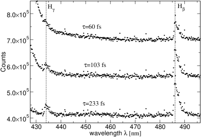
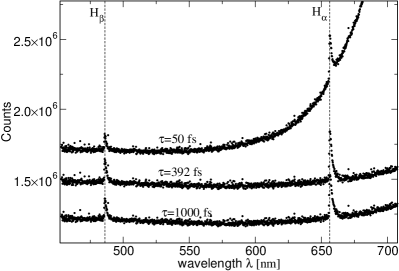
Figure 1: Representative emission spectra from laser-excited hydrogen microplasma in two spectral windows for various pulse widths $\tau$. The spectra are shifted by $1.5\cdot 10^{5}$ counts (a) and $2.5\cdot 10^{5}$ counts (b) with respect to each other. H Balmer spectral lines H${}_{\alpha},656.3\,\mathrm{nm}$, H${}_{\beta},486.1\,\mathrm{nm}$ and H${}_{\gamma},434.1\,\mathrm{nm}$ are given. The large enhancement at long wavelengths ($\lambda>660\,\mathrm{nm}$) is due to Rayleigh scattering of the laser light. 90000 shots are integrated at 1 kHz repetition rate.

The light is analyzed by a 0.34 m grating spectrometer (200 lines/mm) and monitored with a CCD camera, providing a spectral dispersion of 0.185 nm per pixel. The entrance slit width was optimized for a high signal when integrating 90000 shots at 1 kHz repetition rate. The resulting spectral resolution of the spectrometer is $\Delta\lambda\simeq 1\,\mathrm{nm}$. Two regions of the visible spectral range are analyzed in more detail, i.e. (a) $430\ldots 500$ nm, and (b) $450\ldots 700$ nm. Fig. 1 shows representative emission spectra from the laser excited hydrogen microplasmas. Elastic Rayleigh scattering of the incident radiation produces large enhancement of the measured spectra towards the excitation wavelength $\lambda_{0}$. On top of the background signal, H-Balmer spectral lines are clearly identified, i.e. H_α at $\lambda=656.3\,\mathrm{nm}$, H_β at $\lambda=486.1\,\mathrm{nm}$, and H_γ at $\lambda=434.1\,\mathrm{nm}$.

III.2 Analysis of the spectra

III.2.1 Effective Temperatures

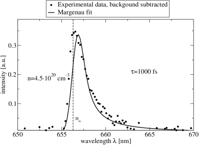
Figure 2: Comparison of experimental line profiles (dots) of H_α and H_β from the $\tau=1000\,\mathrm{fs}$ data to Margenau theory Eq. (14), taking into account the limited detector resolution $\Delta\lambda\simeq 1\,\mathrm{nm}$. For H_α, good agreement between theory and experiment was obtained setting $n^{(\alpha)}_{\mathrm{atom}}=4.5\cdot 10^{20}\,\mathrm{cm}^{-3}$. For H_β, the best fit was obtained with $n^{(\beta)}_{\mathrm{atom}}=1.8\cdot 10^{20}\,\mathrm{cm}^{-3}$.

In order to quantitatively analyze the Balmer line signals, one has to subtract the background signal. Therefore, the neighbouring spectral ranges of each line, i.e. 640..655 nm and 670..685 nm for the H_α line, 460..467 nm and 472..480 nm for H_β as well as 430..433 nm and 438..445 nm for H_γ are fitted by an exponential function, which is then subtracted from the data set. As an example, Figs. 2 (a) and (b) show the background subtracted spectra for a pulse width of $\tau=1000$ fs (dots). The solid curves are the Margenau profiles fitted to the data; they will be discussed in more detail in Sec. III.2.2.

By comparing integrated intensities from different spectral lines, one can determine the effective temperature in the system. Given the ratio of wavelength-integrated intensities $I_{1}/I_{2}$ of two spectral lines of the same atomic species and the same ionization stage at central wavelengths $\lambda_{1}$ and $\lambda_{2}$, and assuming again local thermal equilibrium, the effective temperature is Lochte-Holtgreven (1995)

$$T^{\mathrm{eff}}_{12}=\frac{E_{1}-E_{2}}{k_{\mathrm{B}}\,\ln\left[\frac{A_{1}\,g_{1}\,\lambda_{2}}{A_{2}\,g_{2}\,\lambda_{1}}\frac{I_{2}}{I_{1}}\right]}~{}.$$ (16)

$A_{1}$, $A_{2}$ are the angular momentum averaged Einstein coefficients for the transition between levels corresponding to the spectral line 1 and 2, respectively and $g_{1}$ and $g_{2}$ are the degeneracy factors of the excited level (principal quantum number $n_{i}^{\mathrm{ex}}$) of each transition, i.e. $g_{i}=2(n^{\mathrm{ex}}_{i})^{2}$. $E_{1}$ and $E_{2}$ are the energies of the excited level for each transition. Tab. 1 lists effective temperatures for each pulse width. As can be seen, $T^{\mathrm{eff}}_{12}$ is dependent on $\tau$. One obtains different results from the two ratios $I(\textrm{H}_{\alpha})/I(\mathrm{H}_{\beta})$ and $I(\textrm{H}_{\beta})/I(\mathrm{H}_{\gamma})$. For small $\tau$, $T^{\mathrm{eff}}_{\mathrm{\alpha\beta}}$ rises with increasing $\tau$. At $\tau\simeq 400\,\mathrm{fs}$, $T^{\mathrm{eff}}_{\alpha\beta}$ saturates near $1\,\mathrm{eV}$. On the other hand, $T^{\mathrm{eff}}_{\beta\gamma}$ gives values around $0.5\,\mathrm{eV}$.

Table 1: Effective line temperatures according to Eq. (16) versus pulse length. The first set of figures was obtained from the short wavelength spectrum, shown in Fig. 1(a), the second set results from the data shown in Fig. 1(b).

$\tau[fs]$	60	103	233	$\tau[fs]$	50	109	170	264	392	695	1000
$T^{\mathrm{eff}}_{\mathrm{\beta\gamma}}$ [eV]	0.49	0.56	0.41	$T^{\mathrm{eff}}_{\mathrm{\alpha\beta}}$ [eV]	0.57	0.62	0.81	0.97	0.99	1.00	1.04

These effective temperatures have to be analyzed within a microscopic description of the expanding plasma source. Self-absorption should be considered so that the intensities occurring in Eq. (16) are modified when propagating through the microplasma. Furthermore, different values $T^{\mathrm{eff}}_{12}$ from the intensities of H_α, H_β and H_γ indicates that the system is in a generic non-equilibrium state, which cannot be described by a single temperature. Despite the measured spectra are time integrated, we have to assume a dynamic evolution of the plasma parameters temperature and density over the course of the expansion of the excited hydrogen droplets. Within a hydrodynamical description given below in Sec. IV.1, local thermal equilibrium with plasma parameters depending on space and time are introduced.

During the expansion process, radiation can only be produced if the upper level of the transition in question is existent in the system so that it can be occupied. From simple geometric and energetic arguments it is clear, that $n=3,4,5$ levels are not present in hydrogen at liquid densities. This point will be discussed in more detail in Sec. IV.2.

The continuum background stems from free-bound and free-free (bremsstrahlung) transitions. The spectral behavior can also be used to estimate effective temperatures which should be analyzed within a dynamical expansion model. Since more experimental work is necessary to separate the continuum background radiation, we will consider only the line spectra in this work.

III.2.2 Spectral line shapes

To analyze the line profiles, one first has to consider the effect of the broadening due to the finite resolution of the experimental setup. The true line profile is obtained after deconvolution with the detector function. In a separate experiment the spectral resolution was measured as $\Delta\lambda\simeq 1\,\mathrm{nm}$ . This is consistent with the steep increase of intensity on the blue wing of the unperturbed spectral line.

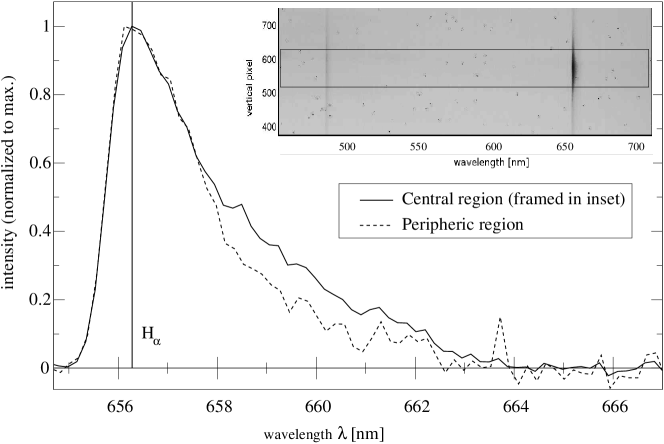
Figure 3: Normalized spectra near the $\mathrm{H}_{\alpha}$-line for $\tau=1000$ fs pulse length. The raw data (cf. inset) have been summed over different vertical ranges. The solid line marks the central region of the laser focus (framed part in the inset), the dashed curve corresponds to the data from the peripheric region.

On the long wavelength wing, all spectral lines show a significant broadenening. In Fig. 3 the spectral line shape is analyzed as a function of the distance of the origin of radiation from the plasma’s center. This is achieved by integration of the CCD-Data over different ranges in the vertical direction, cf. the inset in Fig. 3. The corresponding spectra for the central region of the laser focus (framed part in the inset) and for the peripheric region, about 100 $\mu$m beside the focus are shown. After background subtraction, the spectra are normalized to their maximum value. In this way it can be seen, that the width of the spectral line depends significantly on the spatial origin of the radiation and decreases with increasing distance from the center. This behaviour indicates that the asymmetric broadening of the spectral lines is related to the properties of the microplasma and should be described as a density effect.

Pressure broadening of spectral lines is caused by charged as well as by neutral perturbers. As discussed in Sec. II, free electrons are treated in impact approximation leading to a symmetric Lorentzian line profile. Also the ionic microfield contributes to a Voigt profile with symmetric broadening on both the red as well as the blue wing (linear Stark effect). Both effects are smaller than the spectral resolution of 1 nm, as can be seen in the spectra, e.g. Fig. 3. Thus, we conclude that the influence of free charged particles is not clearly identified so that the free electron density is below $n_{e}^{\rm free}=10^{17}\,\mathrm{cm}^{-3}$ which at $T$ = 1 eV gives for H_α the FWHM of 1 nm.

The asymmetric red shift can be described by the interaction with neutral perturbers. We will now compare the experimental data to the line-shape due to interaction with neutral perturbers, as outlined in Sec. II.2. In Fig. 2, the measured spectra in the vicinity of the H_α line are compared to the emission profile as given by Margenau, Eq. (14), convoluted with the detectors resolution function gau . In the case of the H_α-line, the best fit was obtained using $n^{(\alpha)}_{\mathrm{atom}}=4.5\cdot 10^{20}\,\mathrm{cm}^{-3}$ for the density of neutrals. In the case of H_β, the density $n^{(\beta)}_{\mathrm{atom}}=1.8\cdot 10^{20}\,\mathrm{cm}^{-3}$ gives the minimum $\chi^{2}$.

As for the effective temperatures, also the different values for the effective density contradict an equilibrium picture. A dynamical description of the microplasma’s evolution is needed. This task will be accomplished in the next section by means of hydrodynamical simulations.

IV Dynamical plasma expansion model

In the previous section the effective temperature and density of the microplasma were determined by analysis of the experimental spectra. For both quantities, different values have been obtained, depending on the external parameters, e.g. the pulse width of the laser, and on the wavelengths considered in the analysis. This strongly indicates that the plasma parameters are time-dependant quantities, which have to be modeled, e.g. by hydrodynamic simulations to improve the description of the microplasma and the interpretation of the experimental data.

IV.1 Hydrodynamic expansion

Hydrodynamic simulations are a versatile tool to infer the dynamics of a strongly coupled many-particle system. In the case of plasmas, hydrocodes have been successfully applied to study these systems under the influence of strong external fields Eidmann et al. (2000) as well as the relaxation of a plasma in an excited state into equilibrium. Here, we will study the hydrodynamic expansion of the excited, i.e. heated H microdroplet after times which are long compared to the pulse length of the laser. Simulations are performed using the hydrocode MULTI2002 Ramis et al. (1988, 2004). As initial conditions, we assume a homogenous density profile $n(r,t=0)=n_{\mathrm{liq}}=4.5\cdot 10^{22}\,\mathrm{cm}^{-3}$ and also homogeneous temperature distribution. Assuming 50 % absorption of the laser energy given above by the droplet Zweiback et al. (2000b) and accounting for the ratio of the droplet’s cross-section to the focal spotsize, i.e. (10 $\mu$m/40 $\mu$m)${}^{2}\simeq 0.06$ as well as for the energy needed to break up the molecular bounds, i.e. 2.2 eV per atom, we obtain $T(r,t=0)=14\,\mathrm{eV}$ as the initial temperature.

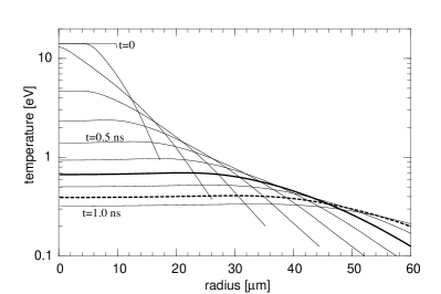
Figure 4: Hydrodynamic simulation of the density (left) and temperature (right) profiles of an expanding hydrogen microplasma starting from $n_{\mathrm{liq}}=4.5\cdot 10^{22}\,\mathrm{cm}^{-3}$ and $T=14\,\mathrm{eV}$. The broad solid and dashed curves give the conditions after 0.7 ns and 0.9 ns. At this time, the central density has reached the density which has been obtained from the fit of the Margenau profile to the H_α and the H_β spectral line, respectively for $\tau=1000\,\mathrm{fs}$ pulselength. The corresponding temperatures at these times are close to the effective temperatures $T^{\mathrm{eff}}_{\alpha\beta}\simeq 1\,\mathrm{eV}$ and $T^{\mathrm{eff}}_{\beta\gamma}\simeq 0.5\,\mathrm{eV}$ obtained from the spectra, see Tab. 1.

Fig. 4 shows the number density and temperature profiles. The uppermost curve corresponds to $t=0\,\mathrm{ns}$, while the last curve is taken at $t=1\,\mathrm{ns}$. Both parameters $n(r,t)$ and $T(r,t)$ show a fast decline in the center of the droplet. The density decreases by a factor of 10 every 300 ps. Secondly, all profiles are nearly constant over several tens of micrometers starting from the center and decrease sharply when approaching the rim of the droplet. Therefore, the central values $n(r=0,t)$ and $T(r=0,t)$ can be taken as representative values for the whole droplet. The temporal evolution of the central number density and temperature is shown in Fig. 5.

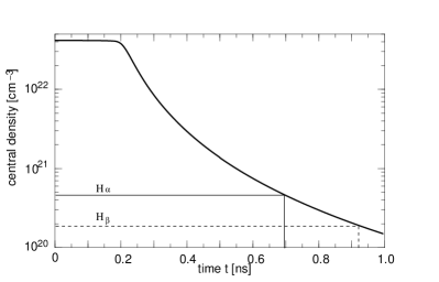
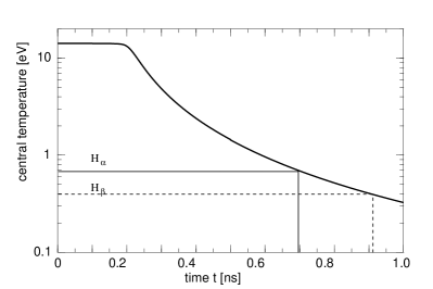
Figure 5: Temporal evolution of central density $n(r=0,t)$ (left) and temperature $T(r=0,t)$ (right), given as bold solid lines. Narrow solid line: central parameters after 0.7 ns, i.e. at the time, when the density obtained in the fit of the Margenau profile to the H_α line, $n^{(\alpha)}_{\mathrm{atom}}=4.5\cdot 10^{20}\,\mathrm{cm}^{-3}$ is reached. Dashed line: the same for H_β.

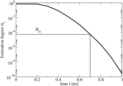
Figure 6: Ionization degree $\alpha_{e}$ as a function of time obtained from Saha equation (bold solid curve). The narrow horizontal line gives the ionization after 0.7 ns, i.e. at the time, when the central density has decreased to $n^{(\alpha)}_{\mathrm{atom}}=4.5\cdot 10^{20}\,\mathrm{cm}^{-3}$, which has been obtained as best-fit parameter with respect to the Margenau profile of the H_α spectral line.

The hydrodynamical description gives the time evolution of the excited droplet. The assumption of local thermal equilibrium may be justified on the time scale of ps for the thermalization of kinetic energies. If assuming also local ionization equilibrium, the composition during the time evolution can be calculated. The temporal behaviour of the ionization in the droplet’s center is plotted in Fig. 6. For the initial conditions $T=14\,\mathrm{eV}$ and $n_{\mathrm{liq}}=4.2\cdot 10^{22}\,\mathrm{cm}^{-3}$, we have an ionization degree $\alpha_{e}=n_{\mathrm{free}}/n=0.68$. After $t=0.7\,\mathrm{ns}$, the density and temperature have decreased so far, that $\alpha_{e}$ drops below $10^{-4}$. This corresponds to a concentration of free electrons of roughly $10^{17}\,\mathrm{cm}^{-3}$. At this density, and $T\simeq 1\,\mathrm{eV}$, the Stark effect leads to a broadening of the H_α line of 1 nm, as was discussed in Sec. III.2.2. Thus, at times larger than 0.7 ns, Stark broadening does not give a notable contribution to the width of the spectral lines.

This analysis has shown, that the emission of Balmer line radiation occurs at comparatively late times of the expansion, when the density has decreased to a certain level. This is due to the fact, that in a dense system, excited levels are not well defined due to interaction with neighbouring atoms. Both wavefunctions and atomic potentials are disturbed. In the following section we will analyse the question, which density has to be established in the system, so that excited atomic levels are defined and the corresponding radiative transition may occur.

IV.2 Occupation of excited levels

In a dense system, the potential energy of an electron in a given atom is modified by the medium Siedschlag and Rost (2005). Thus, energy eigenvalues and wave functions are changed due to screening by free charge carriers. In particular, it is well-known that bound states merge with the continuum of scattering states at high densities so that the electrons are no longer bound to a special ion, but move relatively free in the plasma as denoted by a transition from dielectric to metallic behavior Kraeft et al. (1986). Considering excited states, the dissolution occurs already at lower densities so that these excited states cannot any longer be occupied to produce a line spectrum.

We focus here to the influence of bound states in the medium to analyze at which densities the excited states are dissolved into the continuum so that no line spectra are formed. In a first approximation, we calculate the modification of the potential in the Schrödinger equation for the hydrogen atom due to the perturbing atoms in the surrounding medium. Only ground state atoms are considered, and the correlations between the electrons in the perturbing ground state with the radiating electron in the excited state are neglected. Solving the Poisson equation, the effective potential is obtained as superposition of the Coulomb potential and the potential of the neighboured atoms, which leads to a lowering of the Coulomb potential by the amount

$$\Delta V_{i}(\vec{r})=-{e^{2}\over 4\pi\epsilon_{0}|\vec{r}-\vec{R}_{i}|}e^{-2|\vec{r}-\vec{R}_{i}|/a_{B}}\left(1+{|\vec{r}-\vec{R}_{i}|\over a_{B}}\right)\,.$$ (17)

Here, $\vec{R}_{i}$ is the position of the perturbing atom. The lowering of the Coulomb potential has two effects: On the one hand, the energy level is shifted to lower energies, on the other hand, at a certain critical distance, the threshold of potential energy between neighboured atoms crosses the shifted electrons energy level, and the bound state is dissolved into the continuum. This is the case, if the distance between neighbours comes into the range of the extension of the electrons wave-function. We assume a closely packed configuration where the radiating atom is surrounded by 12 perturbing next neighbours. The shift of the energy levels with principal quantum numbers $n$ = 3 and 4 has been evaluated in first order of perturbation theory and can be given in an analytical form. Results for the shift as a function of the interatomic distance are given in Fig. 7(a).

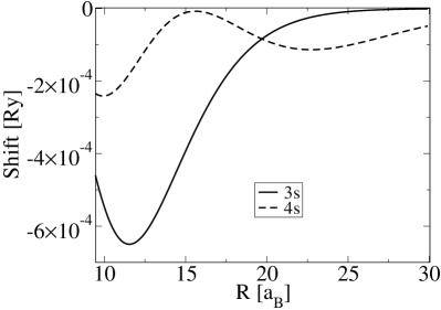
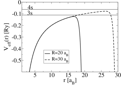
Figure 7: (a) Energy shift of 3s and 4s levels as a function of the distance $R$ to the next neighbouring atom.
(b) Effective potential due to the overlap between the radiator’s Coulomb potential and the screened potential of the next neighbouring atom in its ground state. Results are shown for two different values of the interatomic distance $R=20a_{\mathrm{B}}$ (bold curve) and $R=30\,a_{\mathrm{B}}$ (dashed curve). The perturbed 3s ($R=20\,a_{\mathrm{B}}$) and 4s ($R=30\,a_{\mathrm{B}}$) energies are given as narrow lines.

In Fig 7(b) we give the potential energy $V(r)$ in the direction to a next neighbour for two different distances, together with the corresponding shift of the energy levels with $n$ = 3 and $n=4$. As can be seen, the bound state disappears at a critical distance $R_{c}^{(n)}$ where the threshold energy becomes lower than the binding energy, and the electron is no longer bound to the central ion, but escapes the effective potential and moves relatively freely within the cluster.

From the critical distance $R_{c}^{(n)}$, one can then infer the “critical” density $n_{c}^{(n)}$ that has to be established in the expanding system, before the upper level $n$ of the considered transition can exist, i.e. before the corresponding spectral line can occur. In this way, we obtained for the second excited level, relevant for the H_α transition, a “critical” density of $n^{(\alpha)}_{c}\simeq 1.24\cdot 10^{21}\,\mathrm{cm}^{-3}$. This value for $n_{c}$ is by a factor of two larger than the value $n^{(\alpha)}_{\mathrm{atom}}=4.5\cdot 10^{20}\,\mathrm{cm}^{-3}$ obtained from the fit of the $H_{\alpha}$ line to the line shape due to van der Waals interaction, cf. Fig. 2(a).

It has to emphasized in this context, that these are exploratory calculations to estimate the region of density where well-defined excited energy levels of the radiating atom can exist. A more detailed calculation should include electronic correlations between radiator and perturber which have been neglected in the calculation of the perturbing potential. The account for correlation and exchange effects will modify the potential and the critical density. In addition, we considered only a perturbing atom at mean distance, neglecting any fluctuations in configurations. On the other hand, the experimental spectra are time integrated measurements and hence the density has to be interpreted as a mean value, averaged over the whole exposure time. At the moment the radiation starts, the density might in fact be larger than the value inferred from the measured spectra. For $H_{\beta}$, the critical density is obtained as $n_{c}^{(\beta)}\simeq 2.66\cdot 10^{20}\,\mathrm{cm}^{-3}$, which also exceeds the fit parameter for the H_β line ($n^{(\beta)}_{\mathrm{atom}}=1.8\cdot 10^{20}\,\mathrm{cm}^{-3}$) for the same reasons as given above for the case of the H_α line (cf. Fig. 2(b)).

In conclusion, the experimental Balmer spectra are not characteristic for the first stage of the laser excitation of the cluster, because the density of hydrogen in the condensed state is too high to form well-defined excited atomic levels with the corresponding principal quantum numbers. Such levels appear only during the process of expansion and may be used as a signal to infer the state of the microplasma at the corresponding time stage.

IV.3 Line emission scenario

As discussed in the previous Section, the observed Balmer spectra cannot be interpreted within an equilibrium picture of the laser produced microplasma. We could not infer consistent values of plasma parameters for temperature and density. A consistent description is only possible if the time evolution of the expanding microplasma is considered as a non-equilibrium process.

We follow the dynamical expansion of the laser excited hydrogen droplet as given by the hydrodynamical calculation. First, the time evolution of the density is considered, with account to the effective densities derived from the measured line profiles. Thereby, one can determine the time at which the H_α line appears, i.e. where the inferred density $n^{(\alpha)}_{\mathrm{atom}}=4.5\cdot 10^{20}\,\mathrm{cm}^{-3}$ is reached. Starting with the excitation temperature $T=14$ eV after the short-pulse laser excitation, this density is established after 0.7 ns. The corresponding temperature obtained from the hydrocode MULTI is $T=0.65$ eV and is in reasonable agreement with the estimate for $T^{\mathrm{eff}}_{\alpha\beta}$ given in Sec. III.2.2. Thus, the H_α line profile reflects the state of the expanding microplasma after 0.7 ns. In the case of the H_β we observe the following: From the van der Waals fit to the data, cf. Fig. 2(b), $n^{(\beta)}_{\mathrm{atom}}=1.8\cdot 10^{20}\,\mathrm{cm}^{-3}$ was obtained, which is reached in the hydrodynamic simulation after $t\simeq 0.9\,\mathrm{ns}$. The temperature is $T\simeq 0.4\,\mathrm{eV}$ at that moment, which is close to the value $0.5\,\mathrm{eV}$ obtained for $T^{\mathrm{eff}}_{\beta\gamma}$, cf. Tab. 1. H_β thus gives us information about the state of the droplet at $t\simeq 0.9\,\mathrm{ns}$.

Second, as for the empirically determined plasma parameters, the critical densities for H_α and H_β as discussed in Sec. IV.2, have to be compared to the results of the hydrodynamic simulation. The central density of the droplet decreases to the critical density for H_α to appear, $n_{c}^{(\alpha)}=1.24\cdot 10^{21}\,\mathrm{cm}^{-3}$ after 0.45 ns. After the same time, the temperature at the center of the droplet has decreased to 1.3 eV, which is in good agreement with the value 1 eV inferred from $T^{\mathrm{eff}}_{\alpha\beta}$. The critical density for H_β, $n_{c}^{(\beta)}=2.66\cdot 10^{20}\,\mathrm{cm}^{-3}$ is reached after 0.8 ns. The central temperature is 0.5 eV at that moment, which again coincides well with the value 0.5 eV as obtained from $T^{\mathrm{eff}}_{\beta\gamma}$, cf. Tab. 1.

This analysis shows, that the droplet in fact undergoes a complex dynamical evolution. Using hydrocodes to model the droplets history, we can understand the experimental observations. The initial temperature of $14$ eV is consistent with the observed temperatures and densities established at later times of the evolution. The line radiation obviously stems from relatively late times. What happens before line radiation appears? At the initial conditions of $n_{\mathrm{atom}}=n_{\mathrm{liq}}=4.2\cdot 10^{22}\,\mathrm{cm}^{-3}$ and $T=14\,\mathrm{eV}$, the ionization of the droplet was calculated as $\alpha_{e}=68\%$, solving Saha’s equation, cf. Fig. 6. The plasma emission is thus dominated by continuum radiation (free-free and free-bound transitions). However, since the detector integrates over the whole evolution of the plasma, only a nearly constant background remains in the spectrum from this early stage of the evolution. As the ionization decreases, bound states begin to form and line radiation occurs. However, for a given spectral line, both upper and lower level of the corresponding transition have to be well defined. To this end, the density has to fall below a certain value, in order to allow for the excited energy level to appear underneath the effective potential in the dense medium.

Considering the time scales for the expansion of the cluster of the order $10^{-9}\,\mathrm{s}$ according to the hydrodynamical calculations, the local thermodynamic equilibrium can be assumed, and the life time of the excited states of the order $10^{-11}\,\mathrm{s}$ is short compared with the evolution of the microplasma. In a more rigorous approach, the variation of temperature and density in space and time should be accounted for to synthesize the spectra.

V Conclusions

We found that the visible spectra can be used to get signatures for a time-resolved picture of an expanding microplasma. The line profiles allow for the determination of the microplasma’s temperature and density during its hydrodynamic expansion. We considered an energy deposition in the liquid hydrogen droplet which is sufficiently weak so that in the expanded phase most of the electrons are found in atomic bound states. Thus, the spectral line profiles are determined by van der Waals broadening. We presented a general quantum statistical approach to line profiles which allows for the unified description of charged and neutral perturbers, including density effects such as dynamical screening or strong collisions.

Although the spectra are time integrated measurements, we can use the Balmer lines as signatures for the expanding microplasma at definite values of density. A consistent scenario for the emission of Balmer lines has been given. To follow the time evolution of an excited droplet more directly, time resolved spectra have to be analyzed. Possibly, this can be achieved with pump-probe experiments and/or stimulated emission measurements.

Appendix A Green function approach to the polarization function

The general expression for the single state contribution $\Pi_{1}(\vec{k},\omega)$ to the polarization function has the form

$$\Pi_{1}(\vec{k},\omega_{\mu})=\parbox{80.0pt}{\psfig{width=80.0pt}}~{}.$$ (18)

The full single-particle propagator contains the self-energy $\Sigma_{1}(\vec{p},z)$,

$$\parbox{80.0pt}{\psfig{width=80.0pt}}\,=\,\parbox{80.0pt}{\psfig{width=80.0pt}}\,+\,\parbox{80.0pt}{\psfig{width=80.0pt}}~{}.$$ (19)

The vertex $\Gamma$ describes the coupling to the electromagnetic field and can also be expressed in terms of an effective interaction kernel. Both quantities, self-energy $\Sigma$ and vertex $\Gamma$, have to be approximated in a consistent way. For the self-energy one has the $GW\Gamma$ approximation, given by the diagram

$$\Sigma^{GW\Gamma}(\vec{p},z_{\nu})=\parbox{80.0pt}{\psfig{width=80.0pt}}~{},$$ (20)

which is a self-consistent equation for the full propagator, the full vertex $\Gamma$, as well as for the screened interaction potential $W$,

$$W(\vec{k},\omega_{\mu}) =\parbox{50.0pt}{\psfig{width=50.0pt}}=\parbox{40.0pt}{\psfig{width=40.0pt}}+\parbox{80.0pt}{\psfig{width=80.0pt}}=\frac{V(\vec{k})}{1-V(\vec{k})\Pi(\vec{k},\omega_{\mu})}~{},$$ (21)

while the vertex function $\Gamma$ is the solution of the Bethe-Salpeter equation, given in diagrammatic form by

$$\parbox{40.0pt}{\psfig{width=40.0pt}}\,\,\,=\,\parbox{40.0pt}{\psfig{width=40.0pt}}\,\,\,+\,\parbox{80.0pt}{\psfig{width=80.0pt}}~{}.$$ (22)

Solving Eq. (20) and Eq. (22) simultaneously is a formidable task. Considerable simplification of the problem is obtained by replacing the full vertex $\Gamma$ in Eq. (20) by the bare vertex $\Gamma^{(0)}$. This is the so-called $GW$ approximation,

$$\Sigma^{GW}(\vec{p},z_{\nu})=\parbox{80.0pt}{\psfig{width=80.0pt}}~{}.$$ (23)

The $GW$ approximation is well studied in condensed matter physics. It also describes bremsstrahlung an can be further improved accounting for plasma effects, see Ref. C. Fortmann, G. Röpke, and A. Wierling, physics/0610262, accepted for publication in Contrib. Plasma Phys. .

The two-particle contribution $\Pi_{2}(\vec{k},\omega)$ to the polarization function is described in analogy to Eq. (18),

$$\Pi_{2}(\vec{k},\omega_{\mu})=\parbox{100.0pt}{\includegraphics[width=100.0pt]{eps/feyn_Pi_2_GGV.eps}}~{},$$ (24)

where we have the full two-particle propagator

$$G_{2}(\alpha\vec{P},\Omega_{\lambda}) =\parbox{80.0pt}{\psfig{width=80.0pt}}=\parbox{80.0pt}{\psfig{width=80.0pt}}+\parbox{100.0pt}{\psfig{width=100.0pt}}$$

$$=\frac{1}{\Omega_{\lambda}-E_{\alpha\vec{P}}-\Sigma_{2}(\alpha\vec{P},\Omega_{\lambda})},$$ (25)

with the two-particle self-energy $\Sigma_{2}(\alpha\vec{P},\Omega_{\lambda})$,

$$\Sigma_{2}(\alpha\vec{P},\Omega_{\lambda})=\parbox{80.0pt}{\psfig{width=80.0pt}}$$ (26)

and the vertex follows from an equation in analogy to Eq. (22)

$$\parbox{50.0pt}{\psfig{width=50.0pt}}=\parbox{50.0pt}{\psfig{width=50.0pt}}+\parbox{100.0pt}{\psfig{width=100.0pt}}~{}.$$ (27)

For the polarization function which defines the screened interaction used in the two-particle self-energy Eq. (26), we perform the cluster decomposition as outlined in Sec. II. In the impact-approximation, we replace the full screened interaction by the first non-ideal term in the iteration of Eq. (21). Diagrammatically, the two-particle self-energy in impact-approximation reads

$$\Sigma^{\mathrm{imp}}(\alpha\vec{P},\Omega_{\lambda})=\parbox{80.0pt}{\psfig{width=100.0pt}}$$ (28)

Note that one has to take into account that double counting has to be avoided so that scattering states in $\Pi_{2}(\vec{k},\omega)$ should not interfer with contributions from $\Pi_{1}(\vec{k},\omega)$. Important are the account of bound states in $\Pi_{2}(\vec{k},\omega)$.

The higher order corrections to the full vertex $M(\vec{q})$ can be shown to effectively reduce the two-particle self-energy Günter (1995) by the amount $i\Gamma^{v}$. After analytic continuation $\omega_{\mu}\to\omega+i0^{+}$ to real frequencies, we obtain

$$\Pi_{2}(\vec{k},\omega)=4\sum_{\alpha_{1}\alpha_{2},\vec{P}}\left|M_{\alpha_{1}\alpha_{2}}^{(0)}(\vec{k})\right|^{2}\left(g(E^{(0)}_{\alpha_{1}\vec{P}})-g(E^{(0)}_{\alpha_{2}\vec{P}-\vec{k}})\right)\\ \times\bigg{[}\omega-E^{(0)}_{\alpha_{2}\vec{P}-\vec{k}}+E^{(0)}_{\alpha_{1}\vec{P}}-\mathrm{Re}\,\left\{\Sigma_{\alpha_{2}}(E^{(0)}_{\alpha_{1}\vec{P}}+\omega)-\Sigma_{\alpha_{1}}(E^{(0)}_{\alpha_{1}\vec{P}})\right\}+i\mathrm{Im}\,\left\{\Sigma_{\alpha_{2}}(E^{(0)}_{\alpha_{1}\vec{P}}+\omega)+\Sigma_{\alpha_{1}}(E^{(0)}_{\alpha_{1}\vec{P}})\right\}+i\Gamma^{v}\bigg{]}^{-1}~{}.$$ (29)

Note, that the dependance on $\omega$ is neglected in the self-energy of the lower energy level Günter (1995). Neglecting the self-energy and the effective vertex in Eq. (29), we arrive at Eq. (3).

Appendix B Bound state contribution to the two-particle self-energy

The interaction between two atoms in state $\left|\alpha_{1}\!\right.\rangle$ and $\left|\alpha_{2}\!\right.\rangle$, moving with momentum $\vec{P}_{1}$ and $\vec{P}_{2}$ respectively, and carrying Matsubara frequencies $\Omega_{\lambda}$ and $\Omega_{\kappa}$, upon exchange of momentum $\vec{k}$ is given by the following diagram:

$$V_{\alpha_{1},\alpha_{2}}(\vec{P}_{1},\Omega_{\lambda},\vec{P}_{2},\Omega_{\kappa},\vec{k},\omega_{\mu})=\parbox{100.0pt}{\psfig{width=100.0pt}}$$ (30)

$$=\sum_{\alpha_{3},\alpha_{4}\vec{k}^{\prime}}M^{(0)}_{\alpha_{1}\alpha_{3}}(\vec{k}^{\prime})M^{(0)}_{\alpha_{3}\alpha_{1}}(\vec{k}-\vec{k}^{\prime})M^{(0)}_{\alpha_{2}\alpha_{4}}(-\vec{k}^{\prime})M^{(0)}_{\alpha_{4}\alpha_{2}}(\vec{k}+\vec{k}^{\prime})V_{\vec{k}^{\prime}}V_{\vec{k}-\vec{k}^{\prime}}\left[\Omega_{\lambda}+\Omega_{\kappa}-E^{(0)}_{\alpha_{3}\vec{P}_{1}+\vec{k}^{\prime}}-E^{(0)}_{\alpha_{4}\vec{P}_{2}-\vec{k}^{\prime}}\right]^{-1}~{},$$ (31)

with the unscreened Coulomb propagator $V_{\vec{k}}=-1/\epsilon_{0}k^{2}\Omega_{0}$. Due to the ion’s heavy mass, we neglect the transfer momentum $\vec{k}$ in the intermediate propagator as well as the kinetic energy $\hbar^{2}P^{2}/2M$. Replacing the Matsubara frequencies $\Omega_{\lambda}$ and $\Omega_{\kappa}$ by their on-shell values, we can perform the summations over momenta in Eq. (4) and arrive at the familiar expression Eq. (7).

Appendix C Calculation of the interaction strength

The expression Eq. (8) has to be evaluated. We rewrite it as

$$\begin{split}V^{\mathrm{vdW}}_{\alpha_{1},\alpha_{2}}(R)&=-\frac{C_{6}(\alpha_{1},\alpha_{2})}{R^{6}}\\ &=-\frac{e^{4}}{(4\pi\epsilon_{0})^{2}R^{6}}\sum_{\alpha_{3}\alpha_{4}}{}^{{}^{\prime}}\frac{\left|\langle\alpha_{1}\alpha_{2}\left|\mathrm{W}\right|\alpha_{3}\alpha_{4}\rangle\right|^{2}}{E^{(0)}_{\alpha_{1}}+E^{(0)}_{\alpha_{2}}-E^{(0)}_{\alpha_{3}}-E^{(0)}_{\alpha_{4}}}~{}.\end{split}$$ (32)

The primed sum indicates summation only over states, which assure a finite denominator.

Henceforth, we assume one atom in an excited state $\alpha_{1}=n_{1}l_{1},n_{1}=2,3,4,\dots$, and the second atom in its ground state, $\alpha_{2}\equiv 0$. The denominator is dominated by the term $E^{(0)}_{\alpha_{1}}+E^{(0)}_{\alpha_{2}}=-\mathrm{Ry}(1+1/n_{1}^{2})$. Eq. (32) becomes

$$C_{6}(\alpha_{1},0) =\left(\frac{e^{2}}{4\pi\epsilon_{0}}\right)^{2}\frac{1}{\left(1+1/n_{1}^{2}\right)\mathrm{Ry}}\sum_{\alpha_{3}\alpha_{4}}{}^{{}^{\prime}}\left|\langle\alpha_{1}0\left|\mathrm{W}\right|\alpha_{3}\alpha_{4}\rangle\right|^{2}$$ (33)

$$=\left(\frac{e^{2}}{4\pi\epsilon_{0}}\right)^{2}\frac{1}{\left(1+1/n_{1}^{2}\right)\mathrm{Ry}}\sum_{\alpha_{3}\alpha_{4}}\langle\alpha_{1}0\left|\mathrm{W}\right|\alpha_{3}\alpha_{4}\rangle\langle\alpha_{3}\alpha_{4}\left|\mathrm{W}\right|\alpha_{1}0\rangle-\left|\langle\alpha_{1}0\left|\mathrm{W}\right|\alpha_{1}0\rangle\right|^{2}$$ (34)

$$=\left(\frac{e^{2}}{4\pi\epsilon_{0}}\right)^{2}\frac{1}{\left(1+1/n_{1}^{2}\right)\mathrm{Ry}}\langle\alpha_{1}0\left|\mathrm{W}^{2}\right|\alpha_{1}0\rangle~{}.$$ (35)

The diagonal matrix element of $\mathrm{W}$ vanishes for atoms with no permanent electric dipole moment. Chosing the nucleus-nucleus axis parallel to the $x$-axis of the coordinate system, the operator $\mathrm{W}$ reads

$$\mathrm{W}=\mathrm{y}_{1}\mathrm{y}_{2}+\mathrm{z_{1}}\mathrm{z}_{2}-2\mathrm{x}_{1}\mathrm{x}_{2}~{}.$$ (36)

Since the expectation values of any coordinate $x,y$ or $z$ vanishes, e.g. $\langle\alpha_{1}0\left|\mathrm{r_{i}}\right|\alpha_{1}0\rangle=0,\,i=1,2,3$, the mixed terms in $\mathrm{W}^{2}$ vanish. We obtain

$$C_{6}(\alpha_{1},0) =\left(\frac{e^{2}}{4\pi\epsilon_{0}}\right)^{2}\frac{1}{\left(1+1/n_{1}^{2}\right)\mathrm{Ry}}\langle\alpha_{1}0\left|\mathrm{y_{1}^{2}y_{2}^{2}+z_{1}^{2}z_{2}^{2}+4x_{1}^{2}x_{2}^{2}}\right|\alpha_{1}0\rangle$$ (37)

$$=\left(\frac{e^{2}}{4\pi\epsilon_{0}}\right)^{2}\frac{1}{\left(1+1/n_{1}^{2}\right)\mathrm{Ry}}\Big{[}$$ (38)

$$\langle 0\left|\mathrm{y_{1}^{2}}\right|0\rangle\langle\alpha_{1}\left|\mathrm{y_{2}^{2}}\right|\alpha_{1}\rangle+\langle 0\left|\mathrm{z_{1}^{2}}\right|0\rangle\langle\alpha_{1}\left|\mathrm{z_{2}^{2}}\right|\alpha_{1}\rangle+4\langle 0\left|\mathrm{x_{1}^{2}}\right|0\rangle\langle\alpha_{1}\left|\mathrm{x_{2}^{2}}\right|\alpha_{1}\rangle\Big{]}~{},$$ (39)

and with

$$\langle r_{i}^{2}\rangle=\frac{1}{3}\langle r^{2}\rangle$$ (40)

$$C_{6}(\alpha_{1},0) =\left(\frac{e^{2}}{4\pi\epsilon_{0}}\right)^{2}\frac{1}{\left(1+1/n_{1}^{2}\right)\mathrm{Ry}}\frac{2}{3}\langle 0\!\left|\,\mathrm{r}^{2}\,\right|\!0\rangle\langle\alpha_{1}\!\left|\,\mathrm{r^{2}}\,\right|\!\alpha_{1}\rangle~{}.$$ (41)

Using

$$\langle nl\!\left|\,\mathrm{r^{2}}\,\right|\!nl\rangle=\frac{n^{2}a_{\mathrm{B}}^{2}}{2}\left[5n^{2}+1-3l(l+1)\right]~{},$$ (42)

we finally obtain Eq. (10).

Note, that for the case, that the first atom is also in its ground state, i.e. $\alpha\equiv 0$, $C_{6}(0,0)=12$ is obtained. The difference to the London-Eisenschitz result 12.94 is due to the approximative treatment of the denominator in Eq. (32) in the calculation presented above. For excited states, which are considered in this work, this contribution becomes negligible.

Appendix D Evaluation of the van der Waals profile

We start with the general form of expression (7), i.e. the intensity distribution of a given spectral line, due to interaction between the radiator, which is in state $\left|\,i\,\right.\rangle$ before the transition and in state $\left|\,f\,\right.\rangle$ after the transition and the perturber $i,i=1\dots N$ in state $\left|n_{i}\!\right.\rangle$ . It is obtained by performing an averaging procedure over the distribution of the $N$ perturbing atoms,

$$I_{if}(\Delta\omega)=\int\mathrm{d}^{3}\vec{r}_{1}\int\mathrm{d}^{3}\vec{r}_{2}\ldots\int\mathrm{d}\vec{r}_{N}P_{N}(\vec{r}_{1},\vec{r}_{2},\ldots,\vec{r}_{N})\,\delta\left(\sum_{j=1}^{N}V_{i\alpha_{j}}(r_{j})-V_{f\alpha_{j}}(r_{j})-\Delta\omega\right)~{}.$$ (43)

Here, $P_{N}(\vec{r}_{1},\ldots\vec{r}_{N})$ is the probability density for having atom 1 in the volume element $\mathrm{d}^{3}\vec{r}_{1}$ at $\vec{r}_{1}$, atom 2 in the volume element $\mathrm{d}^{3}\vec{r}_{2}$ at $\vec{r}_{2}$, and so forth. In can be expanded in a cluster decomposition as

$$P_{N}(\vec{r}_{1},\vec{r}_{2},\ldots,\vec{r}_{N})=\frac{1}{V^{N}}\left(1+\sum_{j<k}g_{2}(\vec{r}_{j},\vec{r}_{k})+\sum_{j<k<l}g_{3}(\vec{r}_{j},\vec{r}_{k},\vec{r}_{l})+\dots\right)~{},$$ (44)

where the lowest non-ideal term is the pair distribution function, giving the probability to find a second particle at $\vec{r}_{k}$ if there is one particle at $\vec{r}_{j}$.

The $N^{3}$-fold integral in Eq. (43) can be evaluated using the Fourier representation of the delta function,

$$\delta(\Phi-\Delta\omega)=\frac{1}{2\pi}\int_{-\infty}^{\infty}\mathrm{d}\rho\,\mathrm{e}^{i\rho(\Phi-\Delta\omega)}~{},$$ (45)

with $\Phi=\sum_{j=1}^{N}[V_{i\alpha_{j}}(r_{j})-V_{f\alpha_{j}}(r_{j})]$. In the case of statistically independant atoms, which are all in the same quantum state $\alpha_{j}\equiv\alpha_{p}$ i.e. $P_{N}(\vec{r}_{1},\vec{r}_{2},\ldots,\vec{r}_{N})=V^{-N}$, one immediatly finds

$$I_{if}(\Delta\omega)=\frac{1}{2\pi}\left(\frac{4\pi}{V}\right)^{N}\int_{-\infty}^{\infty}\mathrm{d}\rho\,\mathrm{e}^{-i\Delta\omega\rho}\left[\int\mathrm{d}r\,r^{2}\mathrm{e}^{i\rho[V_{i,\alpha_{p}}(r)-V_{f,\alpha_{p}}(r)]}\right]^{N}~{}.$$ (46)

Using the van der Waals limit of the atom-atom potential, Eq. (9), Eq. (46) turns to

$$I^{\mathrm{vdW}}_{if}(\Delta\omega)=\frac{1}{2\pi}\left(\frac{4\pi}{V}\right)^{N}\int_{-\infty}^{\infty}\mathrm{d}\rho\,\mathrm{e}^{-i\Delta\omega\rho}\left[\int\mathrm{d}r\,r^{2}\mathrm{e}^{-i\rho C_{6}/r^{6}}\right]^{N}~{}.$$ (47)

The integration over $r$ can be rewritten in the form

$$\int_{0}^{\infty}\mathrm{d}r\,r^{2}\,\mathrm{e}^{-i\rho C_{6}/r^{6}} =\int_{0}^{\infty}\mathrm{d}r\,r^{2}\left[1-\left(1-\mathrm{e}^{-i\rho C_{6}/r^{6}}\right)\right]$$ (48)

$$=\frac{V}{4\pi}\left(1-\frac{4\pi\tilde{V}(\rho)}{V}\right)~{},$$ (49)

with $C_{6}=C_{6}(f,0)-C_{6}(i,0)$. In the thermodynamic limit, i.e. $V\to\infty,N\to\infty$, while keeping constant the density of neutrals $N/V=n_{\mathrm{atom}}=\mathrm{const}$, one obtains

$$\lim_{N\to\infty}\left(1-\frac{4\pi\tilde{V}(\rho)n_{\mathrm{atom}}}{N}\right)^{N}=\mathrm{e}^{-4\pi n_{\mathrm{atom}}\tilde{V}(\rho)}~{}.$$ (50)

For $\tilde{V}(\rho)$,

$$\tilde{V}(\rho)=\int_{0}^{\infty}\mathrm{d}r\,r^{2}\,\left(1-\mathrm{e}^{-i\rho C_{6}/r^{6}}\right)=\frac{(2\pi C_{6}\rho)^{1/2}}{6}(1-i)~{},$$ (51)

is obtained, and finally the Fourier integral Eq. (47) can be evaluated to give

$$I^{\mathrm{vdW}}_{if}(\Delta\omega)=\frac{2\pi n_{\mathrm{atom}}\sqrt{C_{6}}}{3(-\Delta\omega)^{3/2}}\mathrm{e}^{\pi C_{6}(2\pi n_{\mathrm{atom}}/3)^{2}/\Delta\omega}~{},$$ (52)

which corresponds to Eq. (14).

References

- Flohr and Piel (1993) R. Flohr and A. Piel, Phys. Rev. Lett. 70, 1108 (1993).
- Godbert et al. (1994) L. Godbert, A. Calisti, R. Stamm, B. Talin, S. Glenzer, H.-J. Kunze, J. Nash, R. Lee, and L. Klein, Phys. Rev. E 49, 5889 (1994).
- Malyshev and Donnelly (1999) M. V. Malyshev and V. M. Donnelly, Phys. Rev. E 60, 6016 (1999).
- Tadokoro et al. (1998) M. Tadokoro, H. Hirata, N. Nakano, Z. L. Petrovic, and T. Makabe, Phys. Rev. E 57, R43 (1998).
- Soria et al. (2000) R. Soria, K. Wu, and R. W. Hunstead, Astrophys. J. 539, 445 (2000), eprint astro-ph/9911318.
- Benz (2002) A. O. Benz, Plasma Astrophysics (Kluwer Academic Publishers, 2002), 2nd ed.
- Rybicki and Lightman (1975) G. B. Rybicki and A. P. Lightman, Radiative Processes in Astrophysics (J. Wiley & Sons, New York, 1975).
- Baranger (1962) M. Baranger, in Atomic and Molecular Processes, edited by D. Bates (Academic Press, New York, 1962), chap. 13.
- Griem and Kolb (1958) H. Griem and A. Kolb, Phys. Rev. 111, 514 (1958).
- Sobelmann et al. (1981) I. I. Sobelmann, L. A. Vainshtein, and E. A. Yukov, Excitation of atoms and broadening of spectral lines, vol. 7 of Springer Ser. Chem. Phys. (Springer, Berlin, Heidelberg, New York, 1981).
- Griem (1964) H. R. Griem, Plasma Spectroscopy (McGraw-Hill, New York, 1964).
- Smith et al. (1969) E. W. Smith, J. Cooper, and C. R. Vidal, Phys. Rev. 185, 140 (1969).
- Voslamber (1969) D. Voslamber, Zs. Naturforsch. 24a, 1458 (1969).
- Günter et al. (1991) S. Günter, L. Hitzschke, and G. Röpke, Phys. Rev. A 44, 6834 (1991).
- Günter (1995) S. Günter, Optische Eigenschaften Dichter Plasmen (Habilitation thesis, Rostock, 1995).
- Röpke et al. (1981) G. Röpke, T. Seifert, and K. Kilimann, Ann. Phys. (Leipzig) 38, 381 (1981).
- Hitzschke et al. (1986) L. Hitzschke, G. Röpke, T. Seifert, and K. Kiliman, J. Phys. B 19, 2443 (1986).
- Könnies and Günter (1994) A. Könnies and S. Günter, J. Quant. Spectrosc. Radiat. Transfer 52, 423 (1994).
- Milosavljević and Djeniźe (2003) V. Milosavljević and S. Djeniźe, Eur. Phys. J. D 23, 385 (2003).
- Omar et al. (2006) B. Omar, S. Günter, A. Wierling, and G. Röpke, Phys. Rev. E 73, 056405 (2006).
- Wilhein et al. (1998) T. Wilhein, D. Altenbernd, U. Teubner, E. Förster, R. Häßner, W. Theobald, and R. Sauerbrey, J. Opt. Soc. Am. B 15, 1235 (1998).
- Sorge et al. (2000) S. Sorge, A. Wierling, G. Röpke, W. Theobald, R. Sauerbrey, and T. Wilhein, J. Phys. B 33, 2983 (2000).
- Eisenschitz and London (1930) R. Eisenschitz and F. London, Z. Physik 60, 491 (1930).
- Margenau (1935) H. Margenau, Phys. Rev. 48, 755 (1935).
- Traving (1995) G. Traving, in Plasma Diagnostics, edited by W. Lochte-Holtgreven (AIP Press, New York, 1995), chap. 2, p. 66.
- Walkup et al. (1984) R. Walkup, B. Stewart, and D. E. Pritchard, Phys. Rev. A 29, 169 (1984).
- Ditmire et al. (1996) T. Ditmire, T. Donnelly, A. M. Rubenchik, R. W. Falcone, and M. D. Perry, Phys. Rev. A 53, 3379 (1996).
- Döppner et al. (2005) T. Döppner, T. Fennel, T. Diederich, J. Tiggesbäumker, and K.-H. Meiwes-Broer, Phys. Rev. Lett. 94, 013401 (2005).
- Kim et al. (2003) K. Y. Kim, I. Alexeev, E. Parra, and H. M. Milchberg, Phys. Rev. Lett. 90, 23401 (2003).
- Fan et al. (2000) J. Fan, E. Parra, I. Alexeev, , K. Y. Kim, S. J. McNaught, H. M. Milchberg, L. Y. Margolin, and L. N. Pyatnistkii, Phys. Rev. E 62, R7603 (2000).
- Schnürer et al. (2001) M. Schnürer, S. Ter-Avetisyan, H. Stiel, U. Vogt, W. Radloff, M. Kalashnikov, W. Sandner, and P. V. Nickles, Eur. Phys. J. D 14, 331 (2001).
- Düsterer et al. (2001) S. Düsterer, H. Schwoerer, W. Ziegler, C. Ziener, and R. Sauerbrey, Appl. Phys. B 73, 693 (2001).
- Madison et al. (2004) K. W. Madison, P. K. Patel, M. Allen, D. Price, R. Fitzpatrick, and T. Ditmire, Phys. Rev. A 70, 053201 (2004).
- Nordhage et al. (2005) O. Nordhage, Z.-K. Lib, C.-J. Fridén, G. Normanc, and U. Wiedner, Nucl. Instr. Meth. Phys. Res. A 546, 391 (2005).
- Hansen et al. (2005) S. B. Hansen, K. B. Fournier, A. Y. Faenov, A. I. Magunov, T. A. Pikuz, I. Y. Skobelev, Y. Fukuda, Y. Akahane, M. Aoyama, N. Inoue, et al., Phys. Rev. E 71, 016408 (2005).
- Anand et al. (2005) M. Anand, C. P. Safvan, and M. Krishnamurthy, Appl. Phys. B 81, 469 (2005).
- Anand et al. (2006) M. Anand, P. Gibbon, and M. Krishnamurthy, Opt. Expr. 14, 5502 (2006).
- Zweiback et al. (2000a) J. Zweiback, T. Ditmire, and M. Perry, Opt. Expr. 6, 236 (2000a).
- Liu et al. (2006) J. Liu, C. Wang, B. Liu, , B. Shuai, W. Wang, Y. Cai, H. Li, G. Ni, R. Li, et al., Phys. Rev. A 73, 033201 (2006).
- Röpke and Der (1979) G. Röpke and R. Der, phys. stat. sol. (b) 92, 501 (1979).
- Mahan (1981) G. D. Mahan, Many-Particle Physics (Plenum Press, New York and London, 1981), 2nd ed.
- Wierling et al. (2001) A. Wierling, T. Millat, G. Röpke, R. Redmer, and H. Reinholz, Phys. Plasmas 8, 3810 (2001).
- (43) C. Fortmann, G. Röpke, and A. Wierling, physics/0610262, accepted for publication in Contrib. Plasma Phys.
- (44) To keep the notation short, we denote the ground state of an atom by . For hydrogen atoms, this has to be read as .
- Lochte-Holtgreven (1995) W. Lochte-Holtgreven, in Plasma Diagnostics, edited by W. Lochte-Holtgreven (AIP Press, New York, 1995), chap. 3, p. 135.
- (46) We use the normal distribution with , such that is the full width at half maximum of the distribution .
- Eidmann et al. (2000) K. Eidmann, J. Meyer-ter-Vehn, T. Schlegel, and S. Hüller, Phys. Rev. E 62, 1202 (2000).
- Ramis et al. (1988) R. Ramis et al., Comp. Phys. Comm. 49, 474 (1988).
- Ramis et al. (2004) R. Ramis et al., Nucl. Fusion 44, 720 (2004).
- Zweiback et al. (2000b) J. Zweiback, R. A. Smith, T. E. Cowan, G. Hays, K. B. Wharton, V. P. Yanovsky, and T. Ditmire, Phys. Rev. Lett. 84, 2634 (2000b).
- Siedschlag and Rost (2005) C. Siedschlag and J. M. Rost, Phys. Rev. A 71, 031401(R) (2005).
- Kraeft et al. (1986) W. D. Kraeft, D. Kremp, W. Ebeling, and G. Röpke, Statistics of Charged Particle Systems (Akademie-Verlag, Berlin, 1986).