INSTITUT NATIONAL DE RECHERCHE EN INFORMATIQUE ET EN AUTOMATIQUE

Belief Propagation and Bethe approximation for Traffic Prediction
Cyril Furtlehner — Jean-Marc Lasgouttes — Arnaud de La FortelleN° 6144
Mars 2007

Abstract: We define and study an inference algorithm based on “belief propagation” (BP) and the Bethe approximation. The idea is to encode into a graph an a priori information composed of correlations or marginal probabilities of variables, and to use a message passing procedure to estimate the actual state from some extra real-time information. This method is originally designed for traffic prediction and is particularly suitable in settings where the only information available is floating car data. We propose a discretized traffic description, based on the Ising model of statistical physics, in order to both reconstruct and predict the traffic in real time. General properties of BP are addressed in this context. In particular, a detailed study of stability is proposed with respect to the a priori data and the graph topology. The behavior of the algorithm is illustrated by numerical studies on a simple traffic toy model. How this approach can be generalized to encode superposition of many traffic patterns is discussed.

Propagation de croyances et approximation de Bethe pour la prédiction de trafic

Résumé : On définit et étudie un algorithme de reconstruction utilisant l’algorithme « Belief Propagation » (propagation de croyances, BP) et l’approximation de Bethe. L’idée est d’encoder dans un graphe des données a priori composées de corrélations ou de lois marginales et d’utiliser une procédure de passage de messages pour estimer l’état réel à partir d’informations temps-réel. Cette méthode, développée pour des besoins de prédiction de trafic, est particulièrement adaptée au cas où la seule information disponible provient de véhicules sonde (Floating Car Data). Nous proposons une discrétisation binaire du trafic s’appuyant sur le modèle d’Ising de physique statistique, permettant de reconstruire et de prédire le trafic en temps réel. Des propriétés générales de l’algorithme BP sont discutées dans ce contexte. En particulier une étude détaillée des propriétés de stabilité fonction des données a priori et de la topologie du graphe est fournie. Une étude numérique sur un modèle de trafic simplifié permet d’illustrer le fonctionnement de l’algorithme. La façon de généraliser cette approche pour encoder une superposition de plusieurs états de trafic est discutée.

Mots-clés : propagation de croyances, approximation de Bethe, reconstruction de trafic, prédiction, systèmes de transport intelligent, véhicules traceurs

1 Introduction

With an estimated $1$% GDP cost in the European Union (i.e. more than hundred billions euros), congestion is not only a time waste for drivers and an environmental challenge, but also an economic issue. This is why the European commission financed the REACT project, where new traffic prediction models have been developed. These predictions are to be used to inform the public and possibly to regulate the traffic.

Today, some urban and inter-urban areas have traffic management and advice systems that collect data from stationary sensors, analyze them, and post notices about road conditions ahead and recommended speed limits on display signs located at various points along specific routes. However, these systems are not available everywhere and they are virtually non-existent on rural areas. With rural road crashes accounting for more than $60$% of all road fatalities in OECD (Organization for Economic Cooperation and Development) countries, the need for a system that can cover these roads is compelling if a significant reduction in traffic deaths is to be achievable.

The REACT project combines a traditional traffic prediction approach on equipped motorways with an innovative approach on non-equipped roads. The idea is to obtain floating car data from a fleet of probe vehicles and reconstruct the traffic conditions from this partial information. To understand why it is not possible to fuse these two parts, we have to go a bit more into prediction algorithms details.

Two types of approaches are usually distinguished, namely data driven (application of statistical models to a large amount of data, for example regression analysis) and model based (simulation or mathematical models explaining the traffic patterns). As we stated before, the choice is largely led by the availability of data. In our case, since little data is available on non-equipped roads (only the equipped vehicles driving along the observed roads), the model driven approach is the only feasible one. For more information about traffic prediction methods, we refer the reader to [1, 13, 14].

Most current traffic models are deterministic, described either at a macroscopic level by a set of differential equations linking variables such as flow and density, or by Newton’s law at a microscopic level where each individual car is considered. Intermediate descriptions are essentially kinetic models, like for example cellular automata [11], which are very well adapted to freeway traffic modeling and adapted to some extent to urban traffic modeling [4]. Traffic flow models are quite adapted and efficient on motorways where fluid approximation of the traffic is reasonable; they tend to fail for cities or rural roads. The reason is that the velocity flow field is subject to much greater fluctuations induced by the nature of the network (presence of intersections and short distance between two intersections) than by the traffic itself. These fluctuations are both spatial and temporal (a red or green traffic light at a cross-road, a road-work, etc). There is no local stationary regime for the velocity, the dynamics are dominated by the fluctuations.

We propose in this paper a hybrid approach in the continuation of [5], by taking full advantage of the statistical nature of the information, in combination with a stochastic modeling of traffic patterns. In order to reconstruct the traffic and make predictions, we propose a model—the Bethe approximation (BA)—to encode the statistical fluctuations and stochastic evolution of the traffic and an algorithm—the belief propagation (BP) algorithm—to decode the information. Those concepts are familiar to the computer science and statistical physics communities since it was shown [16] that the output of BP is in general the Bethe approximation [3].

The paper is organized as follows: Section 2 describes the model and its relationship to the Ising model and the Bethe approximation. The inference problem and our strategy to tackle it using the Belief Propagation algorithm are stated in Section 3. The implementation of these ideas requires some new results about the BP algorithm, which are the subject of Section 4; this concerns in particular the effect of the normalization of the messages, the parameterization of the model and the stability of the fixed points. Section 5 is devoted to implementation details of the decoding algorithm and to some numerical results illustrating the method. Finally, some new research directions are proposed in Section 6.

2 Traffic description and statistical physics

The graph onto which we apply the belief propagation procedure is made of space-time vertices that encode both a location (road link) and a time (discretized on a few minutes scale). More precisely, the set of vertices is $\mathcal{V}=\mathcal{L}\otimes\mathbb{Z}^{+}$, where $\mathcal{L}$ corresponds to the links of the network and $\mathbb{Z}^{+}$ to the time discretization. To each point $\alpha=(\ell,t)\in\mathcal{V}$, we attach an information $\tau_{\alpha}\in\{0,1\}$ indicating the state of the traffic ($1$ if congested, $0$ otherwise). Each cell is correlated to its neighbors (in time and space) and the evaluation of this local correlation determines the model. In other words, we assume that the joint probability distribution of $\tau_{\mathcal{V}}\stackrel{{\scriptstyle\mbox{\tiny def}}}{{=}}\{\tau_{\alpha},\ \alpha\in\mathcal{V}\}\in\{0,1\}^{\mathcal{V}}$ is of the form

$$p(\{\tau_{\alpha},\alpha\in\mathcal{V}\})\quad=\prod_{\alpha\in\mathcal{V}}\phi_{\alpha}(\tau_{\alpha})\prod_{(\alpha,\beta)\in\mathcal{E}}\psi_{\alpha\beta}(\tau_{\alpha},\tau_{\beta})$$ (2.1)

where $\mathcal{E}\subset\mathcal{V}^{2}$ is the set of edges, and the local correlations are encoded in the functions $\psi$ and $\phi$. $\mathcal{V}$ together with $\mathcal{E}$ describe the space-time graph $\mathcal{G}$ and $\mathcal{V}(\alpha)\subset\mathcal{V}$ denotes the set of neighbors of vertex $\alpha$.

The model described by (2.1) is actually equivalent to an Ising model [8] on $\mathcal{G}$, with arbitrary coupling between adjacent spins, the up or down orientation of each spin indicating the status of the corresponding link (Figure 2.1).

Figure 2.1: Traffic network (a) and Ising model (b) on a random graph

The homogeneous Ising model (uniform coupling constants) is a well-studied model of ferro (positive coupling) or anti-ferro (negative coupling) material in statistical physics. It displays a phase transition phenomenon with respect to the value of the coupling. At weak coupling, only one disordered state occurs, where spins are randomly distributed around a mean-zero value. Conversely, when the coupling is strong, there are two equally probable states that correspond to the onset of a macroscopic magnetization either in the up or down direction: each spin has a larger probability to be oriented in the privileged direction than in the opposite one.

From the point of view of a traffic network, this means that such a model is able to describe three possible traffic regimes: fluid (most of the spins up), congested (most of the spins down) and dense (roughly half of the links are congested). For real situations, we expect other types of congestion patterns, and we seek to associate them either to the $p$-state Potts model if we extend the binary to $p$-ary description, or to the possible states of an inhomogeneous Ising model with frustration (i.e. with possibly negative coupling parameters), referred as spin glasses in statistical physics [10]. When such a system is frustrated because some negative couplings, leading to a certain number of contradictions, a proliferation of meta-stable states occurs, which eventually scales exponentially with the size of the system.

On a simply connected graph, the knowledge of the one-vertex and two-vertices marginal probabilities is sufficient [12] to fully determine the measure (2.1).

$$p(\tau_{\mathcal{V}})=\frac{\prod_{(\alpha,\beta)\in\mathcal{E}}\hat{p}_{\alpha\beta}(\tau_{\alpha},\tau_{\beta})}{\prod_{\alpha\in\mathcal{V}}\hat{p}(\tau_{\alpha})^{q_{\alpha}-1}}=\prod_{\alpha\in\mathcal{V}}\hat{p}_{\alpha}(\tau_{\alpha})\prod_{(\alpha,\beta)\in\mathcal{E}}\frac{\hat{p}_{\alpha\beta}(\tau_{\alpha},\tau_{\beta})}{\hat{p}_{\alpha}(\tau_{\alpha})\hat{p}_{\beta}(\tau_{\beta})},$$ (2.2)

where $q_{\alpha}$ denotes the number of neighbors of $\alpha$. Since our space time graph $\mathcal{G}$ is multi-connected, this relationship between local marginals and the full joint probability measure can only be an approximation, which in the context of statistical physics is referred to as the Bethe approximation. This approximation is provided by the minimum of the so-called Bethe free energy, which, based on the form (2.2), is an approximate form of the Kullback-Leibler distance,

$$D(b(\tau_{\mathcal{V}})\|p(\tau_{\mathcal{V}}))\stackrel{{\scriptstyle\mbox{\tiny def}}}{{=}}\sum_{\tau_{\mathcal{V}}}b(\tau_{\mathcal{V}})\ln\frac{b(\tau_{\mathcal{V}})}{p(\tau_{\mathcal{V}})},$$

and which rewrites in terms of a free energy as

$$D(b(\tau_{\mathcal{V}})\|p(\tau_{\mathcal{V}}))=\mathcal{F}(b(\tau_{\mathcal{V}}))-\mathcal{F}(p(\tau_{\mathcal{V}})),$$

where

$$\mathcal{F}(b(\tau_{\mathcal{V}}))\stackrel{{\scriptstyle\mbox{\tiny def}}}{{=}}\mathcal{U}(b(\tau_{\mathcal{V}}))-\mathcal{S}(b(\tau_{\mathcal{V}})),$$ (2.3)

with the respective definitions of the energy $\mathcal{U}$ and of the entropy $\mathcal{S}$

$$\mathcal{U}(b(\tau_{\mathcal{V}})) \stackrel{{\scriptstyle\mbox{\tiny def}}}{{=}}-\sum_{(\alpha,\beta)\in\mathcal{E}}b_{\alpha\beta}(\tau_{\alpha},\tau_{\beta})\log\psi_{\alpha\beta}(\tau_{\alpha},\tau_{\beta})-\sum_{\alpha\in\mathcal{V}}b_{\alpha}(\tau_{\alpha})\log\phi_{\alpha}(\tau_{\alpha}),$$

$$\mathcal{S}(b(\tau_{\mathcal{V}})) \stackrel{{\scriptstyle\mbox{\tiny def}}}{{=}}-\sum_{(\alpha,\beta)\in\mathcal{E}}b_{\alpha\beta}(\tau_{\alpha},\tau_{\beta})\log b_{\alpha\beta}(\tau_{\alpha},\tau_{\beta})-\sum_{\alpha\in\mathcal{V}}b_{\alpha}(\tau_{\alpha})\log b_{\alpha}(\tau_{\alpha}).$$

In practice, what we retain from an Ising description is the possibility to encode a certain number of traffic patterns in a statistical physics model. This property is actually shared also by the Bethe Approximation (BA) and this is the reason for us to directly encode the traffic patterns in a BA rather than the inhomogeneous Ising model itself, based on historical data, and to avoid therefore an intermediate approximation step. BA simply provides us with a set of marginals probabilities that we try to match with the historical data. But this set, which is the result of an iterative procedure, is not necessarily unique (see for example [9]) and the proliferation of possible solutions depends on the frustration induced by the historical correlations used to define the $\psi$’s of (2.1). The setting of our model consists therefore into an optimization procedure of the matching between the set of historical values obtained from probe vehicles and the set of marginal probabilities of the BA.

The data collected from the probe vehicles is used in two different ways. The most evident one is that the data of the current day directly influences the prediction. In parallel, this data is collected over long periods (weeks or months) in order to estimate the model (2.1). Typical historical data that is accumulated is

• $\hat{p}_{\alpha}(\tau_{\alpha})$: the probability that vertex $\alpha$ is congested ($\tau_{\alpha}=1$) or not ($\tau_{\alpha}=0$);

• $\hat{p}_{\alpha\beta}(\tau_{\alpha},\tau_{\beta})$: the probability that a probe vehicle going from $\alpha$ to $\beta\in\mathcal{V}(\alpha)$ finds $\alpha$ with state $\tau_{\alpha}$ and $\beta$ with state $\tau_{\beta}$.

The edges $(\alpha,\beta)$ of the space time graph $\mathcal{G}$ are constructed based on the presence of a measured mutual information between $\alpha$ and $\beta$, which is the case when $\hat{p}_{\alpha\beta}(\tau_{\alpha},\tau_{\beta})\neq\hat{p}_{\alpha}(\tau_{\alpha})\hat{p}_{\beta}(\tau_{\beta})$.

3 The reconstruction and prediction algorithm

3.1 Statement of the inference problem

We turn now to our present work concerning an inference problem, which we set in general terms as follows: a set of observables $\tau_{\mathcal{V}}=\{\tau_{\alpha},\ \alpha\in\mathcal{V}\}$, which are stochastic variables are attached to the set $\mathcal{V}$ of vertices of a graph. For each edge $(\alpha,\beta)\in\mathcal{E}$ of the graph, an accumulation of repetitive observations allows to build the empirical marginal probabilities $\{\hat{p}_{\alpha\beta}\}$. The question is then: given the values of a subset $\tau_{\mathcal{V}^{*}}=\{\tau_{\alpha^{*}},\ \alpha^{*}\in\mathcal{V}^{*}\}$, what prediction can be made concerning $\overline{\mathcal{V}^{*}}$, the complementary set of $\mathcal{V}^{*}$ in $\mathcal{V}$?

There are two main issues:

• how to encode the historical observations (inverse problem) in an Ising model, such that its marginal probabilities on the edges coincide with the $\hat{p}_{\alpha\beta}$?

• how to decode in the most efficient manner—typically in real time—this information, in terms of conditional probabilities $P(\tau_{\alpha}|\tau_{\mathcal{V}^{*}})$?

The answer to the second question will somehow give a hint to the first one.

3.2 The belief propagation algorithm

BP is a message passing procedure, which output is a set of estimated marginal probabilities, the beliefs $b_{\alpha\beta}$ [12]. The idea of the BP algorithm is to factor the marginal probability at a given site in a product of contributions coming from neighboring sites, which are the messages. The messages sent by a vertex $\alpha$ to $\beta\in\mathcal{V}(\alpha)$ depends on the messages it received previously from other vertices:

$$m_{\alpha\to\beta}(\tau_{\beta})\leftarrow\sum_{\tau_{\alpha}\in\{0,1\}}n_{\alpha\to\beta}(\tau_{\alpha})\phi_{\alpha}(\tau_{\alpha})\psi_{\alpha\beta}(\tau_{\alpha},\tau_{\beta}),$$ (3.1)

where

$$n_{\alpha\to\beta}(\tau_{\alpha})\stackrel{{\scriptstyle\mbox{\tiny def}}}{{=}}\prod_{\gamma\in\mathcal{V}(\alpha)\setminus\{\beta\}}m_{\gamma\to\alpha}(\tau_{\alpha}).$$ (3.2)

In practice, the messages will be normalized so that

$$\sum_{\tau_{\beta}\in\{0,1\}}m_{\alpha\to\beta}(\tau_{\beta})=1.$$ (3.3)

We will come back to the effects of this in Section 4.2.

The output of the algorithm is a set of beliefs, which are an approximation of the one-vertex and two-vertices marginals of $p(\tau_{\mathcal{V}})$. The beliefs $b_{\alpha}$ are reconstructed according to

$$b_{\alpha}(\tau_{\alpha})\propto\phi_{\alpha}(\tau_{\alpha})\prod_{\beta\in\mathcal{V}(\alpha)}m_{\beta\to\alpha}(\tau_{\alpha}),$$ (3.4)

and, similarly, the belief $b_{\alpha\beta}$ of the joint probability of $(\tau_{\alpha},\tau_{\beta})$ is given by

$$b_{\alpha\beta}(\tau_{\alpha},\tau_{\beta})\propto n_{\alpha\to\beta}(\tau_{\alpha})n_{\beta\to\alpha}(\tau_{\beta})\times\phi_{\alpha}(\tau_{\alpha})\phi_{\beta}(\tau_{\beta})\psi_{\alpha\beta}(\tau_{\alpha},\tau_{\beta}).$$ (3.5)

In the formulas above and in the remainder of this paper, the proportionality symbol $\propto$ indicates that one must normalize the beliefs so that they sum to $1$.

A simple computation shows that equations (3.4) and (3.5) are compatible, since (3.1)–(3.2) imply that

$$\sum_{\tau_{\alpha}\in\{0,1\}}b_{\alpha\beta}(\tau_{\alpha},\tau_{\beta})=b_{\beta}(\tau_{\beta}).$$

It has been realized a few years ago [15] that the fixed points of the BP algorithm coincide with local minima of the Bethe free energy (2.3). This justifies that we can use this algorithm to approximate our Ising model.

We propose to use the BP algorithm for two purposes: estimation of the model parameters (the functions $\phi$ and $\psi$) from historical data and reconstruction of traffic from current data.

3.3 Setting the model with Belief Propagation

The fixed points of the BP algorithm (and therefore the Bethe approximation) allow to approximate the joint marginal probability $p_{\alpha\beta}$ when the functions $\psi_{\alpha\beta}$ and $\phi_{\alpha}$ are known. Conversely, it can provide good candidates for $\psi_{\alpha\beta}$ and $\phi_{\alpha}$ from the historical values $\hat{p}_{\alpha\beta}$ and $\hat{p}_{\alpha}$.

To set up our model, we are looking for a fixed point of the BP algorithm satisfying (3.1)–(3.2) and such that $b_{\alpha\beta}(\tau_{\alpha},\tau_{\beta})=\hat{p}_{\alpha\beta}(\tau_{\alpha},\tau_{\beta})$ and therefore $b_{\alpha}(\tau_{\alpha})=\hat{p}_{\alpha}(\tau_{\alpha})$.

It is easy to check that the following choice of $\phi$ and $\psi$,

$$\psi_{\alpha\beta}(\tau_{\alpha},\tau_{\beta}) = \frac{\hat{p}_{\alpha\beta}(\tau_{\alpha},\tau_{\beta})}{\hat{p}_{\alpha}(\tau_{\alpha})\hat{p}_{\beta}(\tau_{\beta})},$$ (3.6)

$$\phi_{\alpha}(\tau_{\alpha}) = \hat{p}_{\alpha}(\tau_{\alpha}),$$ (3.7)

leads (2.1) to coincide with (2.2). They correspond to a normalized BP fixed point for which all messages are equal to $1/2$. There is however no guarantee that this fixed point is a stable fixed point; actually, for an Ising-type system below the critical temperature, we often observe that this point is unstable (see Section 5 for the simulation results). It will be shown however in Section 4.1 that this form of $\phi$ and $\psi$ is in some sense canonical.

3.4 Traffic reconstruction and prediction

Let $\mathcal{V}^{*}$ be the set of vertices that have been visited by probe vehicles. Reconstructing traffic from the data gathered by those vehicles is equivalent to evaluating the conditional probability

$$p_{\alpha}(\tau_{\alpha}|\tau_{\mathcal{V}^{*}})=\frac{p_{\alpha,\mathcal{V}^{*}}(\tau_{\alpha},\tau_{\mathcal{V}^{*}})}{p_{\mathcal{V}^{*}}(\tau_{\mathcal{V}^{*}})},$$

where $\tau_{\mathcal{V}^{*}}$ is a shorthand notation for the set $\{\tau_{\alpha^{*}}\}_{\alpha^{*}\in\mathcal{V}^{*}}$.

The BP algorithm applies to this case if a specific rule is defined for vertices $\alpha^{*}\in\mathcal{V}^{*}$: since the value of $\tau_{\alpha^{*}}$ is known, there is no need to sum over possible values and (3.1) becomes

$$m_{\alpha^{*}\to\beta}(\tau_{\beta})\leftarrow n_{\alpha^{*}\to\beta}(\tau_{\alpha^{*}})\phi_{\alpha^{*}}(\tau_{\alpha^{*}})\psi_{\alpha^{*}\beta}(\tau_{\alpha^{*}},\tau_{\beta}).$$

The resulting algorithm is supposed to be run in real time, over a graph which corresponds to a time window (typically a few hours) centered around present time, with probe vehicle data added as it is available. In this perspective, the reconstruction and prediction operations are done simultaneously on an equal footing, the distinction being simply the time-stamp (past for reconstruction or future for prediction) of a given computed belief. The output of the previous run can be used as initial messages for a new run, in order to speedup convergence. Full re-initialization (typically a random set of initial messages) has to be performed within a time interval of the order but smaller than the time-scale of typical traffic fluctuations.

4 Some general properties of the Belief Propagation algorithm

This section contains several theoretical results on the BP algorithm. Although they are stated in the context of Section 2, most of these results can be trivially extended to a general factor graph and variables taking more than two values (transforming the Ising model into a Potts model), except possibly for Section 4.3.

4.1 Building the model from its fixed points

The particular use that we make of the Bethe approximation, as outlined in Section 3.3, means that the output of the algorithm takes precedence over the underlying Ising model, which is an unusual situation. The following propositions shows how to estimate $\phi_{\alpha}$ and $\psi_{\alpha\beta}$ from the historical values $\hat{p}_{\alpha}$ and $\hat{p}_{\alpha\beta}$.

Let us start with a direct consequence of the BP fixed point equations. The following straightforward proposition extends (2.2) to the case of a non-tree structure.

Proposition 4.1.

A set of beliefs $\{b_{\alpha},b_{\alpha\beta}\}$ corresponding to a BP fixed point of (3.1)–(3.5) always satisfies

$$p(\tau_{\mathcal{V}})=\frac{\prod_{\alpha,\beta}b_{\alpha\beta}(\tau_{\alpha},\tau_{\beta})}{\prod_{\alpha}b_{\alpha}^{q_{\alpha}-1}(\tau_{\alpha})}=\prod_{\alpha\in\mathcal{V}}b_{\alpha}(\tau_{\alpha})\prod_{(\alpha,\beta)\in\mathcal{E}}\frac{b_{\alpha\beta}(\tau_{\alpha},\tau_{\beta})}{b_{\alpha}(\tau_{\alpha})b_{\beta}(\tau_{\beta})}.$$

Proof.

This is a simple consequence of (3.4)–(3.5).  

What this proposition means is that different BP fixed points correspond to different factorizations of the joint measure (2.1). The knowledge of a set of beliefs is thus sufficient to determine the underlying Ising model and consequently the other fixed points of the algorithm.

The following proposition gives more insight on how the different components of (2.1) can be written in terms of the BP fixed points.

Proposition 4.2.

Assume that there exists a fixed point of the BP algorithm satisfying (3.1)–(3.5) and such that

$$b_{\alpha\beta}(\tau_{\alpha},\tau_{\beta})=\hat{p}_{\alpha\beta}(\tau_{\alpha},\tau_{\beta}),\text{ and therefore }b_{\alpha}(\tau_{\alpha})=\hat{p}_{\alpha}(\tau_{\alpha}).$$ (4.1)

Then the following equalities hold

$$\psi_{\alpha\beta}(\tau_{\alpha},\tau_{\beta}) = \frac{\hat{p}_{\alpha\beta}(\tau_{\alpha},\tau_{\beta})}{\hat{p}_{\alpha}(\tau_{\alpha})\hat{p}_{\beta}(\tau_{\beta})}m_{\alpha\to\beta}(\tau_{\beta})m_{\beta\to\alpha}(\tau_{\alpha}),$$ (4.2)

$$\phi_{\alpha}(\tau_{\alpha}) = \frac{\hat{p}_{\alpha}(\tau_{\alpha})}{\prod_{\beta\in\mathcal{V}(\alpha)}m_{\beta\to\alpha}(\tau_{\alpha})}.$$ (4.3)

Conversely, assume that there exist boolean functions $\mu_{\alpha\beta}(\tau_{\beta})$ such that

$$\psi_{\alpha\beta}(\tau_{\alpha},\tau_{\beta}) = \frac{\hat{p}_{\alpha\beta}(\tau_{\alpha},\tau_{\beta})}{\hat{p}_{\alpha}(\tau_{\alpha})\hat{p}_{\beta}(\tau_{\beta})}\mu_{\alpha\beta}(\tau_{\beta})\mu_{\beta\alpha}(\tau_{\alpha}),$$ (4.4)

$$\phi_{\alpha}(\tau_{\alpha}) = \frac{\hat{p}_{\alpha}(\tau_{\alpha})}{\prod_{\beta\in\mathcal{V}(\alpha)}\mu_{\beta\alpha}(\tau_{\alpha})}.$$ (4.5)

Then $m_{\alpha\to\beta}=\mu_{\alpha\beta}$ is a fixed point of the BP algorithm and (4.1) holds.

Proof.

Relation (4.2) is obtained by rewriting (3.4) and (3.5) as

$$\psi_{\alpha\beta}(\tau_{\alpha},\tau_{\beta}) = \frac{b_{\alpha\beta}(\tau_{\alpha},\tau_{\beta})}{\phi_{\alpha}(\tau_{\alpha})n_{\alpha\to\beta}(\tau_{\alpha})n_{\beta\to\alpha}(\tau_{\beta})\phi_{\beta}(\tau_{\beta})}$$ (4.6)

$$= \frac{b_{\alpha\beta}(\tau_{\alpha},\tau_{\beta})}{b_{\alpha}(\tau_{\alpha})b_{\beta}(\tau_{\beta})}m_{\alpha\to\beta}(\tau_{\beta})m_{\beta\to\alpha}(\tau_{\alpha}).$$

To prove the second assertion, the first step is to show that $\mu_{\alpha\beta}$ is a BP fixed point:

$$\sum_{\tau_{\alpha}\in\{0,1\}}\biggl{[}\prod_{\gamma\in\mathcal{V}(\alpha)\setminus\{\beta\}}\mu_{\gamma\alpha}(\tau_{\alpha})\biggr{]}\phi_{\alpha}(\tau_{\alpha})\psi_{\alpha\beta}(\tau_{\alpha},\tau_{\beta})$$

$$= \sum_{\tau_{\alpha}\in\{0,1\}}\frac{\hat{p}_{\alpha}(\tau_{\alpha})}{\mu_{\beta\alpha}(\tau_{\alpha})}\frac{\hat{p}_{\alpha\beta}(\tau_{\alpha},\tau_{\beta})}{\hat{p}_{\alpha}(\tau_{\alpha})\hat{p}_{\beta}(\tau_{\beta})}\mu_{\alpha\beta}(\tau_{\beta})\mu_{\beta\alpha}(\tau_{\alpha})$$

$$= \sum_{\tau_{\alpha}\in\{0,1\}}\frac{\hat{p}_{\alpha\beta}(\tau_{\alpha},\tau_{\beta})}{\hat{p}_{\beta}(\tau_{\beta})}\mu_{\alpha\beta}(\tau_{\beta})$$

$$= \mu_{\alpha\beta}(\tau_{\beta}).$$

For this fixed point, (3.5) reduces to (4.1), which concludes the proof of the proposition.  

While Proposition 4.2 seems to indicate that there is some leeway in choosing $\psi_{\alpha\beta}$, a proper change of variables shows that all the choices are equivalent. Let us define the following new set of messages

$$x_{\alpha\to\beta}(\tau_{\beta})\stackrel{{\scriptstyle\mbox{\tiny def}}}{{=}}\frac{m_{\alpha\to\beta}(\tau_{\beta})}{\mu_{\alpha\beta}(\tau_{\beta})}.$$

Equation (3.1) then becomes

$$x_{\alpha\to\beta}(\tau_{\beta})\mu_{\alpha\beta}(\tau_{\beta})$$

$$= \sum_{\tau_{\alpha}\in\{0,1\}}\biggl{[}\prod_{\gamma\in\mathcal{V}(\alpha)\setminus\{\beta\}}x_{\gamma\to\alpha}(\tau_{\alpha})\mu_{\gamma\alpha}(\tau_{\alpha})\biggr{]}\phi_{\alpha}(\tau_{\alpha})\psi_{\alpha\beta}(\tau_{\alpha},\tau_{\beta})$$

$$= \sum_{\tau_{\alpha}\in\{0,1\}}\biggl{[}\prod_{\gamma\in\mathcal{V}(\alpha)\setminus\{\beta\}}x_{\gamma\to\alpha}(\tau_{\alpha})\biggr{]}\frac{\hat{p}_{\alpha}(\tau_{\alpha})}{\mu_{\beta\alpha}(\tau_{\alpha})}\frac{\hat{p}_{\alpha\beta}(\tau_{\alpha},\tau_{\beta})}{\hat{p}_{\alpha}(\tau_{\alpha})\hat{p}_{\beta}(\tau_{\beta})}\mu_{\alpha\beta}(\tau_{\beta})\mu_{\beta\alpha}(\tau_{\alpha})$$

$$= \sum_{\tau_{\alpha}\in\{0,1\}}\biggl{[}\prod_{\gamma\in\mathcal{V}(\alpha)\setminus\{\beta\}}x_{\gamma\to\alpha}(\tau_{\alpha})\biggr{]}\frac{\hat{p}_{\alpha\beta}(\tau_{\alpha},\tau_{\beta})}{\hat{p}_{\beta}(\tau_{\beta})}\mu_{\alpha\beta}(\tau_{\beta}),$$

and therefore

$$x_{\alpha\to\beta}(\tau_{\beta})=\sum_{\tau_{\alpha}\in\{0,1\}}\biggl{[}\prod_{\gamma\in\mathcal{V}(\alpha)\setminus\{\beta\}}x_{\gamma\to\alpha}(\tau_{\alpha})\biggr{]}\frac{\hat{p}_{\alpha\beta}(\tau_{\alpha},\tau_{\beta})}{\hat{p}_{\beta}(\tau_{\beta})}.$$

This version of the BP algorithm is thus equivalent to the heuristic choice (3.6)–(3.7), which corresponds to the trivial fixed point $x_{\alpha\to\beta}(\tau_{\beta})\equiv 1$.

Since it is equivalent in terms of convergence to the original choice of $\psi_{\alpha\beta}$ and $\phi_{\alpha}$, this can be seen as the canonical choice of functions to define our Ising model.

The freedom we have in the definition of $\phi$ and $\psi$ yields the following possibility:

Proposition 4.3.

Assume that the schema (3.1)–(3.2) admits a set $\{m^{i}\}$, $i\in\mathcal{I}$, of fixed points with corresponding beliefs $\{b^{i}\}$. For any $i_{0}\in\mathcal{I}$, choosing $i_{0}$ as a reference state by changing $\phi$ and $\psi$ according to

$$\psi_{\alpha\beta}^{i_{0}}(\tau_{\alpha},\tau_{\beta}) =\frac{b_{\alpha\beta}^{i_{0}}(\tau_{\alpha},\tau_{\beta})}{b_{\alpha}^{i_{0}}(\tau_{\alpha})b_{\beta}^{i_{0}}(\tau_{\beta})},$$

$$\phi_{\alpha}^{i_{0}}(\tau_{\alpha}) =b^{i_{0}}_{\alpha}(\tau_{\alpha}),$$

yields a new BP scheme, with unchanged beliefs $\{b^{i}\}$, but with a new set of fixed points

$$m_{\alpha\to\beta}^{(i/i_{0})}(\tau_{\beta})=\frac{m_{\alpha\to\beta}^{(i)}(\tau_{\beta})}{m_{\alpha\to\beta}^{(i_{0})}(\tau_{\beta})}.$$

In particular, the new reference fixed point $\{m^{(i_{0}/i_{0})}\}$ has all its components identically equal to $1$.

4.2 Normalization and fixed points

We discuss here a feature of the algorithm which did not get that much attention in the literature, which is the possibility of normalizing the messages and its consequences on the results. In most studies, it is assumed that the messages are normalized so that (3.3) holds. The update rule (3.1) indeed indicates that there is an important risk to see the messages converge to $0$ or diverge to infinity. It is however not immediate to check that the normalized version of the algorithm has the same fixed points as the original one (and therefore the Bethe approximation).

In order to make the definition of normalization clear, define the mapping

$$\Theta_{\alpha\beta}(m)(\tau_{\beta})\stackrel{{\scriptstyle\mbox{\tiny def}}}{{=}}\sum_{\tau_{\alpha}\in\{0,1\}}\biggl{[}\prod_{\gamma\in\mathcal{V}(\alpha)\setminus\{\beta\}}m_{\gamma\to\alpha}(\tau_{\alpha})\biggr{]}\phi_{\alpha}(\tau_{\alpha})\psi_{\alpha\beta}(\tau_{\alpha},\tau_{\beta}),$$

Then the normalized version of BP is defined by the following update rule

$$\tilde{m}_{\alpha\to\beta}(\tau_{\beta})\leftarrow\frac{\Theta_{\alpha\beta}(\tilde{m})(\tau_{\beta})}{\Theta_{\alpha\beta}(\tilde{m})(0)+\Theta_{\alpha\beta}(\tilde{m})(1)}.$$ (4.7)

The relation between the fixed points of BP and normalized BP can be described as follows.

Proposition 4.4.

Any normalized fixed point (except $0$) of the BP algorithm is a fixed point of the version of BP algorithm with normalized messages.

Conversely, a fixed point of the BP algorithm with normalized messages corresponds (through multiplication by a proper constant) to an unique fixed point of the basic BP algorithm, except possibly when the graph $\mathcal{G}$ has exactly one cycle.

Proof.

Let $m$ be a non-null fixed point of the BP algorithm, that is

$$m_{\alpha\to\beta}(\tau_{\beta})=\Theta_{\alpha\beta}(m)(\tau_{\beta}),\qquad\forall(\alpha,\beta)\in\mathcal{E}$$

and let

$$\tilde{m}_{\alpha\to\beta}(\tau_{\beta})=\frac{m_{\alpha\to\beta}(\tau_{\beta})}{m_{\alpha\to\beta}(0)+m_{\alpha\to\beta}(1)}=k_{\alpha\beta}\,m_{\alpha\to\beta}(\tau_{\beta}).$$

From its definition, $\Theta_{\alpha\beta}$ is multilinear and

$$\Theta_{\alpha\beta}(\tilde{m})(\tau_{\beta})=\biggl{[}\prod_{\gamma\in\mathcal{V}(\alpha)\setminus\{\beta\}}k_{\gamma\alpha}\biggr{]}\Theta_{\alpha\beta}(m)(\tau_{\beta}),$$

and therefore $\tilde{m}$ is a fixed point of the schema (4.7).

Conversely, let $\tilde{m}$ be a fixed point of (4.7). Then there exists a set of constants $K_{\alpha\beta}$ satisfying

$$\Theta_{\alpha\beta}(\tilde{m})(\tau_{\beta})=K_{\alpha\beta}\,\tilde{m}_{\alpha\to\beta}(\tau_{\beta}).$$

Let us find a set of constants $c_{\alpha\beta}$ such that

$$m_{\alpha\to\beta}(\tau_{\beta})=c_{\alpha\beta}\,\tilde{m}_{\alpha\to\beta}(\tau_{\beta}),$$

be a non-zero fixed point of (3.1). We have

$$\Theta_{\alpha\beta}(m)(\tau_{\beta}) =\biggl{[}\prod_{\gamma\in\mathcal{V}(\alpha)\setminus\{\beta\}}c_{\gamma\alpha}\biggr{]}\Theta_{\alpha\beta}(\tilde{m})(\tau_{\beta})$$

$$=\biggl{[}\prod_{\gamma\in\mathcal{V}(\alpha)\setminus\{\beta\}}c_{\gamma\alpha}\biggr{]}K_{\alpha\beta}\,\tilde{m}_{\alpha\to\beta}(\tau_{\beta})$$

$$=\frac{1}{c_{\alpha\beta}}\biggl{[}\prod_{\gamma\in\mathcal{V}(\alpha)\setminus\{\beta\}}c_{\gamma\alpha}\biggr{]}K_{\alpha\beta}\,m_{\alpha\to\beta}(\tau_{\beta}),$$

and therefore

$$\log c_{\alpha\beta}-\sum_{\gamma\in\mathcal{V}(\alpha)\setminus\{\beta\}}\log c_{\gamma\alpha}=\log K_{\alpha\beta}.$$ (4.8)

Solving this equation amounts to invert a matrix $I-A$ where $A$ is an incidence matrix on the dual factor graph (the graph which connects oriented pairs $(\alpha,\beta)\in\mathcal{E}$, see Figure 5.1). Let $v_{\alpha\beta}=\log c_{\alpha\beta}$. The homogeneous equation rewrites

$$v_{\alpha\beta}+v_{\beta\alpha}=\sum_{\gamma\in\mathcal{V}(\alpha)}v_{\gamma\alpha}.$$ (4.9)

When a non-zero solution exists, then a simple symmetry argument shows that the right-hand side does not depend on either $\alpha$ or $\beta$ and therefore can be set to $1$ without loss of generality. Therefore, summing over all oriented edges,

$$2|\mathcal{E}| =2\sum_{(\alpha,\beta)\in\mathcal{E}}(v_{\alpha\beta}+v_{\beta\alpha})$$

$$=\sum_{\alpha\in\mathcal{V}}\sum_{\beta\in\mathcal{V}(\alpha)}v_{\alpha\beta}+\sum_{\beta\in\mathcal{V}}\sum_{\alpha\in\mathcal{V}(\beta)}v_{\beta\alpha}$$

$$=2|\mathcal{V}|,$$

with $|\mathcal{E}|$ and $|\mathcal{V}|$ respectively the number of edges and vertices. Since $\mathcal{G}$ has only one component, by the well-known formula [2], the number of cycles in the graph is $|\mathcal{E}|-|\mathcal{V}|+1$, only graphs with one cycle give possibly rise to a non-zero solution to (4.9). Conversely, when a graph has one unique cycle, it is possible to provide an partial ordering of vertices such that each vertex has exactly one neighbor greater than itself, and $v_{\alpha\beta}=\leavevmode\hbox{\rm\small 1\kern-3.15005pt\normalsize 1}_{\{\alpha>\beta\}}$ is a solution to (4.9).  

This proposition does not describe what happens when $\mathcal{G}$ has exactly one cycle. The existence of a solution to (4.8) actually depends on the value of $\log K$, which itself depends on the fixed point $\tilde{m}$. However, since BP is known to converge in a finite number of steps for graphs with at most $1$ cycle, normalization is not useful in this situation.

From now on reference to the BP algorithm is to be understood as its normalized version.

4.3 Stability of BP fixed points

The next issue to tackle regarding the fixed points of BP is their stability. The following definition of conditional belief will be useful

$$b_{\alpha\beta}(\tau_{\alpha}|\tau_{\beta})\stackrel{{\scriptstyle\mbox{\tiny def}}}{{=}}\frac{b_{\alpha\beta}(\tau_{\alpha},\tau_{\beta})}{b_{\beta}(\tau_{\beta})}.$$

For the general case we have the following

Proposition 4.5.

The stability of any fixed point of the BP algorithm is determined by the set of beliefs $\{b\}$ of that fixed point: the fixed point is stable if, and only if, the matrix defined, for any pair of oriented edges $(\alpha,\beta)\in\mathcal{E}$, $(\alpha^{\prime},\beta^{\prime})\in\mathcal{E}$, by the elements

$$\begin{split}J_{\alpha\beta}^{\alpha^{\prime}\beta^{\prime}}&=\bigl{(}b_{\alpha\beta}(1|1)-b_{\alpha\beta}(1|0)\bigr{)}\leavevmode\hbox{\rm\small 1\kern-3.15005pt\normalsize 1}_{\{\alpha^{\prime}\in\mathcal{V}(\alpha)\setminus\{\beta\},\ \beta^{\prime}=\alpha\}}\\ &=\bigl{(}1-b_{\alpha\beta}(0|1)-b_{\alpha\beta}(1|0)\bigr{)}\leavevmode\hbox{\rm\small 1\kern-3.15005pt\normalsize 1}_{\{\alpha^{\prime}\in\mathcal{V}(\alpha)\setminus\{\beta\},\ \beta^{\prime}=\alpha\}},\end{split}$$ (4.10)

has a spectral radius smaller than $1$.

A sufficient condition for this stability is therefore

$$\bigl{|}b_{\alpha\beta}(1|1)-b_{\alpha\beta}(1|0)\bigr{|}<\frac{1}{q_{\alpha}-1},\text{ for all }\alpha\in\mathcal{V},\beta\in\mathcal{V}(\alpha).$$

Proof.

Since we are dealing with binary variables, messages are vectors with two components, and it is easier to set

$$\eta_{\alpha\to\beta}\stackrel{{\scriptstyle\mbox{\tiny def}}}{{=}}\frac{m_{\alpha\to\beta}(1)}{m_{\alpha\to\beta}(0)}.$$

This normalization is equivalent to the one proposed in Section 4.2, according to the change of variables

$$\tilde{m}_{\alpha\to\beta}(0)=\frac{1}{1+\eta_{\alpha\to\beta}}\quad\text{and}\quad\tilde{m}_{\alpha\to\beta}(1)=\frac{\eta_{\alpha\to\beta}}{1+\eta_{\alpha\to\beta}},$$

and the scaled BP algorithm update rule (4.7) can be rewritten as

$$\eta_{\alpha\to\beta}\leftarrow\frac{b_{\alpha\beta}(0|1)+\bigl{[}\prod_{\gamma\in\mathcal{V}(\alpha)\setminus\{\beta\}}\eta_{\gamma\to\alpha}\bigr{]}b_{\alpha\beta}(1|1)}{b_{\alpha\beta}(0|0)+\bigl{[}\prod_{\gamma\in\mathcal{V}(\alpha)\setminus\{\beta\}}\eta_{\gamma\to\alpha}\bigr{]}b_{\alpha\beta}(1|0)},$$ (4.11)

after performing the change of referential of Proposition 4.3 with reference point $\{b\}$. We look for small perturbations around the fixed point $\eta_{\alpha\to\beta}\equiv 1$ for all $(\alpha,\beta)$. The Jacobian at the point $\eta=1$ reads:

$$\frac{\partial\eta_{\alpha\beta}}{\partial\eta_{\alpha^{\prime}\beta^{\prime}}}\Big{|}_{\eta=1}=\bigl{(}b_{\alpha\beta}(1|1)-b_{\alpha\beta}(1|0)\bigr{)}\leavevmode\hbox{\rm\small 1\kern-3.15005pt\normalsize 1}_{\{\alpha^{\prime}\in\mathcal{V}(\alpha)\setminus\{\beta\},\ \beta^{\prime}=\alpha\}},$$

which proves (4.10). The rest of the proposition is a consequence of basic inequalities on the spectral radius of a matrix.  

a) $(q-1)\kappa<-1$

b) $(q-1)\kappa\in(-1,0)$ and $(q-1)\kappa\in(0,1)$

c) $(q-1)\kappa>1$

Figure 4.1: Different possible graphs of $f(\eta)$ versus $\eta$ depending on the value of $\kappa=b(1|1)-b(1|0)$: (a) one unstable fixed point, (b) one stable fixed point and (c) one unstable and two stable fixed points.

Remark

For a totally symmetric graph with connectivity $q$, (4.11) reduces to

$$\eta\leftarrow f(\eta)\stackrel{{\scriptstyle\mbox{\tiny def}}}{{=}}\frac{b(0|1)+\eta^{q-1}b(1|1)}{b(0|0)+\eta^{q-1}b(1|0)},$$

and the classification in terms of $b(1|1)-b(1|0)$ is pictured in Figure 4.1. Note that $b(1|1)-b(1|0)>0$ (resp. $<0$) corresponds a ferromagnetic (resp. anti-ferromagnetic) system.

If one considers the dual graph formed by function nodes, where links relate pairs of function nodes having a variable in common, then on this graph the Jacobian matrix has the structure of the incidence matrix $A$ already encountered in the preceding section. This matrix is not symmetric, but eigenvalues greater than $1$ in modulus indicate anyway an instability. These are obtained by forming the new matrix $J(\lambda)\stackrel{{\scriptstyle\mbox{\tiny def}}}{{=}}J-\lambda I$ with $I$ the identity matrix and finding roots of

$$\det J(\lambda)=0.$$

The expansion of $\det J(\lambda)$ involves permutations which are compatible with circuits of the dual graph, where each vertex is visited once. Each permutation is uniquely represented by a product of permutation cycles (orbits) with disjoint support and is attached to a sub-graph of the dual graph. Let us call maximal permutation, a permutation such that the complementary graph of its associated sub-graph is cycle free. Adapting results of [6], $\det J(\lambda)$ may be expanded according to the following,

Proposition 4.6.

$$\det J(\lambda)=\sum_{\sigma\in\mathcal{C}}\prod_{\omega_{i}\subset\sigma}(\det\omega_{i}+(-\lambda)^{|\omega_{i}|}),$$ (4.12)

where the sum runs over all possible maximal permutations $\sigma$, each one being expressed as a product of $n\geq 1$ circular permutations (cycles) $\omega_{i},i=1\ldots n$, of size $|\omega_{i}|$, with determinant given by

$$\det\omega=-(-1)^{|\omega|}\prod_{(\alpha,\beta)\in\omega}\bigl{(}b_{\alpha\beta}(1|1)-b_{\alpha\beta}(1|0)\bigr{)}.$$

On a tree, as expected, zero is the only eigenvalue, in fact $J$ is a nilpotent matrix of index the size of the longest directed path in the graph. If there is only one cycle $\omega$, (4.12) reduces to

$$\det J(\lambda)=\lambda^{N-|\omega|}(\det\omega+(-\lambda)^{|\omega|}),$$

which yields the eigenvalues

$$\lambda_{k}=\biggl{(}\prod_{(\alpha,\beta)\in\omega}\bigl{(}b_{\alpha\beta}(1|0)-b_{\alpha\beta}(1|1)\bigr{)}\biggr{)}^{\frac{1}{\omega}}e^{(2k+1)i\pi/|\omega|},$$

with modulus obviously smaller than one. As a consequence, the following proposition holds.

Proposition 4.7.

BP fixed points for a graph containing at most one oriented loop are stable.

This has been remarked by different means in [7]. Unstable modes correspond to eigenvalues larger than $1$, and might reveal vertices or cycles mostly responsible for the instabilities. An interesting case occurs when cycles of the dual graph have disjoint supports, because then only one maximal permutation $\sigma$ exists and expansion (4.12) reduces to one term,

$$\det J(\lambda)=\prod_{\omega_{i}\subset\sigma}(\det\omega_{i}+(-\lambda)^{|\omega_{i}|}).$$

As a result, since the modulus of the Jacobian coefficients are always smaller than $1$, to each cycle is associated an eigenvalue smaller than $1$ and the state is stable.

On a graph which is locally a tree (Bethe lattice), a mean-field equation can be used to evaluate the stability of a given fixed point. The idea is to consider the iterated Jacobian matrix in a statistical manner, by looking at the distribution $P^{(n)}(v)$ of components $v$ of an iterated vector starting from a non-degenerate initial condition,

$$V^{(n)}=J^{n}V^{(0)}.$$

The mean-field stability equation then simply reads (after assuming the usual independence property of parent messages)

$$P^{n+1}(v)=\sum_{c>1}Q(c)\sum_{\{v_{i}\},\{\kappa_{i}\}}\prod_{i=1}^{c-1}P^{n}(v_{i})R(\kappa_{i})\delta(v-\sum_{i=1}^{c-1}v_{i}\kappa_{i}),$$ (4.13)

with $Q$ the connectivity distribution in the dual graph and $R$ the Jacobian coefficient distribution (see Figure 5.3 for example). The instability is therefore fully characterized by the statistical properties of the considered BP fixed point and by the statistical properties of the graph (connectivity), which sometimes can be an adjustable parameter.

5 Toy Model simulations

5.1 From theory to practice

We illustrate these ideas on a simulated traffic system which has the advantage to yield exact empirical data correlations. For real data, problems may arise because of noise in the historical information used to build the model. This additional difficulty will be treated in a separate work.

The model consists of a queueing network system. Each queue represents a link of the traffic network (a single-way lane) and has a finite capacity; to each link we attach a variable $\rho\in[0,1]$, the car density, which is represented by a color code in the picture (Figure 5.2 on page 5.2).

As already stated in Section 2, the physical traffic network is replicated, to form a space time graph, in which each vertex $\alpha=(\ell,t)$ corresponds to a link $\ell$ at a given time $t$ of the traffic graph. To any space-time vertex $\alpha$, we associate a binary congestion variable $\tau_{\alpha}\in\{0,1\}$.

The statistical physics description amounts to relating the probability of saturation $P(\tau_{\alpha}=1)$ to the density $\rho_{\alpha}$. For the sake of simplicity, we consider a linear relation and build our historical $\hat{p}$ according to the rules

$$\hat{p}_{\alpha}(1) =\mu_{\infty}(\rho_{\ell}),$$

$$\hat{p}_{\alpha}(0) =\mu_{\infty}(1-\rho_{\ell}),$$

$$\hat{p}_{\alpha\beta}(1,1) =\mu_{\infty}(\rho_{\ell}\rho_{\ell^{\prime}}),$$

$$\hat{p}_{\alpha\beta}(1,0) =\mu_{\infty}(\rho_{\ell}(1-\rho_{\ell^{\prime}})),$$

$$\ldots$$

where $\mu_{\infty}$ is simply a frequency estimator. Note that, to follow some realistic statistical constraints, we use here only data aggregated in time. More realistic data collection and modeling would work the same way.

The structure of the factor-graph on which we propagate the information is depicted in Figure 5.1.

Figure 5.1: Structure of the factor graph (left), 3 time-layers portions are represented, black circles correspond to crossroads and blue squares to factor-vertices. Corresponding graph for the Jacobian matrix (right).

Some fine tuning is required to let the algorithm work correctly. First, from Proposition 4.5, we know that the stability of the reference point $\hat{p}$ encoded in (3.6)–(3.7) is not guaranteed; this may be evaluated on the basis of distributions depicted in Figure 5.3, using equation (4.13). In absence of negative correlations, it is likely that our system is either a paramagnetic-like (in the Ising-model terminology) system, with small fluctuations around average values, or a ferromagnetic-like system, in the sense that positive correlation drive the system to a state where links are in a similar state, i.e. mostly fluid (low state) or congested (high state). This scenario corresponds to the regimes pictured on Figure 4.1 where case (c) is the usual ferromagnetic phase transition in the Ising model. It is also a well-known fact that this transition is driven by the temperature. To introduce the equivalent of a temperature in our equations, since its effect is essentially to reduce correlations, let us consider modified pairwise marginal laws

$$\tilde{p}_{\alpha\beta}(\epsilon)=\epsilon\hat{p}_{\alpha\beta}+(1-\epsilon)\hat{p}_{\alpha}\hat{p}_{\beta}.$$

The high temperature regime corresponds here to $\epsilon\to 0$ and the vanishing of the correlations. The Jacobian coefficients $\kappa_{\alpha\beta}\stackrel{{\scriptstyle\mbox{\tiny def}}}{{=}}b_{\alpha\beta}(1|1)-b_{\alpha\beta}(1|0)$ are modified according to

$$\hat{\kappa}_{\alpha\beta}(\epsilon)=\epsilon\kappa_{\alpha\beta},$$

which means that eigenvalues are rescaled by a factor $\epsilon$. For our purpose, this provides us with an adjustable mean-field parameter, to correct some artificial amplification of correlations caused by closed loops in the graph. We expect that there exists a critical value of $\epsilon_{c}$ corresponding to the ferromagnetic phase transition point (high temperature means here small $\epsilon$). In addition, since for small $\epsilon$ we recover in one sweep the bare mean results, this parameter can be used for a simulated annealing procedure, by letting it converge from zero to the desired value during the BP iterations.

The second adjustment concerns the encoding of real-time information. The probe vehicle is assumed to send an information for some space-time vertex $\alpha^{*}$, typically in the form of an instantaneous velocity, from which is estimated the probability $p_{\alpha^{*}}$ of saturation. Instead of projecting this information on one of the two states ($\tau_{\alpha^{*}}=0$ or $\tau_{\alpha^{*}}=1$), which turns out in practice to be too coarse, we use a procedure which amounts to bias the messages sent by $\alpha^{*}$ in proportion to the observed belief $p_{\alpha^{*}}$. In the statistical physics language, this amounts to impose an external local field on the observed variable.

The last issue concerns the situation where the system is below the transition point, in which case we have two separate states, and it is always possible that BP converges towards the wrong fixed-point. In this simple ferromagnetic situation, it is in fact easy to enforce the convergence of the algorithm to a specified fixed point by applying a slowly decaying external field, enforcing either the fluid or the congested state. As a result of this procedure, we obtain two sets of beliefs $\{b^{0}\}$ and $\{b^{1}\}$, with corresponding free energies $F^{0}$ and $F^{1}$, from which we build the superposition belief,

$$b_{\alpha}=\frac{e^{-F^{0}}b_{\alpha}^{0}+e^{-F^{1}}b_{\alpha}^{1}}{e^{-F^{0}}+e^{-F^{1}}}.$$

which in practice, for sufficiently large systems, because $F$ is extensive, turns out to be the set of beliefs corresponding to the lowest free energy.

In the following we refer the sets of belief $\{b_{\alpha}^{0}\}$, $\{b_{\alpha}^{1}\}$ and $\{b_{\alpha}\}$ respectively to the low, the high and the combined inference state. Accordingly the set $\{\hat{p}_{\alpha}\}$ is referred to as the historical state. In addition, the combination of observations with historical data (by replacing the historical value with the last observation in the window time) yields the actual state. To estimate the quality of the traffic restoration we use the following estimator:

$$\text{reconstruction rate}\stackrel{{\scriptstyle\mbox{\tiny def}}}{{=}}\frac{1}{|\mathcal{V}|}\sum_{\alpha\in\mathcal{V}}\leavevmode\hbox{\rm\small 1\kern-3.15005pt\normalsize 1}_{\{|b_{\alpha}-\rho_{\alpha}|<0.2\}},$$

which computes the fraction of space-time nodes $\alpha$ for which the belief $b_{\alpha}$ does not differ by more than an arbitrary threshold of $0.2$ from $\rho_{\alpha}$.

5.2 Numerical results

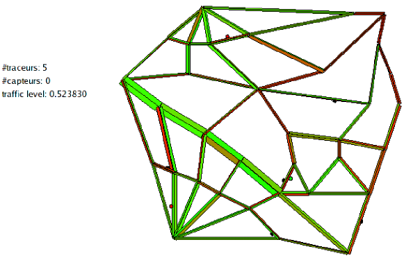
Figure 5.2: Traffic network as produced by the simulator. The continuous color code represents the traffic index from 0 (full green) to 1 (full red).

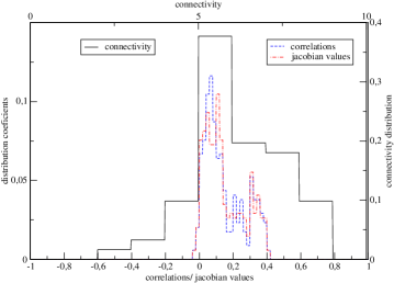
Figure 5.3: Connectivity (black), correlation coefficients (red) and Jacobian coefficients (blue) histograms for low (top) and high (bottom) noise level.

nodes	links	time steps	graph size	$\epsilon_{c_{1}}$(oscillating)	$\epsilon_{c_{2}}$ (noisy)
35	122	43	5246	0.67	1.29

Table 5.1: Toy model characteristics

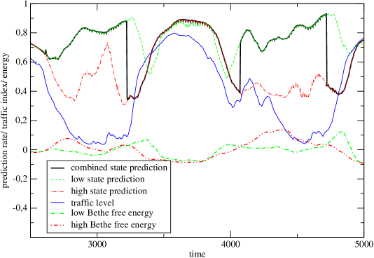
Figure 5.4: Reconstruction rates for the various possible inference states as a function of time with corresponding free energies, with $10$ probe vehicles and $\epsilon=0.75$.

Figure 5.5: Distribution of reconstruction errors for the various possible inference states for $\epsilon=0.75$.

We have tested the algorithm on the toy traffic network shown on the program’s screen-shot of Figure 5.2. The characteristics of this network are summarized in Table 5.1. Two types of traffic conditions have been used, that both correspond to periodic oscillation superimposed with noise (see blue curve of Figure 5.5); they simply differ by the level of the noise.

The two values of $\epsilon_{c}$ in Table 5.1 that have been computed for the two different traffic regimes using (4.13) are close to the observed values, which indicates that the space-time graph on which BP is run is close to the conditions of a dilute graph (Bethe lattice).

The simulation run of Figure 5.5 compares the policies of using only the low state (green), the high state (red) or the combined state w.r.t. the free energy in the low-noise case. Abrupt changes of the combined state prediction correspond to the crossing of the Bethe free energies. In the transition regimes, which correspond to out-of-equilibrium situations, the free energy criteria sometimes select the wrong state. The reason for this is that the present design of our algorithm encodes only statistical information at equilibrium. Time correlations should be incorporated in some way, to encode transition rates between the macro-states (here the low and high traffic density).

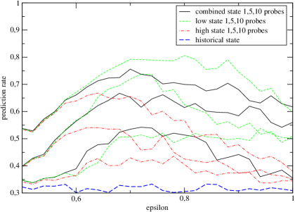
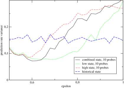
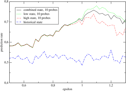
(a) (b) (c)

Figure 5.6: (a) Reconstruction rates obtained with $0$, $1$, $5$ and $10$ probe vehicles and various possible inference states; (b) variance of the reconstruction rate obtained with $10$ vehicles also for the various possible states; (c) reconstruction rates obtained for the noisy network, again with $10$ probes.

Distributions of performance errors shown in Figure 5.5 are based on a simulation run of $10000$ traffic time units where a belief propagation is run every 3 units of time for both low and high inference states, to reconstruct the traffic. Varying the parameters (either $\epsilon$ or the number of probe vehicles) and integrating the distributions up to $0.2$ yields curves of Figures 5.6 and 5.7.

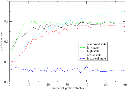
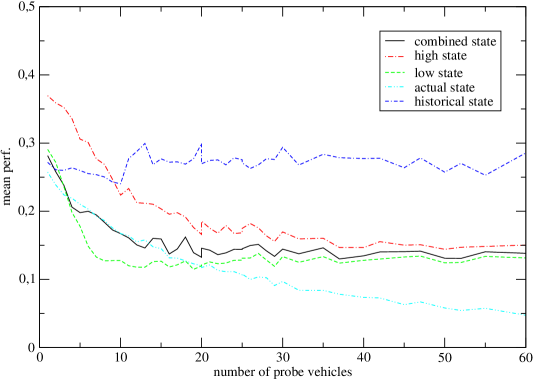
(a) (b)

Figure 5.7: (a) reconstruction rates with various possible inference states when the number of probe vehicles is varied; (b) corresponding average prediction error.

They indicate that the optimal value of $\epsilon$ for traffic prediction is slightly above the critical value for the traffic oscillating network and below the critical value for the noisy network, as expected. The fact that the prediction rate saturates at $0.8$ when the number of probe vehicles is increased in Figure 5.7 is again due to the traffic transition regimes.

6 Conclusion and perspectives

We have presented a novel methodology for reconstruction and prediction of traffic using the Belief Propagation algorithm on Floating Car Data. We have shown how the underlying Ising model can be determined in a straightforward manner and that it is unique up to some change of variables. In addition, the effect of message normalization and the stability properties can be asserted from the original data. The unfortunate fact that the BP fixed point corresponding to the historical data may be unstable can be circumvented by rescaling of the correlations. The algorithm has been implemented and illustrated using a toy traffic model.

Several generalizations are considered for future work:

• firstly, the binary description corresponding to the underlying Ising model is arbitrary. Traffic patterns could be represented in terms of $p$ different inference states. A Potts model with $p$-states variables would leave the belief propagation algorithm and its stability properties structurally unchanged. Actually this number $p$ should be subject to an optimization procedure.

• secondly, our way of encoding traffic network information might need to be augmented to cope with real world situations. This would simply amount to redefine the factor-graph used to propagate this information. In particular it is likely that a great deal of information is contained in the correlations of local congestion with aggregate traffic indexes, corresponding to sub-regions of the traffic network. Taking these correlations into account would result in the introduction of specific variables and function nodes associated to these aggregate traffic indexes. These aggregate variables would naturally lead to a hierarchical representation of the factor graph, which is necessary for inferring the traffic on large scale network. Additionally, time dependent correlations which are needed for the description of traffic, which by essence is an out of equilibrium phenomenon, could be conveniently encoded in these traffic index variables.

Ultimately, for the elaboration of a powerful prediction system, the structure of the information content of a traffic-road network has to be elucidated through a specific statistical analysis. The use of probe vehicles, based on modern communications devices, combined with a belief propagation approach, is in this respect a very promising approach.

References

- [1] T. Benz et al., Information supply for intelligent routing services – the INVENT traffic network equalizer approach, Proceedings of the ITS World Congress, 2003.
- [2] C. Berge, Théorie des graphes et ses applications, 2ème ed., Collection Universitaire des Mathématiques, vol. II, Dunod, 1967.
- [3] H. A. Bethe, Statistical theory of superlattices, Proc. Roy. Soc. London A (1935), 552.
- [4] J. Essen and M. Schreckenberg, Microscopic simulation of urban traffic based on cellular automata, Int. J. Mod. Phys. (1997), C8:1025–1036.
- [5] C. Furtlehner, A. de La Fortelle, and J.-M. Lasgouttes, Belief-propagation algorithm for a traffic prediction system based on probe vehicles, Tech. Report 5807, Inria, 2006.
- [6] F. Harary, The determinant of the adjacency matrix of a graph, Siam Review Vol. 4 (1962), no. No. 3, pp. 202–210.
- [7] T. Heskes, On the uniqueness of loopy belief propagation fixed points, Neural Computation 16 (2004), 2379–2413.
- [8] E. Ising, Beitrag zur Theorie des Ferromagnetismus, Zeitschr. f. Phys. 31 (1925), 253–258.
- [9] J. M. Mooij and H. J. Kappen, On the properties of the Bethe approximation and loopy belief propagation on binary network, J. Stat. Mech. (2005), P11012.
- [10] M. Mézard, G. Parisi, and M.A. Virasoro, Spin glass theory and beyond, World Scientific, Singapore, 1987.
- [11] K. Nagel and M. Schreckenberg, A cellular automaton model for freeway traffic, J. Phys. I,2 (1992), 2221–2229.
- [12] J. Pearl, Probabilistic reasoning in intelligent systems: Network of plausible inference, Morgan Kaufmann, 1988.
- [13] PRIME project, Technology assessment and expected targets, Deliverable D3.2, 2000.
- [14] H. H. Versteegt and C. M. J. Tampère, PredicTime - state of the art and functional architecture, Tech. Report 2003-07, TNO Inro, 2003.
- [15] J. S. Yedidia, W. T. Freeman, and Y. Weiss, Generalized belief propagation, Advances in Neural Information Processing Systems (2001), 689–695.
- [16] , Constructing free-energy approximations and generalized belief propagation algorithms, IEEE Trans. Inform. Theory. 51 (2005), no. 7, 2282–2312.