Universal statistical properties of poker tournaments

Abstract

We present a simple model of Texas hold’em poker tournaments which retains the two main aspects of the game: i. the minimal bet grows exponentially with time; ii. players have a finite probability to bet all their money. The distribution of the fortunes of players not yet eliminated is found to be independent of time during most of the tournament, and reproduces accurately data obtained from Internet tournaments and world championship events. This model also makes the connection between poker and the persistence problem widely studied in physics, as well as some recent physical models of biological evolution, and extreme value statistics.

I Introduction

Physicists are now more then ever involved in the study of complex systems which do not belong to the traditional realm of their science. Finance (options theory,…) bouchaud , human networks (Internet, airports,…) barabasi , the dynamics of biological evolution krug ; leadcs and in general of competitive “agents” krap ; red1 ; red2 are just a few examples of problems recently addressed by statistical physicists. However, many of these systems are not isolated and are thus sometimes very difficult to describe quantitatively: a financial model cannot predict the occurrence of wars or natural disasters which certainly affect financial markets, nor can it include the effect of all important external parameters (China’s GDP growth, German exports, Google’s profit…). Rather, these studies try to capture important qualitative features which, interestingly, are sometimes universal. In this context, universality means that large scale aspects of the real system are properly reproduced by a simple model which only retains the main relevant ingredients of the original physics. Adding further details to the model does not affect these universal properties.

In the present work, we study a very human and playful activity: poker tournaments. Although a priori governed by human laws (bluff, prudence, aggressiveness…), we shall find that some of their interesting properties can be quantitatively described. One of the appealing aspects of a poker tournament lies in the obvious fact that it is a truly isolated system, which is not affected by any external phenomenon. Two famous mathematicians (Émile Borel borel , and later John von Neumann neumann ) contributed to the science of poker. However, they concentrated on head-to-head games, like their most recent followers ferg , obtaining the best strategy in terms of the value of the hand and the pot. To our knowledge, the present work represents the first study of large scale poker tournaments. Note however that in a recent work red1 , the authors study head-to-head elimination tournaments involving seeded competitors, and apply successfully their theory to the US college basketball national championship.

In the following, we introduce a simple model which can be treated analytically and which faithfully reproduces some properties of Internet and live poker tournaments. Our main quantities of interest are the distribution of the fortunes of surviving players, their decay rate, the number of different players owning the biggest fortune at any given time during the tournament (dubbed the “chip leader”), and the distribution of their fortune. Interestingly, the constraint that a surviving player must keep a positive fortune relates poker tournaments to the problem of persistence AB1 ; per1 ; SM , and the competitive nature of the game connects some of our results with recent models of competing agents krug ; leadcs ; krap ; red1 ; red2 . In addition, the properties of the chip leader display extreme value statistics, a phenomenon observed in many physical systems red1 ; extreme ; gumbel .

In Section II, we define a stochastic model which retains the main identified ingredients of poker tournaments: i. the minimal bet grows exponentially with time; ii. players have a finite probability $q$ to bet all their money. In Section III, we first solve the corresponding model for $q=0$, which will allow us to make the connection with the persistence problem widely studied by physicists. In Section IV, we will show that $q$ must physically take a specific value, and thus is not a free parameter. The results of the model will compare favorably with actual data recorded from real Internet poker tournaments and World Poker Tour main events. Finally, in the last Section V, we will consider the statistical properties of the chip leader. In particular, we will show the connection with the “leader problem” arising in evolutionary biophysics, and the field of extreme value statistics which has recently attracted a lot of attention from physicists.

II A simple poker model

Before addressing the basic rules of poker and the resulting definition of our model, we wish to introduce some useful poker terminology. In a real poker tournament, players first pay the same entry fee or “buy-in” (from 1 $ to 25000 $) which is converted in “chips”. Hence players are not betting actual money but chips. The total number of chips of a player is called his “stack”. At any time in the tournament, if a player decides to bet his entire stack, it is said that he is going “all-in”.

We now describe the main aspects of a Texas hold’em poker tournament, currently the most popular form of poker. Initially, $N_{0}$ players sit around tables accepting up to $\theta=10$ players. In real poker tournaments, $N_{0}$ typically lies in the range $N_{0}\sim 10-10000$. We do not detail the precise rules of Texas hold’em poker, as we shall see that their actual form is totally irrelevant provided that two crucial ingredients of the game are kept:

$\bullet$ A tournament consists in a series of independent games or “deals”. Before a deal starts, the two players next to the dealer (i.e. the player dealing the cards) post the minimal bet, which is called the “blind”. This term arises from the fact that they bet before actually seeing their cards. The blinds also ensure that there is some money in the pot to play for at the very start of the game. The blind $b$ increases exponentially with time, and typically changes to the value 40 $, 60 $, 100 $, 200 $, 300 $, 400 $,… every 10-15 minutes on Internet tournaments, hence being multiplied by a factor 10 every hour or so. We shall see that the growth rate of the blind entirely controls the pace of a tournament, a phenomenon observed in another context in red2 . Therefore, the fact that the blind grows exponentially with time must be a major ingredient of any realistic model of poker.

$\bullet$ The next players post their bets ($\geq b$) according to their evaluation of the two cards they each receive. There are subsequent rounds of betting following the successive draws of five common cards. Ultimately, the betting player with the best hand of five cards (selected from its two cards and the five common cards) wins the pot. Most of the deals end up with a player winning a small multiple of the blind. However, during certain deals, two or more players can aggressively raise each other, so that they finally bet a large fraction, if not all, of their chips. This can happen when a player goes all-in, hence betting all his chips. Any serious model of poker should take into account the fact that players often bet a few blinds, but sometimes end up betting all or a large fraction of their chips.

Once a player loses all his chips, he is eliminated. During the course of the tournament, some players may be redistributed to other tables, in order to keep the number of tables minimum.

Retaining the two main ingredients mentioned above, we now define a simple version of poker which turns out to describe quantitatively the evolution of real poker tournaments. The $N_{0}$ initial players are distributed at tables with $\theta=10$ seats. They receive the same amount of chips $x_{0}\gg b_{0}$, where $b_{0}$ is the initial blind. The ratio $x_{0}/b_{0}$ is typically in the range $50-100$ in actual poker tournaments.

$\bullet$ The players take turns at dealing. In the model, only the player next to the dealer, dubbed the “blinder”, posts the blind bet. The blind increases exponentially with time as, $b(t)=b_{0}\exp(t/t_{0})$.

$\bullet$ The tables run in parallel. At each table, the players receive one card, $c$, which is a random number uniformly distributed between 0 and 1.

$\bullet$ We define a critical hand value $c_{0}\in[0,1]$. The following players bet the value $b$ with probability $e(c)$, if $0\leq c\leq c_{0}$. $e(c)$ is an evaluation function, whose details will be immaterial. Intuitively, $e(c)$ should be an increasing function of $c$, implying that a player will more often play good hands than bad ones. We tried several forms of $e(c)$, obtaining the same results. In our simulations, we choose $e(c)=c^{n}$, where $n$ is the number of players having already bet, including the blinder. In this case, $e(c)$ is simply the probability that $c$ is the best card among $n+1$ random cards. This reflects the fact that a player should be careful when playing bad hands if many players have already bet. Determining the optimal evaluation function for a given $\theta$, in the spirit of Borel’s and von Neumann’s analysis for $\theta=2$, is a formidable task which is left for a future study csnext .

$\bullet$ The first player with a card $c>c_{0}$ goes all-in, so that $q=1-c_{0}$ is the probability to go all-in. The next players including the blinder can follow if their card is greater than $c_{0}$, and fold otherwise. If a player with a card $c>c_{0}$ cannot match the amount of chips of the first player all-in, he simply bets all his chips, but can only expect to win this amount from each of the other players going all-in.

$\bullet$ Finally, the betting player with the highest card wins the pot and the blinder gets the blind back if nobody else bets. The players left with no chips are eliminated, and after each deal, certain players may be redistributed to other tables, in a process ensuring that the number of tables remains minimum at all times and that no table has less than $[N/\theta]$ players, where $[\bf{\cdot}]$ denotes the integer part function. After a deal is completed at all tables, time is updated to $t+1$, and the next deal starts. This process is repeated until only one player is left.

III Poker model without all-in processes

Let us first consider the unrealistic case $q=0$. The amount of chips or stack $x(t)$ of a given player evolves according to $x(t+1)=x(t)+\varepsilon(t)b(t)$. The effective noise $\varepsilon(t)$ should have zero average since all players are considered equal and there is therefore no individual winning strategy in the mathematical sense. $\varepsilon(t)$ is also Markovian, since successive deals are uncorrelated. We define $\bar{x}(t)$ as the statistical average of $x(t)$. If the typical value of $x\sim\bar{x}(t)$ remains significantly bigger than the blind $b(t)$, we can adopt a continuous time approach. Hence, the evolution of $x(t)$ is that of a generalized Brownian walker:

$$\frac{dx}{dt}=\sigma b(t)\eta(t),$$ (1)

where $\sigma^{2}=\bar{\varepsilon^{2}}$ is a constant of order unity, and $\eta(t)$ is a $\delta$-correlated white noise. The number of surviving players with $x$ chips, $P(x,t)$, evolves according to the Fokker-Planck equation

$$\frac{\partial P}{\partial t}=\frac{\sigma^{2}b^{2}(t)}{2}\frac{\partial^{2}P}{\partial x^{2}},$$ (2)

with the absorbing boundary condition $P(x=0,t)=0$, and initial condition $P(x,t=0)=\delta(x-x_{0})$. This kind of problem arises naturally in physics in the context of persistence, which is the probability that a random process $x(t)$ never falls below a certain level AB1 ; per1 ; SM . Defining

$$\tau(t)=\frac{\sigma^{2}b_{0}^{2}t_{0}}{2}\left({\rm e}^{\frac{2t}{t_{0}}}-1\right),$$ (3)

Eq. (2) can be solved by the method of images per1 :

$$P(x,t)=\frac{N_{0}}{\sqrt{2\pi\tau(t)}}\left({\rm e}^{-\frac{(x-x_{0})^{2}}{2\tau(t)}}-{\rm e}^{-\frac{(x+x_{0})^{2}}{2\tau(t)}}\right).$$ (4)

Note that the above result holds for any form of $b(t)$, provided that one properly defines $\tau(t)=\sigma^{2}\int_{0}^{t}b^{2}(t^{\prime})\,dt^{\prime}$.

For large time (or $\tau\gg 1$), the distribution of chips becomes scale invariant

$$P(x,t)=\frac{N(t)}{\bar{x}(t)}f\left(\frac{x}{\bar{x}(t)}\right),$$ (5)

where the density of surviving players is given by

$$\frac{N(t)}{N_{0}}=\frac{2x_{0}}{\sqrt{\pi t_{0}}\sigma b_{0}}{\rm e}^{-\frac{t}{t_{0}}}.$$ (6)

We find that the decay rate of the number of players is exactly given by the growth rate of the blind, which thus controls the pace of the tournament. The total duration of a tournament $t_{\rm f}$ is typically

$$\frac{t_{\rm f}}{t_{0}}=\ln(N_{0})-\frac{1}{2}\ln(t_{0})+\ln\left(\frac{x_{0}}{b_{0}}\right),$$ (7)

which only grows logarithmically with the number of players and the ratio ${x_{0}}/{b_{0}}$. The average stack is proportional to the blind

$${\bar{x}(t)}=\frac{N_{0}}{N(t)}x_{0}=\frac{\sqrt{\pi t_{0}}\sigma}{2}b(t).$$ (8)

When $t_{0}\gg 1$, this expression implies that ${\bar{x}(t)}/b(t)\gg 1$, hence validating the use of a continuous time approach. Finally, we find that the normalized distribution of chips is given by the Wigner distribution

$$f(X)=\frac{\pi}{2}X{\rm e}^{-\frac{\pi}{4}X^{2}},\quad F(X)=1-{\rm e}^{-\frac{\pi}{4}X^{2}},$$ (9)

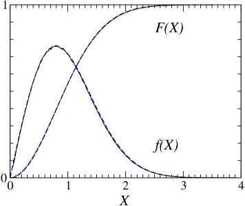
Figure 1: We plot the normalized distribution of chips $f(X)$ and its cumulative sum $F(X)$ obtained from numerical simulations of our poker model with $q=0$ (thin lines; $N_{0}=10000$, $t_{0}=2000$, $x_{0}/b_{0}=100$, $10000$ “tournaments” played). These distributions are extracted at times for which $N(t)/N_{0}=50$%, 30%, 10%. The dashed lines correspond to the exact solution, Eq. (9).

where $F(X)=\int_{0}^{X}f(Y)\,dY$. Equivalently, in the context of persistence, $f$ is naturally found to be the first excited eigenstate of the quantum harmonic oscillator per1 . The scaling function $f$ is universal, i.e. independent of all the microscopic parameters ($b_{0}$, $t_{0}$, $x_{0}$…). In Fig. 1, we plot the normalized distribution $f(X)=\bar{x}(t)P(x,t)/N(t)$ and its cumulative sum $F(X)$ as a function of $X=x/\bar{x}(t)$, as obtained from extensive numerical simulations of the present poker model with $q=0$. We find a perfect data collapse on the analytical result of Eq. (9).

IV Poker model including all-in processes

Let us now consider the more realistic case $q>0$ (or $c_{0}<1$). A priori, it seems that $q$ is a new parameter whose precise value could dramatically affect the dynamics of the game. In reality, $q$ must be intimately related to the decay rate $t_{0}^{-1}$ of the number of players, which is imposed by the exponential growth of the blind. To see this, let us first compute the decay rate due to the all-in processes. At a given table, and for small $q$, the probability that an all-in process occurs is given by

$$P_{\rm all-in}=\frac{q^{2}\theta(\theta-1)}{2},$$ (10)

where the factor $q^{2}$ is the probability that two players go all-in, and ${\theta(\theta-1)}/{2}$ is the number of such pairs. Expecting $q\ll 1$, we have neglected all-in processes involving more than two players. During a two-player all-in process, there is a probability $1/2$ that the losing player is the one with the smallest number of chips (he is then eliminated). Cumulating the results of the $N/\theta$ tables, we find the density decay rate due to all-in processes

$$\frac{dN}{dt}_{\rm all-in} = -\frac{1}{2}{\times}\frac{N}{\theta}{\times}P_{\rm all-in}=-\frac{N}{t_{\rm all-in}},$$ (11)

$$t_{\rm all-in} = \frac{4}{q^{2}(\theta-1)}.$$ (12)

We now make the claim that the physically optimal choice for $t_{\rm all-in}$, and hence for $q$, is such that the decay rate due to all-in processes is equal to the one caused by the stack fluctuations of order $b(t)$. Since the total decay rate will be shown to remain equal to $t_{0}^{-1}$, $t_{\rm all-in}=2t_{0}$ should hold, since inverse decay rates add up. If $t_{\rm all-in}<2t_{0}$, the game is dominated by all-in processes and $x(t)$ can get rapidly large compared to $b(t)$. The first player to go all-in is acting foolishly and takes the risk of being eliminated just to win the negligible blind. Inversely, if $t_{\rm all-in}>2t_{0}$, players (especially those with a declining stack) would be foolish not to make the most of the opportunity to double their chips by going all-in. We expect that real poker players would, on average, self-adjust their $q$ to its optimal value. Finally, we find that $q$ is not a free parameter, but should take the physical value

$$q=\sqrt{\frac{2}{(\theta-1)t_{0}}}.$$ (13)

We now write the exact evolution equation for the number of surviving players with $x$ chips, combining the effect of pots of order $b$ and all-in processes

$$\frac{\partial P}{\partial t}=\frac{\sigma^{2}b^{2}}{2}\frac{\partial^{2}P}{\partial x^{2}}+\frac{2}{t_{0}}(K(P)-P),$$ (14)

where the non linear all-in kernel $K$ is given by

$$K(P) = \frac{1}{4}P(x/2)\int_{x/2}^{+\infty}\frac{P(y)}{N}\,dy$$ (15)

$$+ \frac{1}{2}\int_{0}^{x/2}P(x-y)\frac{P(y)}{N}\,dy$$

$$+ \frac{1}{2}\int_{0}^{+\infty}P(x+y)\frac{P(y)}{N}\,dy,$$

and where we have dropped the time variable argument for clarity. In Eq. (14), the factor ${2}/{t_{0}}=q^{2}(\theta-1)$ is simply the rate of all-in processes involving the considered player, without presuming the outcome of the event. In addition, the first term of Eq. (15) describes processes where the considered player has doubled his chips by winning against a player with more chips than him. The second term corresponds to an all-in process where the player has won against a player with less chips than him (and has eliminated this player). Finally, the last term describes the loss against a player with less chips than him (otherwise the considered player is eliminated). Integrating Eq. (15) over $x$, we check that the probability to survive an all-in process is $\frac{3}{4}$, the two first terms adding up to $\frac{1}{2}$. Indeed, the player survives if he wins (with probability $\frac{1}{2}$) or if he loses, but only against a player with less chips (with probability $\frac{1}{4}$). We recover the decay rate associated to all-in processes, $\left(1-\frac{3}{4}\right){\times}\frac{2}{t_{0}}=t_{\rm all-in}^{-1}$.

We now look for a scaling solution of Eq. (15) of the form

$$P(x,t)=\frac{\lambda}{\hat{x}(t)^{2}}f\left(\frac{x}{\hat{x}(t)}\right),$$ (16)

where the integral of $f$ is normalized to 1, so that ${N(t)}={\lambda}/{\hat{x}(t)}$. Plugging this ansatz into Eq. (14), we find that one must have $\hat{x}(t)\sim b(t)$ for all the terms to scale in the same manner. Defining

$$\hat{x}(t)=\frac{\sqrt{t_{0}}\sigma b(t)}{2}\sim\bar{x}(t)\sim{\rm e}^{\frac{t}{t_{0}}},$$ (17)

and the scaling variable $X=x/\hat{x}(t)$, we obtain the following integrodifferential equation for $f(X)$

$$f^{\prime\prime}(X)+Xf^{\prime}(X)+\frac{1}{2}f(X/2)\int_{X/2}^{+\infty}f(Y)\,dY$$

$$+\int_{0}^{X/2}f(X-Y)f(Y)\,dY$$

$$+\frac{1}{2}\int_{0}^{+\infty}f(X+Y)f(Y)\,dY=0,$$ (18)

with the boundary condition $f(0)=0$. We did not succeed in solving this equation analytically. However, the small and large $X$ behavior of $f(X)$ can be extracted from Eq. (18):

$$f(X)\mathop{\sim}\limits_{X\to 0}\frac{X}{2},\quad\,f(X)\mathop{\sim}\limits_{X\to+\infty}2\mu{\rm{e}}^{-\mu X}.$$ (19)

Thus, when including all-in processes, the universal scaling distribution decays more slowly than for $q=0$. Eq. (18) can be easily solved numerically using a standard iteration scheme, and we find $\mu\approx 1.562$.

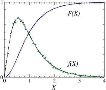
Figure 2: We plot the normalized distribution of chips $f(X)$ and its cumulative sum $F(X)$ obtained from numerical simulations of our poker model (thin dotted lines, $N_{0}=10000$, $t_{0}=2000$, $x_{0}/b_{0}=100$, $10000$ “tournaments” played). These distributions are extracted at times for which $N(t)/N_{0}=50$%, 30%, 10%. The dashed lines correspond to the numerical solution of the exact Eq. (18). The data recorded from 20 real poker tournaments (totalizing 1584 players still in) are also plotted (full lines), and are found to agree remarkably with the present theory. Note that $f(X)$ for real tournaments was obtained by differentiating a fitting function to the actual cumulative sum. We also plot the standard but noisier bin plot of the distribution of chips in real poker tournaments (circles).

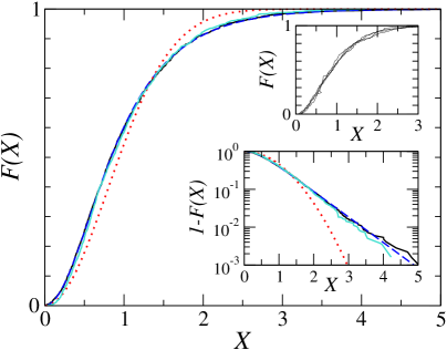
Figure 3: We plot the integrated density distribution $F(X)$ extracted from Internet tournaments (same as Fig. 2; black line), and from the four main events of the WPT 2006 season (ranking after day 1 and day 2 totalizing 1256 players; turquoise line), and compare them to the numerical solution of the exact Eq. (18) (dashed line), and to the analytical result Eq. (9) of the poker model for $q=0$ (dotted line). The bottom insert illustrates the exponential decay of $1-F(x)$, instead of the Gaussian decay predicted by the simple model with $q=0$. In the top insert, we plot $F(X)$ for each individual WPT tournaments (day 1 only; for the sake of clarity).

In Fig. 2, we plot the normalized distribution $f(X)$ as a function of $X=x/\bar{x}(t)$ obtained from extensive numerical simulations of the present poker model, with $q$ given by Eq. (13). We find a perfect data collapse on the numerical solution of the exact scaling equation Eq. (18). In order to check the relevance of this parameter-free distribution to real poker tournaments, we visited two popular on-line poker playing zones, and followed 20 no-limit Texas hold’em tournaments with an initial number of players in the range $250-800$. When the number of players was down to the range $N\sim 60-130$, we manually recorded their number of chips disclaim . Fig. 2 shows the remarkable agreement between these data and the results of the present model. The maximum of the distribution corresponds to players holding around 55% of the average number of chips per player. In addition, a player owning twice the average stack per player $(X=2)$ precedes 90% of the other players, whereas a player with half the average stack $(X=1/2)$ precedes only 25% of the other players. In Fig. 3, we compare these results to data collected from the four main events of the World Poker Tour 2006 season wpt . Although the level of play is incomparably better than on typical Internet poker rooms (the buy-in of 10000 $ or more is also incomparable), the stacks distributions are very similar and decay exponentially (see the prediction of Eq. (19)), as illustrated in the bottom insert of Fig. 3. The model without all-in events ($q=0$) would predict a faster Gaussian decay. The fact that we find similar results for two very different kinds of poker tournaments certainly justifies the universal nature of the present theory.

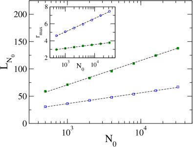
Figure 4: We plot the average number of chip leaders $L_{N_{0}}$ as a function of the number of initial players $N_{0}$, finding a convincing logarithmic growth (full symbols correspond to the case $q=0$). The insert shows the logarithmic growth of $r_{\rm max}$ (defined in the text). The dashed lines correspond to log-linear fits of the data.

V Properties of the chip leader

We now consider the statistical properties of the player with the largest amount of chips at a given time, dubbed the chip leader. First, we consider the average number of chip leaders $L_{N_{0}}$ in a tournament with $N_{0}$ initial players. In many competitive situations krug ; leadcs ; krap , arising for instance in biological evolution models krug ; leadcs , it is found that $L_{N_{0}}$ grows logarithmically with the number of competing agents $N_{0}$, a general result which has been established analytically in leadcs .

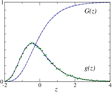
Figure 5: We plot the normalized cumulative distribution $G(z)$ of the fortune of the chip leader recorded when $N(t)/N_{0}=40$%, 20%, 10% (thin dotted lines, all-in processes included, $N_{0}=10000$, $t_{0}=2000$, $x_{0}/b_{0}=100$, $10000$ “tournaments” played). We also plot the derivative $g(z)$ of a multi-variable fit of these data (full line) as well as the standard scatter bin plot (circles). The data convincingly follow the universal Gumbel distribution (dashed lines).

We confirm that in the present model, with or without all-in processes, the same phenomenon is observed (see Fig. 4). We have also computed the average maximum ratio $r_{\rm max}={\sup_{t}\bar{x}_{\rm lead}/\bar{x}}$. In the present model, $x_{\rm lead}/\bar{x}$ increases rapidly on a scale of order $t_{0}$, and then decays (almost linearly with time) to $\sim 1.5$, where it becomes non self-averaging due to large fluctuations at the end of the tournament. Fig. 4 illustrates the logarithmic growth of $r_{\rm max}$ as a function of $N_{0}$. For $N_{0}=500$, which is typical of Internet tournaments, we find $r_{\rm max}\approx 4.6$, which is fully compatible with a superficial analysis of real data.

Extreme value statistics have recently attracted a lot of attention from physicists in various contexts extreme . In this regard, we have checked that $z=(x_{\rm lead}-\bar{x}_{\rm lead})/({\bar{x^{2}}_{\rm lead}-\bar{x}^{2}_{\rm lead}})^{1/2}$ is distributed according to the universal Gumbel distribution

$$g(z)=\frac{\pi}{\sqrt{6}}\exp[-Z-\exp(-Z)],$$ (20)

where $Z=\pi z/\sqrt{6}+\gamma$, and $\gamma$ is Euler’s constant. Such a behavior, which is typical of independent, or at least weakly correlated random variables gumbel , is illustrated on Fig. 5.

VI Conclusion

In this paper, we have developed a quantitative theory of poker tournaments and made the connection between this problem and persistence in physics, the leader problem in evolutionary biology, and extreme value statistics. In particular, we have identified the two main ingredients controlling the dynamics of a tournament: the exponential increase of the blind, and the necessity to include all-in events where at least two players bet their entire stack. In order to mimic the play of “intelligent” players, we found that the probability of going all-in should take a well-defined value. This theory leads to a quantitative understanding of the scale-invariant stack distribution observed in Internet and WPT tournaments, and predicts rich statistical features concerning the chip leader.

In a future work csnext , we plan to implement in our model the optimal strategies for folding, betting or going all-in, hence eliminating the only free parameter $q$. Preliminary results csnext indicate that the optimal probability $q_{0}$ to be the first to go all-in is a simple function of the current pot $P$, of the chip stack $x$ of the considered player, and of $x_{k}$, the stack of the $k$-th player left to bet (among a total of $n$ such players). Defining $X_{k}=\min(x_{k},x)$, and $q_{k}$ as the probability that the player $k$ calls the all-in bet of the first player (and neglecting multiple calls), we find csnext

$$q_{k} = q_{0}\frac{X_{k}+P}{X_{k}+2P},$$ (21)

$$P = \sum_{k=1}^{n}q_{k}X_{k}\prod_{j=k}^{n}\left(1-q_{j}\right)^{-1},$$ (22)

where $q_{0}$ is the solution of the implicit Eq. (22), after inserting the expression of $q_{k}$ obtained in Eq. (21). A detailed analysis of Eqs. (21,22) reveals that the obtained optimal strategy perfectly reproduces qualitative features observed in real tournaments, notably the fact that players with a small stack go more often all-in than others (and are often called). In addition, direct confrontations between two players owning a big stack (in units of $\bar{x}$) are rare, except if the pot is already huge, and only happens when both players have a very good hand.

Finally, it would be interesting to obtain access to the full dynamical evolution of a large sample of real-life poker tournaments, in order to check the predictions of the model concerning the chip leader and to identify other remarkable statistical properties of poker tournaments.

- (1) J.-P. Bouchaud and M. Potters, Theory of financial risk and derivative pricing: from statistical physics to risk management, Cambridge University Press (2003).
- (2) A.-L. Barabási and R. Albert, Rev. Mod. Phys. 74, 47 (2002); M. Newman, A.-L. Barabási, and D. J. Watts, The structure and dynamics of networks, Princeton University Press (2006).
- (3) J. Krug and C. Karl, Physica A 318, 137 (2003); K. Jain and J. Krug, J. Stat. Mech., P04008 (2005).
- (4) C. Sire, S. N. Majumdar, and D. S. Dean, J. Stat. Mech., L07001 (2006).
- (5) P. L. Krapivsky and S. Redner, Phys. Rev. Lett. 89, 258703 (2002); E. Ben-Naim and P. L. Krapivsky, Euro. Phys. Lett. 65, 151 (2004).
- (6) E. Ben-Naim, S. Redner, and F. Vazquez, Europhys. Lett. 77, 30005 (2007).
- (7) E. Ben-Naim and S. Redner, J. Phys. A 37, 11321 (2004).
- (8) E. Borel, Traité du calcul des probabilités et ses applications, Vol. IV, Gautier-Villars (Paris, 1938); note that Émile Borel’s book on probability in the game of bridge has been recently reprinted by Eds. Jacques Gabay (Paris).
- (9) J. von Neumann and O. Morgenstern, The theory of games and economic behavior, Princeton University Press (1944).
- (10) C. Ferguson and T. S. Ferguson, Game Theory and Applications, Nova Sci. Publ. 9, 17 (New York, 2003).
- (11) A. J. Bray, B. Derrida, and C. Godrèche, J. Phys. A 27, L357 (1994); B. Derrida, V. Hakim, and V. Pasquier, Phys. Rev. Lett. 75, 751 (1995).
- (12) S. N. Majumdar and C. Sire, Phys. Rev. Lett. 77, 1420 (1996), K. Oerding, S. J. Cornell, and A. J. Bray, Phys. Rev. E 56, R25 (1997).
- (13) S. N. Majumdar, Current Science 77, 370 (1999).
- (14) A. Comtet, P. Leboeuf, and S. N. Majumdar, Phys. Rev. Lett. 98, 070404 (2007); D.-S. Lee, Phys. Rev. Lett. 95, 150601 (2005); C. J. Bolech and A. Rosso, Phys. Rev. Lett. 93, 125701 (2004).
- (15) E. J. Gumbel, Statistics of extremes, Columbia University Press (1958).
- (16) C. Sire, unpublished. For instance, in the case and , the optimal strategy of the player next to the blinder consists in betting if and to fold otherwise. The last player bets if and the preceding player has folded, and bets if and the preceding player has bet. Note that the blinder has a positive expectancy to lose money.
- (17) Internet tournament data have been collected on the poker playing zones Poker Stars (www.pokerstars.com) and PartyPoker (www.partypoker.com).
- (18) WPT tournaments results have been obtained from www.pokerpages.com/tournament.