Towards a physics of evolution: Existence of gales of creative deconstruction in evolving technological networks

Abstract

Systems evolving according to the standard concept of biological or technological evolution are often described by catalytic evolution equations. We study the structure of these equations and find a deep relationship to classical thermodynamics. In particular we can demonstrate the existence of several distinct phases of evolutionary dynamics: a phase of fast growing diversity, one of stationary, finite diversity, and one of rapidly decaying diversity. While the first two phases have been subject to previous work, here we focus on the destructive aspects – in particular the phase diagram – of evolutionary dynamics. We further propose a dynamical model of diversity which captures spontaneous creation and destruction processes fully respecting the phase diagrams of evolutionary systems. The emergent timeseries show a Zipf law in the diversity dynamics, which is e.g. observable in actual economical data, e.g. in firm bankruptcy data. We believe the present model is a way to cast the famous qualitative picture of Schumpeterian economic evolution, into a quantifiable and testable framework.

I Introduction

Simplistically technological evolution is a process of (re)combination and substitution of existing elements to invent and produce new goods, products or things. New things can come into existence through combining existing ones in whole or part. The new things then undergo a ’valuation’ (selection) process based on their ’utility’ associated to them in the context of their surroundings. The surroundings are defined by all other yet existing things, and all things which may come into existence in the foreseeable future. Another way how new things can come to being is pure chance, such as random inventions which do not rely on pre-existing things. Biological evolution is a special case of technological evolution (i.e. innovation), where recombination and substitution happens through sexual reproduction and mutations.

The dynamics of systems capable of evolution have been formalized some time ago. In this context the concept of the adjacent possible has been brought forward origin . The adjacent possible is the set of objects that can get produced within a given time span into the future. What can get produced in the next timestep depends crucially on the details of the set of elements that exist now. To capture the dynamics of an evolving system which is governed by a combination/substitution mechanism, imagine that the diversity of the system is given by a $d$ dimensional state vector $x$. Each element $x_{i}$ characterizes the abundance of all possible elements $i$. This means that the total number of all elements that can potentially ever exist in the system are bounded from above by $d$ . Its dynamics is governed by the famous equation

$$\frac{\partial}{\partial t}x_{i}=\alpha_{ijk}x_{j}x_{k}-x_{i}\sum_{l}\alpha_{ljk}x_{j}x_{k}\quad,$$ (1)

where the second term ensures normalization of $x$. $x$ thus captures the relative abundances of existing elements. The tensor elements $\alpha_{ijk}$ serve as a ’rule table’, telling which combination of two elements $j$ and $k$ can produce a third (new) element $i$. The element $\alpha_{ijk}$ is the rate at which element $i$ can get produced, given the elements $j$ and $k$ are abundant at their respective concentrations $x_{j}$ and $x_{k}$. Equation (1) has a long tradition; some of its special cases are the Lotka Volterra replicators see e.g. in lotka , the hypercycle hyper , or the Turing gas turing . Equation (1) has been analyzed numerically farmer1 ; numerical , however system sizes are extremely limited. In contrast to the amount of available qualitative and historical knowledge on evolution gould , surprisingly little effort has been undertaken to solve Eq. (1) explicitly. To understand the dynamics of Eq. (1) more deeply and analytically it was suggested in hanel05 to assume three things: (i) the focus is shifted from the actual concentration of elements $x_{i}$, to the system’s diversity. Diversity is defined as the number of existing elements. An element exists, if $x_{i}>0$, and does not exist if $x_{i}=0$. (ii) For simplicity, the rule table $\alpha$ is assumed to have binary entries, $0$ and $1$ only, (iii) the location of the non-zero entries is perfectly random. To characterize the number of these entries the number $r$ is introduced, which is the rule table density or the density of productive pairs. The total number of productive pairs in the system (i.e. the number of non-zero entries in $\alpha$) is consequently given by $r\,d$.

With these assumptions, the idea in hanel05 was to explicitly formalize the concept of the adjacent possible, so that Eq. (1) could be rewritten into a dynamical map whose asymptotic limit could be found analytically. The only variable of the corresponding map is $r$. The initial condition, i.e., the initial size of present elements is assigned $a_{0}$. The solution of the system is the asymptotical value ($t\to\infty$) of diversity, $a_{\infty}$. The amazing result of this solution, (as a function of $r$ and the initial condition $a_{0}$) is that evolutionary systems of the type of Eq. (1) have a phase transition in the $r$-$a_{0}$ plane. In one of the two phases – after a few iterations – no more elements can be built up from existing ones and the total diversity converges to a finite number (sub-critical phase). The other phase is characterized that the advent of new elements creates so many more possibilities to create yet other elements that the system ends up producing all or almost all possible $d$ elements This we call the super-critical or ’fully populated’ phase. Even though the existence of a phase transition was hypothesized some time ago in origin , it is entirely surprising that the phase transition is mathematically of exactly the same type as a Van der Waals gas . Note that this model is a mathematically tractable variant of the so called bit-string model of biological evolution, introduced in origin .

The dynamics discussed so far assumes that a system is starting with relatively low diversity $a_{0}$, which increases over time, up to a final asymptotic level, $a_{\infty}$. However, also the opposite dynamics is possible. Imagine one existing element, say $i$, is removed from the system, a species is dying out, or a technical tool gets out of fashion/production. This removal can imply that other elements, which needed $i$ as a production input will also cease to exist, unless some other way exists to produce them (not involving $i$). Note, that all the necessary information is incorporated in $\alpha$.

The first part of this paper studies the dynamics of evolutionary systems which exist in the highly populated phase, and where $\delta_{0}$ elements get kicked out at the initial timestep. These defected elements may trigger others to default as well. We demonstrate the existence of a new phase transition in the $\delta_{0}$-$r$ plane, meaning that for a fixed rule density $r$ there exists a critical value of initial defects, above which the majority of elements will die out in a cascade of secondary defects.

The understanding of these phase diagrams teaches something about the class of dynamical systems to which the mechanism of evolution belongs to. However, this is only part of the story: it does not yet constitute the (microscopic) dynamics of the system .

In reality, the final diversity $a_{\infty}$ will not be a constant, but will be subject to fluctuations. The relevant parameter will become the diversity (number of nonzero elements in $x$) over time, $a_{t}$. In particular, there are two types of fluctuations: elements will get created spontaneously with a given rate, and existing elements will go extinct with another rate. The second part of this work proposes a dynamical model of an evolutionary system incorporating these spontaneous processes, compatible with their inherent phase diagrams. The model is characterized by the rule density $r$, one creation and one destruction process, the latter ones modeled by simple Poisson processes. We study the resulting dynamics and find several characteristics typical to critical systems and destructive economical dynamics described qualitatively by J. A. Schumpeter a long time ago schumpeter11 .

II The creative phase transition

The dynamics of diversity (number of existing elements over time) has been analytically solved in hanel05 . To be self-consistent in this section we review the argument: It is first assumed that the system has a growing mode only (tensor elements $\alpha_{ijk}$ are zero or one but never negative). For this situation Eq. (1) was projected onto a dynamical map, whose asymptotic solutions can be found.

If the number of non-zero elements in $x(t)$ is denoted by $a_{t}$, it was shown in hanel05 that the non-linear, second order recurrence equations associated with Eq. (1) are given by

$$a_{t+1}=a_{t}+\Delta a_{t}\quad,\quad\Delta a_{t+1}=\frac{r}{d}\left(1-\frac{a_{t+1}}{d}\right)\left(a_{t+1}^{2}-a_{t}^{2}\right),$$ (2)

with the initial conditions $a_{0}$ being the initial number of present elements and $a_{-1}\equiv 0$, by convention. The question is to find the final diversity of the system, $a_{\infty}$. These equations are exactly solvable in the long-time limit. For this end define, $c_{t}\equiv\Delta a_{t+1}/\Delta a_{t}$, and look at the asymptotic behavior, $c\equiv\lim_{t\to\infty}c_{t}$. From Eq. (2) we get

$$c=2r\left(1-\frac{a_{\infty}}{d}\right)\frac{a_{\infty}}{d}\quad.$$ (3)

On the other hand we can estimate $a_{\infty}$ asymptotically by

$$a_{\infty}=a_{0}\sum_{t=0}^{\infty}c^{t}=\frac{a_{0}}{1-c}\quad.$$ (4)

Introducing Eq. (3) into Eq. (4) one gets a third order equation, whose solutions are the solution to the problem. Most remarkably these solutions are mathematically identical to the description of real gases, i.e. Van der Waals gases. As real gases our system shows a phase transition phenomenon. The corresponding phase diagram, as a function of the model parameter $r$ and the initial condition $a_{0}$ is shown in Fig. 1.

One can make the relation to the Van der Waals gas more explicit by defining, $V\equiv a_{\infty}/d$ and $\tau\equiv a_{0}/d$. Using this in Eqs. (3) and (4) gives $V-\tau=2r\left(1-V\right)V^{2}$. Renaming variables

$$P\equiv\frac{1}{V}+\frac{1}{2rV^{3}}\qquad\mbox{and}\qquad T\equiv\frac{\tau}{2rV^{3}}$$ (5)

leads to the famous equation,

$$\left(P-\frac{1}{V^{2}}\right)V=T\quad,$$ (6)

which is exactly a Van der Waals gas of point-particles with constant (negative) internal pressure. The meaning of ’pressure’ and ’temperature’ in our context is intuitively clear.

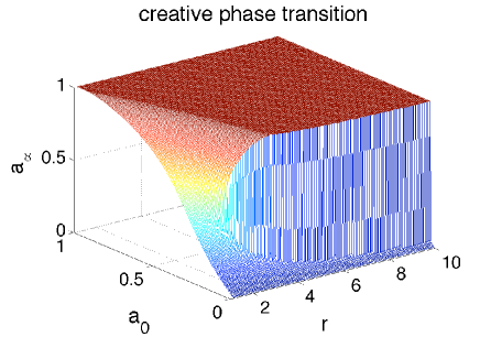
Figure 1: Phase diagram of the creative dynamics over the $r$-$a_{0}$ space.

III The destructive phase transition

In the dynamics studied so far diversity can only increase due to the positivity of the elements in $\alpha$. It is important to note that in this setting the phase transition can not be crossed in the backward direction. This is because of two reasons. First, the system forgets its initial condition $a_{0}$ once it has reached the (almost) fully populated state. This means that after everything has been produced one can not lower the initial set size any more. In terms of the Van der Waals gas equation analogy we can not lower the ’temperature’ and we can not cross the phase transition in the backward direction. Second, if $r$ is a homogeneous characteristic of the system then it is also impossible to manipulate the ’pressure’ of the system and we remain in the fully populated phase for ever.

The natural question thus arises what happens to the dynamics if one randomly kills a fraction of elements in the fully (or almost fully) populated phase. In the case that an element $k$ gets produced by a single pair $(i,j)$ and one of these – either $i$ or $j$ – gets killed, $k$ can not be produced any longer. We call the random removal of $i$ a primary defect, the result – here the stop of production of $k$ – is a secondary defect, denoted by $SD$. The question is whether there exist critical conditions of $r$ and a primary defect density $\delta_{0}$, such that cascading defects will occur.

As before we approach this question iteratively, by asking how many secondary defects will be caused by an initial set of $D_{0}$ randomly removed elements in the fully populated phase. We define the primary defect density $\delta_{0}\equiv D_{0}/d$. The possibility for a secondary defect happening to element $k$ requires that all productive pairs, which can produce $k$, have to be destroyed, i.e. at least one element of the productive pair has to be eliminated . This requires some ’book-keeping’ of the number of elements that partially have lost some of their productive pairs due to defects. We introduce a book-keeping set $G_{n}$ of sequences $g_{nl}$, $G_{n}=\{g_{n0},g_{n1},g_{n2},g_{n3},\cdots\}$, where $d\,g_{nl}$ denotes the number of elements that have lost $l$ ways to be produced (i.e. productive pairs), given that initially $n$ elements have been eliminated.

To be entirely clear, let us introduce the first defect. This defect will on average affect $2r$ productive pairs in the system, i.e., there will be $2r$ elements that loose one way of being produced . We naturally assume $d\gg d\delta_{0}\gg r>1$, and disregard the vanishingly small probability that one element looses two or more of its productive pairs by one primary defect.

Before the first defect we have $G_{0}=\{1,0,0,\cdots\}$, meaning that there are $d$ entities that have lost none of their producing pairs. The first defect will decrease this number $d\to d-2r$, i.e., we get $2r$ elements that have lost one of their producing pairs. Consequently we find $G_{1}=\{1-p,p,0,0,\cdots\}$, where $p$ is defined as $p\equiv 2r/d$. Now, defecting the second element will affect another $2r$ elements through their producing pairs. This time we affect an element that has lost none of its producing pairs with probability $1-p$, and with probability $p$ we affect an element that already has lost one of its producing pairs. Iterating this idea of subsequent defects leads to the recurrence relations

$$g_{n+1\,0}=g_{n\,0}\,(1-p)\qquad{\rm and}\qquad g_{n+1\,k}=g_{n\,k}+\left(g_{n\,k-1}-g_{n\,k}\right)\,p\quad.$$ (7)

It is easy to show that $g_{n\,k}$ follows a binomial law, $g_{n\,k}=\left(\begin{array}[]{c}n\\ k\end{array}\right)p^{k}(1-p)^{n-k}$. The number of secondary defects after $n$ introduced defects, denoted by $SD_{n}$, is just the number of all entities that have lost all of their (on average) $r$ producing pairs and can be estimated by $d\,\sum_{k\geq r}g_{n\,k}$. Defining

$$SD_{n}=\sum_{k\geq r}g_{n\,k}\quad,$$ (8)

one finds the update equation for $SD_{n}$ by inserting (7) into (8),

$$SD_{n+1}=SD_{n}+pg_{n\,r-1}\quad.$$ (9)

Now, if $d\,\delta_{0}$ and $d\,\delta_{1}$ are the numbers of primary and secondary defects respectively, one has to identify

$$\delta_{1}=SD_{d\delta_{0}}\quad.$$ (10)

This is nothing but

$$\begin{array}[]{lll}\delta_{1}&=&p\sum_{n\geq r}^{d\,\delta_{0}}g_{n\,r-1}=p\sum_{n\geq r}^{d\,\delta_{0}}\left(\begin{array}[]{c}n\\ r-1\end{array}\right)p^{r-1}(1-p)^{n-r+1}\quad.\end{array}$$ (11)

Since we assume $d\gg d\delta_{0}\gg r>1$, Stirling’s approximation is reasonable, $\ln(n!)\sim n\ln(n)-n+\frac{1}{2}\ln(2\pi n)$, so that the binomial coefficient is approximated by, $\left(\begin{array}[]{c}n\\ m\end{array}\right)\sim\left(\frac{n}{m}\right)^{m}e^{m}(2\pi m)^{-1/2}$, where $(1-m/n)^{n-m}\sim\exp(-m)$, for $n\gg m$. Further one can approximate $(1-p)^{n-r+1}\sim\exp(-np)$. Inserting these approximations into Eq. (11), and replacing the sum by an integral one gets

$$\delta_{1}=\frac{p^{r}}{\sqrt{2\pi}}(r-1)^{\frac{1}{2}-r}e^{r-1}\int_{r}^{d\,\delta_{0}}\,dx\,x^{r-1}e^{-xp}\quad.$$ (12)

Since $p\,d\delta_{0}=2\,r\,\delta_{0}$, and by approximating $p\,r\sim 0$ (for the lower limit) we rewrite the integral

$$\int_{r}^{d\,\delta_{0}}\,dx\,x^{r-1}e^{-xp}\sim p^{-r}\int_{0}^{2r\delta_{0}}\,dy\,y^{r-1}e^{-y}\quad,$$ (13)

and we can finally compute

$$\delta_{1}=\gamma(r)f(r,\delta_{0})\delta_{0}^{r}\quad,$$ (14)

with

$$\begin{array}[]{lll}\gamma(r)&=&\frac{1}{r}\frac{(2r)^{r}}{\sqrt{2\pi}}(r-1)^{\frac{1}{2}-r}e^{r-1}\\ &&\\ f(r,\delta_{0})&=&\sum_{n=0}^{\infty}\frac{1}{n!}\frac{r}{r+n}(-2r\delta_{0})^{n}\quad.\end{array}$$ (15)

Here $f$ is obtained by expanding the exponential in the integral of Eq. (13) into a Taylor series.

What remains to be done is to iterate Eq. (14). There are two possible ways of doing so. In the first iteration scheme we think of collecting the primary and secondary defects together and assume that we would start with a new primary defect set of size $\delta_{0}^{\prime}=\delta_{0}+\delta_{1}$. The tertiary defects therefore would be estimated by $\delta_{2}=\delta_{1}^{\prime}-\delta_{1}$, where $\delta_{1}^{\prime}$ are the secondary defects associated with $\delta_{0}^{\prime}$. This leads to the recursive scheme (A),

$$\Delta_{n}\equiv\sum_{k=1}^{n}\delta_{k}\quad,\qquad\delta_{n+1}=\gamma(r)f(r,\Delta_{n})\Delta_{n}^{r}-\Delta_{n}+\delta_{1}\quad({\rm A}).$$ (16)

The second way to iterate Eq. (14) is to assume that we use the $d\delta_{1}$ secondary defects as primary defects on the smaller (rescaled) system $d(1-\delta_{0})$ so that we look at a new primary defect-ratio $\delta_{0}^{\prime}=\delta_{1}/(1-\delta_{0})$. The result $\delta_{1}^{\prime}$ then has to be rescaled inversely to give the tertiary defects in the original scale, i.e. $\delta_{2}=(1-\delta_{0})\delta_{1}^{\prime}$. Iterating this idea leads to the recurrence relation (B),

$$\Delta_{n}\equiv\sum_{k=1}^{n}\delta_{k}\quad,\qquad\delta_{n+1}=\gamma(r)\left(1-\Delta_{n-1}\right)^{1-r}f\left(r,\frac{\delta_{n}}{1-\Delta_{n-1}}\right)\delta_{n}^{r}\quad({\rm B}),$$ (17)

with $\Delta_{0}\equiv 0$.

The result in terms of a phase diagram of the two possible iteration schemes (A) and (B) is given in Fig. 2 (a) and (b), respectively. The asymptotic defect size $\delta_{\infty}$ (for $t\to\infty$) is shown as a function of the parameters $r$ and the initial defect density $\delta_{0}$. As before a clear phase transition is visible, meaning that at a fixed value of $r$ there exists a critical number of initial defects at which the system will experience a catastrophic decline of diversity. Unfortunately, an analytical solution for the asymptotic iterations of Eq. (14) seems to be beyond the capabilities of the authors. It is interesting that complete destruction of diversity (plateau in Fig. 2) not very large values of $\delta_{0}$ are necessary.

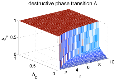
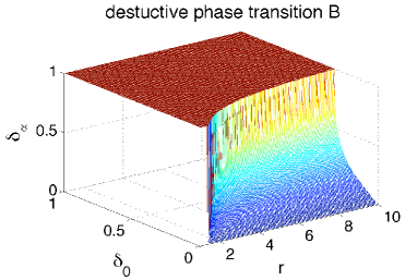
Figure 2: Phase diagram for the defect dynamics for two ways of iterating Eq. (14) described in the text.

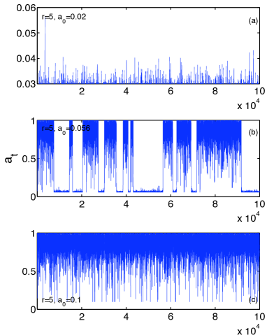
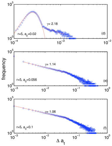
Figure 3: Time series and time increment distribution of the coupled dynamics for a fixed $r=5$ and fixed Poissonian rates $\eta$ and $\chi^{\pm}$. The variable varied is $a_{0}=0.02,0.056$, and $0.1$. Red lines are fits to power laws with slopes $\gamma$, and a Poissonian resembling the creative driving noise in (d). Note the change of scale here.

IV Combined dynamics: Creative gales of deconstruction

To become more realistic, since we have now established the existence of phase transitions in both the creative and destructive regimes, and are equipped with the update equations for the respective cases Eqs. (2) and (14), it is natural to couple these update equations and to study the combined dynamics. The relevant variable now becomes the diversity in the system as a function of time, $a_{t}$. However, the question how this should be done is neither trivial nor uniquely determined.

One realistic scenario might be that at any point in time some goods/species/elements may come into being spontaneously and others go extinct at certain rates. First, for the introduction of new elements we introduce a stochastic rate, $\chi^{+}>0$ of a Poisson process, so that $(d-a_{t})\chi^{+}_{t}$ new species may be expected in one time unit. Note, that there are $d-a_{t}$ ’un-populated’ elements in the system. These randomly created elements are elements that did not get produced through (re)combination or substitution of existing ones, but are ’out of the blue’ inventions. The natural time unit we are supplied with is one creative generation $a_{t}\to a_{t+1}$. The spontaneous creation may eventually increase the critical threshold and the system may transit into the highly diverse phase (think of this process to randomly alter $a_{0}$ in the creative update dynamics).

On the other hand there are spontaneous processes that destroy or remove species at a stochastic rate, $\chi^{-}>0$ (Poisson process), such that about $a_{t}\chi^{-}_{t}$ new defects may be expected per time unit. It can not be assumed a priori that the iterative accumulation of secondary defects in the system, as described above, operates at the same time scale as the spontaneous or the deterministic creative processes.

For making an explicit choice we may assume that during one time unit there happen $\eta_{t}$ generations of secondary defects, taking into account the relative ratio of innovative and secondary defect generations processed per time unit. We assume that $\eta_{t}$ can be modeled by a Poisson process whose rate, $\left<\eta_{t}\right>=\eta$ becomes a parameter of the model. For the computations below we have chosen $\eta=0.1$.

When we look at the way secondary defects evolve in generations we are left with a culminated number of secondary defects $\Delta_{\eta_{t}\,t}$ after $\eta_{t}$ generations and a remainder $\delta_{\eta_{t}\,t}$, which would have to be added to $\Delta_{\eta_{t}\,t}$ in the next defect-generation, $\eta_{t}+1$ but which – by assumption – is falling into the book-keeping of the next creative-generation time step $t+1$. What we say is that during time step $t\to t+1$, there are $\Delta^{-}a_{t}=d\Delta_{\eta_{t},t}$ species removed from the system, where $\Delta_{m\,t}=\sum_{k=0}^{m-1}\delta_{k\,t}$ is the cumulated ratio of secondary defect ratios $\delta_{k\,t}$ of defect-generation $k$ at time step $t$. The remaining defects of generation $\eta_{t}$ have to be accounted for in the next time step together with the newly introduced spontaneous defects, so that $\delta_{0\,t+1}=\frac{a_{t}}{d}\chi^{-}_{t}+\delta_{\eta_{t},t}$. The update of defect generations now can be performed $\eta_{t}$ times according to

$$\delta_{m+1\,t}=\left(1-\Delta_{m\,t}\right)\gamma_{r}f(r,\tilde{\delta}_{m\,t})\tilde{\delta}_{m\,t}^{r}\quad,$$ (18)

where we have considered the rescaling approach (B) to secondary defect generations. A similar equation can be derived for scheme (A). For convenience of notation we write for the rescaled defect ratios, $\tilde{\delta}_{m\,t}\equiv\frac{\delta_{m\,t}}{1-\Delta_{m\,t}}$. If now, by coincidence, the remaining defects from the last time step and the spontaneously introduced defects are sufficiently many and there are enough defect-generations $\eta_{t}$ processed in that time step, the culminating secondary defects may lead to a break down of the system from the high to the low diversity regime.

All that is left is to insert this dynamics into the creative update equation. To do so we first note that without defects, $\Delta a_{t}$ depends on both $a_{t}$ and $a_{t-1}$. However, due to the occurring defects $a_{t-1}$ will not remain what it was when $t$ becomes updated to $t+1$, but will be decreased by the occurring defects in this time span. For this reason it is convenient to introduce a new variable $b_{t}$ which takes the place of $a_{t-1}$ in the coupled update process. More precisely, $b_{t+1}\equiv a_{t}-\Delta^{-}a_{t}$. For the growth condition to be well defined we require $a_{t}>b_{t}$, which is guaranteed by $a_{t+1}=b_{t+1}+\Delta^{+}a_{t}$ where

$$\Delta^{+}a_{t}\equiv\frac{r}{d}\left(1-\frac{a_{t}}{d}\right)\left(a_{t}^{2}-b_{t}^{2}\right)+(d-a_{t})\chi^{+}_{t}\quad,$$ (19)

is the number of deterministically (by the creative update law) and spontaneously introduced species in the creative-generation $t$. This sort of coupling allows to take a look at how diversity of systems may evolve over time, driven by the spontaneous creation and destruction processes $\chi^{\pm}$, which may reflect exogenous influences, while on the other hand the average number of defect-generations $\eta$ per creative generation $t$, and the average number of productive pairs per species $r$ express endogenous properties of the system, i.e. whether the defects process slow or fast ($\eta$), and the average dependency ($r$) of the catalytic network.

We study the resulting timeseries for this dynamics for several values of $r$, $a_{0}$, $\eta$, and $\chi^{\pm}$. In Fig. 3, by fixing $r=5$ and the Poisson rates $\eta$, and $\chi^{\pm}$ and by varying $a_{0}$ from 0.01 to 0.1, we cross the creative phase transition line from the sub-critical to the fully populated phase. At $a_{0}=0.056$ we observe a flip-flop transition between the two phases. The flip-flop transitions happen over very short time intervals. In Fig. 3 (b) the increment distribution of $\Delta a_{t}\equiv a_{t}-a_{t-1}$ is shown. It is clearly seen that the distribution is power law whenever the super-critical phase is sufficiently populated. The Poissonian driving in the creative dynamics in the sub-critical region is clearly seen for $a_{0}=0.002$ in Fig. 3 (d). By power-law fits to the exponents in the deconstructive regime, we observe a sign for an existence of a Zipf law, i.e. $\gamma\sim 1$.

V Conclusion

We have shown the existence of a new phase transition in systems capable of evolutionary dynamics. Given that the system is in its highly diverse state, the introduction of relatively little primary removal of elements can cause drastic declines in diversity. We have further proposed a dynamical model to study timeseries of diversity in systems governed by the evolution equation (1) under the influence of external spontaneous creation and destruction processes. We emphasize that we strictly stick to the structure of Eq. (1) and do not discuss variants, such as the beautiful work of jain . In contrast they have studied a linear version (resembling catalytic equations), however with an explicit ’selection’ mechanism incorporated in a dynamic rule table.

As the main result of this present work we re-discover what J.A. Schumpeter has heuristically and qualitatively described as creative gales of deconstruction. More importantly we are able to quantify the dynamics of such systems. As an example destructive processes can be quantified in real world situations by bankruptcies of firms. In this context the existence of a power law and in particular empirical evidence for a Zipf law – similar to the one resulting from our model – has been found in zipf . As in the work of jain we observe the importance of different time scales in the coupled dynamics. In our approach we have incorporated this aspect by noting that creation and destruction do not work necessarily on the same time scales. Let us mention as a final comment that the results do of course not only apply to technological evolution but to any biological, social, or physical system governed by the evolution equation, Eq. (1).

References

- [1] S.A. Kauffman, The origins of order, (Oxford University Press, London, 1993).
- [2] M. Nowak, Evolutionary dynamics: exploring the equations of life, (Belknap Press, Mass., 2006).
- [3] M. Eigen, P. Schuster, The hypercycle, (Springer Verlag, Berlin, 1979).
- [4] W. Fontana, in Artificial life II, edited by C.G. Langton, C. Taylor, J.D. Farmer, S. Rasmussen (Addison Wesley, Redwood City, CA, 1992), pp. 159-210.
- [5] J.D. Farmer, S.A. Kauffman, N.H. Packard, Physica D 22, 50-67 (1986).
- [6] P.F. Stadler, W. Fontana, J.H. Miller, Physica D 63, 378 (1993).
- [7] S.J. Gould, The structure of evolutionary theory (Harvard University Press, Cambridge Mass., 2002).
- [8] R. Hanel, S.A. Kauffman, S. Thurner, Phys. Rev. E 77, 036117 (2005).
- [9] J.A. Schumpeter, Theorie der wirtschaftlichen Entwicklung, (Wien, 1911).
- [10] S. Jain and S. Krishna, Phys. Rev. Lett. 81, 5684-5687 (1998); Proc. Natl. Acad. Sci. USA 99, 2055-2060 (2002).
- [11] Y. Fujiwara, Physica A 337, 219-230 (2004).