Lower branch coherent states in shear flows: transition and control

Abstract

Lower branch coherent states in plane Couette flow have an asymptotic structure that consists of $O(1)$ streaks, $O(R^{-1})$ streamwise rolls and a weak sinusoidal wave that develops a critical layer, for large Reynolds number $R$. Higher harmonics become negligible. These unstable lower branch states appear to have a single unstable eigenvalue at all Reynolds numbers. These results suggest that the lower branch coherent states control transition to turbulence and that they may be promising targets for new turbulence prevention strategies.

Recent experiments indicate that the smallest amplitude necessary to trigger transition to turbulence in pipe flow scales with the inverse of the Reynolds number $R$, at least for a class of large scale perturbations HJM03 ; PhysToday04 . That $R^{-1}$ scaling, and other characteristics of the perturbations, are shown here to be consistent with a class of unstable 3D traveling wave solutions of the Navier-Stokes equation recently discovered in all canonical shear flows W98 ; W01 ; IT01 ; W03 ; FE03 ; WK04 . These new coherent solutions arise through saddle-node bifurcations at $R=R_{sn}$. At that onset Reynolds number, the solutions capture the form and length scales of the coherent structures that have long been observed in the near wall region of turbulent shear flows W03 . For $R>R_{sn}$, the solutions separate into upper and lower branches. For relatively low $R>R_{sn}$, a single traveling wave upper branch may capture the key statistics of turbulent shear flows remarkably well W03 ; JKSN05 ; science04 . Here it is shown that the lower branch solutions in plane Couette flow obey the $R^{-1}$ scaling and evidence is provided that these states form the ‘backbone’ of the phase space boundary separating the basin of attraction of the laminar flow from that of the turbulent flow, and are therefore directly connected with transition to turbulence W97 ; IT01 ; W03 .

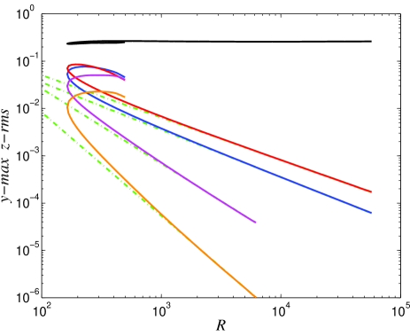
Figure 1: Amplitude of $x$-Fourier modes for a 3D steady state in plane Couette flow vs. $R$ for $(\alpha,\gamma)=(1,2)$. Top to bottom: $O(1)$ streak $u_{0}(y,z)\!-\!\bar{u}(y)$, $O(R^{-0.9})$ fundamental mode $|w_{1}|$, $O(R^{-1})$ streamwise rolls $(v_{0},w_{0})$ and $o(R^{-1})$ $|\mbox{\boldmath${v}$}_{2}|$ and $|\mbox{\boldmath${v}$}_{3}|$. Continued beyond $R=6168$ by dropping all harmonics. $R_{sn}\approx 164$ is the turning point where lower and upper branch solutions coalesce.

Incompressible fluid flow is governed by the Navier-Stokes equations

$$\partial_{t}\mbox{\boldmath${v}$}+\mbox{\boldmath${v}$}\cdot\mbox{\boldmath${\nabla}$}\mbox{\boldmath${v}$}+\mbox{\boldmath${\nabla}$}p=R^{-1}\nabla^{2}\mbox{\boldmath${v}$},\quad\mbox{\boldmath${\nabla}$}\cdot\mbox{\boldmath${v}$}=0,$$ (1)

where $\mbox{\boldmath${v}$}(\mbox{\boldmath${r}$},t)$ is the fluid velocity at point ${r}$ and time $t\geq 0$, $p(\mbox{\boldmath${r}$},t)$ is the mechanical pressure that enforces incompressibility and $R>0$ is the Reynolds number which is a non-dimensionalized inverse viscosity. The mean flow is in the ${\bf{e}}_{x}$ direction in a channel with parallel walls at $y=\pm 1$. Plane Couette flow (PCF) is driven by the motion of these walls so $\mbox{\boldmath${v}$}=\pm{\bf{e}}_{x}$ at $y=\pm 1$, for all $x,z,t$, in which case $\mbox{\boldmath${v}$}=y{\bf{e}}_{x}$ is the laminar solution of (1). That solution is linearly stable for all $R>0$ KLH94 . Periodic boundary conditions are imposed in the wall-parallel directions $x$ and $z$ with fundamental wavenumbers $\alpha$ and $\gamma$, respectively. Technical details can be found in W03 .

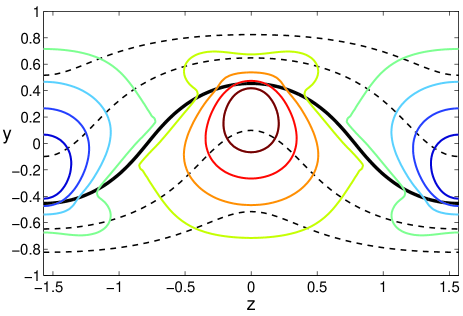
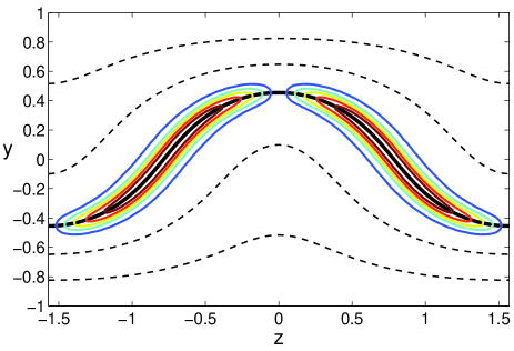
Figure 2: Contours of $v_{0}(y,z)$ (solid, top) and $|v_{1}(y,z)|$ (solid, bottom) both with contours of $u_{0}(y,z)=[-2:2]/3$ (dashed) for $(\alpha,\gamma,R)=(1,2,50171)$. The critical layer $u_{0}(y,z)=0$ is shown as a bold solid curve in both plots.

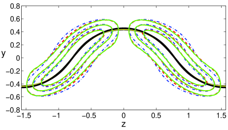
Figure 3: Contours of $|v_{1}|$ for $(\alpha,\gamma)=(1,2)$ at $R=50171$ (solid) and $12637$ (dashed) stretched by $R^{1/3}$ factors along curves normal to $u_{0}$-contours to match $|v_{1}|$ contours at $R=3079$ (dash-dot). The (almost overlapping) black and yellow solid curves show $u_{0}(y,z)=0$ at the 3 $R$’s.

For traveling wave solutions, the velocity field is Fourier decomposed in the $x$-direction as

$$\mbox{\boldmath${v}$}(\mbox{\boldmath${r}$},t)=\mbox{\boldmath${v}$}_{0}(y,z)+\left(\sum_{n=1}^{\infty}\!e^{in\theta}\mbox{\boldmath${v}$}_{n}(y,z)+c.c.\right)$$ (2)

where $\theta=\alpha(x-ct)$, $c$ is the constant wave velocity and $c.c.$ denotes complex conjugate. The $0$-mode $\mbox{\boldmath${v}$}_{0}(y,z)=(u_{0},v_{0},w_{0})$ consists of streamwise rolls $(0,v_{0},w_{0})$ with $\partial_{y}v_{0}+\partial_{z}w_{0}=0$ kinematically decoupled from the streamwise component $u_{0}$. The latter consists of an $x$ and $z$ averaged mean flow $\overline{u}(y)$ and streaks $u_{0}(y,z)-\overline{u}(y)$.

Symmetric lower branch traveling waves in plane Couette flow (for which $c=0$) have been continued to high $R$ by Newton’s method as in W98 ; W01 ; W03 . Figure 1 shows the scaling of the amplitudes of the various elements constituting such solutions as functions of $R$. The streaks $u_{0}(y,z)-\overline{u}(y)$ tend to a non-zero constant while the amplitude of the rolls $(0,v_{0}(y,z),w_{0}(y,z))$ scales like $1/R$ as $R\to\infty$. The fundamental mode $\mbox{\boldmath${v}$}_{1}(y,z)$ has an approximate $R^{-0.9}$ scaling, while the 2nd and 3rd harmonics scale approximately like $R^{-1.6}$ and $R^{-2.2}$ respectively. Higher harmonics decay faster and are not shown. This separation between the harmonics suggests that the 2nd and higher harmonics become insignificant for large $R$. Indeed, the solution was continued beyond $R=6168$ by dropping all harmonics with no significant change (none detectable on fig. 1). This is unusual: as $R$ is increased, the numerical resolution can be decreased in the $x$-direction. This is only true for the continuation of the lower branch solutions, and the catch is that the structure of the lower branch in the $(y,z)$-plane becomes more complex because the fundamental $\mbox{\boldmath${v}$}_{1}$ develops a critical layer, as discussed hereafter.

Figure 2 illustrates the structure of the lower branch steady state. The streaky flow $u_{0}(y,z)$ and the rolls $(0,v_{0},w_{0})$ remain large scale and their structure becomes independent of $R$; $v_{0}$ has a simple updraft at $z=0$ and downdraft at $z=\pm\pi/\gamma$ that sustain the $z$ modulation of $u_{0}(y,z)$ (recall that $u_{0}=\pm 1$ at $y=\pm 1$ in PCF). But the fundamental mode $\mbox{\boldmath${v}$}_{1}$ concentrates about the critical layer $u_{0}(y,z)=c$ ($c=0$ for these states in PCF). Critical layers are well-known in the context of the 2D, linear theory of shear flows M86 . Here the critical layer is a surface in 3D space and it is nonlinearly coupled to the $0$-mode $\mbox{\boldmath${v}$}_{0}(y,z)$. When the higher harmonics become negligible and $|v_{0}|,|w_{0}|\ll|u_{0}|$, the equation for the fundamental mode simplifies to W95a ; W97 ; B84

$$\left[i\alpha(u_{0}-c)\mbox{\boldmath${v}$}_{1}+(\mbox{\boldmath${v}$}_{1}\cdot\mbox{\boldmath${\nabla}$}u_{0}){\bf{e}}_{x}\right]e^{i\theta}=\\ -\mbox{\boldmath${\nabla}$}(p_{1}e^{i\theta})+R^{-1}\nabla^{2}\left(\mbox{\boldmath${v}$}_{1}e^{i\theta}\right),$$ (3)

with $\mbox{\boldmath${\nabla}$}\cdot\left(\mbox{\boldmath${v}$}_{1}e^{i\theta}\right)=0$. For high $R$, the solutions develop an $R^{-1/3}$ critical layer in the neighborhood of $u_{0}(y,z)-c=0$ that results from the balance between $\alpha(u_{0}-c)=\alpha(\mbox{\boldmath${r}$}-\mbox{\boldmath${r}$}_{c})\cdot\mbox{\boldmath${\nabla}$}u_{0}+O(|\mbox{\boldmath${r}$}-\mbox{\boldmath${r}$}_{c}|^{2})$ and $R^{-1}\nabla^{2}$, so if $\delta$ is the critical layer thickness, we must have $\alpha\delta|\mbox{\boldmath${\nabla}$}u_{0}|\sim R^{-1}\delta^{-2}$ and $\delta\sim(\alpha|\mbox{\boldmath${\nabla}$}u_{0}|R)^{-1/3}$ near $u_{0}(y,z)-c=0$. Figure 3 confirms that critical layer scaling for the lower branch steady state in PCF.

The nonlinear coupling W97 ; W03 between the fundamental $\mbox{\boldmath${v}$}_{1}$, with its critical layer structure, and the rolls $(v_{0},w_{0})$ provides a challenge for the development of a full asymptotic theory of the lower branch states that would be able to predict the amplitude scaling of the fundamental mode. If $\mbox{\boldmath${v}$}_{1}$ remained a large scale structure, its amplitude would have to scale like $R^{-1}$ in order for its nonlinear self-interaction to balance the viscous diffusion of the $R^{-1}$ streamwise rolls $v_{0}$ W95a ; W97 . The development of a critical layer scale complicates the analysis and different norms and components have different scalings. Nonetheless, an asymptotic theory appears feasible and the present numerical data is clear and its implications are significant: the lower branch states tend to a relatively simple but non-trivial quasi-2D singular asymptotic state as $R\to\infty$ that is not a solution of the Euler equation (eqn. (1) with $R^{-1}=0$), and that is not the laminar flow $\mbox{\boldmath${v}$}=y{\bf{e}}_{x}$ either. So the lower branch states do not bifurcate from the laminar flow, not even at $R=\infty$. The data presented is for $(\alpha,\gamma)=(1,2)$ however identical features hold for other $(\alpha,\gamma)$ values.

Turning now to a stability analysis of the lower branch coherent states we find that these states are distinguished not only by their asymptotic structure but also by their stability characteristics. Our eigenmode analysis of the 3D lower branch steady state in plane Couette flow, up to $R=12000$, show that they have a single, real unstable eigenvalue shown in figure 4 for $(\alpha,\gamma)=(1.14,2.5)$. This state is most unstable at $R\approx 342$ then the unstable eigenvalue steadily decreases approximately as $R^{-0.48}$ for larger $R$. Furthermore, the corresponding eigenfunction is in the same shift-reflect and shift-rotate symmetries (W03, , eqns. (24),(26)) as the lower branch state. This is not true for the upper branch states which develop new bifurcations and unstable modes as $R$ increases.

These stability results were obtained using both a direct calculation of the eigenvalues of the full Jacobian in the doubly symmetric subspace of the lower branch state with an ellipsoidal truncation of the Fourier-Chebyshev representation W03 , and an iterative calculation in the full space using the Arnoldi algorithm and the ChannelFlow code with cubic truncation channelflow . The leading unstable and least stable eigenvalues matched to 5 or 6 significant digits. We have also investigated subharmonic instabilities through numerical simulations in a double-sized box with fundamental wavenumbers $\alpha/2$ and $\gamma/2$. Sample simulations with ‘random’ perturbations did not reveal further instabilities, however a more systematic approach using the Arnoldi algorithm revealed a weakly unstable subharmonic in $x$. For $R=1000$ and $(\alpha,\gamma)=(1.14,2.5)$, the fundamental instability shown in fig. 4 has growth rate $0.03681$ while the subharmonic instability has growth rate $0.005248\pm i\,0.02245$. The analysis of this subharmonic mode is left for future study.

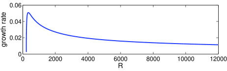
Figure 4: The single unstable eigenvalue of the lower branch state $(\alpha,\gamma)=(1.14,2.5)$ as function of $R$. Asympotic scaling is $\approx O(R^{-0.48})$. There is an extra complex conjugate pair near the onset $R_{sn}\approx 218$.

Thus, in the one-period domain with fundamental wavenumbers $(\alpha,\gamma)$, the lower branch state is an unstable equilibrium with a 1D unstable manifold. Therefore its stable manifold splits the phase space into two parts, at least locally. The evolution of disturbances in the one-period domain, starting on the 1D unstable manifold of the lower branch on either side of the stable manifold is illustrated in fig. 5. These numerical simulations were performed using ChannelFlow in the full phase space and show the time evolutions in the energy input-energy dissipation plane, both normalized by their laminar values. For plane Couette flow, the normalized energy input rate is equal to the normalized drag, that is, the drag at the walls normalized by their laminar value. Perturbations starting on one side of the stable manifold gently decay back to the linearly stable laminar flow $\mbox{\boldmath${v}$}=y{\bf{e}}_{x}$ while perturbations on the other side of the stable manifold shoot to a turbulent state. Figure 5 also shows the upper branch sister of the lower branch state which, as stated earlier, is located in phase space much closer to the ‘turbulent’ state. The decay of perturbed lower branch states back to the laminar flow follows a standard two-step evolution. First, the fundamental mode $\mbox{\boldmath${v}$}_{1}$, with its critical layer structure, disappears and the flow relaxes to an $x$-independent state that consists of streamwise rolls $(0,v_{0},w_{0})$ and streaks $u_{0}(y,z)$ and slowly decays back to the laminar flow on a long viscous time scale. Perturbations that shoot to a turbulent state follow a much more rapid ‘breakdown’ with high dissipation rate (about 13 on fig. 5) then settle to a turbulent state with energy input and dissipation rates of about $4.4$ (for $(\alpha,\gamma,R)=(1,2,1000)$).

These results suggest that the lower branch stable manifold is the boundary separating the basin of attraction of the laminar state from that of the turbulent state and therefore that they may be the key states controlling transition to turbulence. Our results have focused on symmetric steady states in plane Couette flow but there is evidence of a similar role for lower branch traveling waves in plane Poiseuille flow IT01 and pipe flow KT07 . Recent work by Viswanath V07-2 complements our work by showing that perturbations of the laminar flow in the form of streamwise rolls of the right threshold amplitude + small 3D noise do get attracted to a lower branch state before shooting to turbulence. We expect the symmetric lower branch state to play a key role for transition in plane Couette flow but there exist other asymmetric lower branch traveling wave states as well as periodic orbits V07-2 ; V07-1 ; KK01 , each of which may play a similar ‘transition-backbone’ role, locally in phase space. We conjecture that the permanent states (steady states, traveling waves and periodic orbits) most relevant to transition to turbulence will contain $R^{-1}$ streamwise rolls. It may be possible to trigger transition with smaller disturbances but we suspect that such disturbances would necessarily lead to the formation of $R^{-1}$ rolls and approach toward a lower branch state with $R^{-1}$ rolls prior to transition along the unstable manifold of the lower branch state.

 

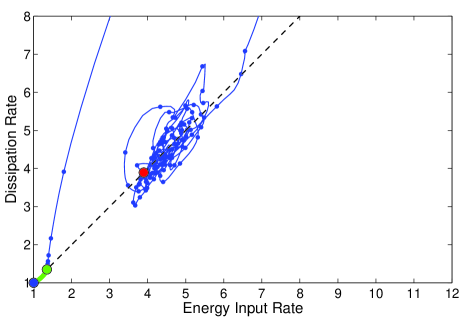
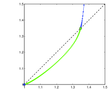
Figure 5: Energy input/dissipation rate starting near the lower branch fixed point $(\alpha,\gamma,R)=(1,2,1000)$ on its unstable manifold. In one direction, the flow goes to turbulence while in the other direction it relaminarizes. The dot spacing is $\triangle t=5$. The blue marker at (1,1) is the laminar flow, green marker at (1.35,1.35) is the lower branch state and the red marker at (3.89,3.89) is its upper branch sister.

The extreme low dimensionality of the lower branch unstable manifold suggests a new approach to turbulence control. Turbulence control strategies roughly fall into 2 categories: either prevent nonlinear breakdown of the linearly stable laminar flow, or push the fully nonlinear turbulent flow back to laminar. A new strategy might be to put the flow on the lower branch equilibria and keep it there by controlling its very few unstable modes. There is a small drag penalty to do so since lower branch states have a net drag that is 30 to 40% higher than the laminar state as $R\to\infty$ but that is a massive drag reduction compared to the turbulent state. This control strategy is related to, but quite distinct from the strategies proposed in KAWA05 and CossuPRL06 . Streaks are used in CossuPRL06 to efficiently deform the laminar base flow in order to prevent the linear instability of boundary layer flow. In KAWA05 strategies are considered to push the turbulent flow onto the laminar side of the stable manifold of a lower branch unstable periodic solution in order to relaminarize the flow. The current proposal is to put the flow on the unstable lower branch equilibrium and keep it there by controlling its single unstable eigenmode.

- [1] B. Hof, A. Juel, and T. Mullin. Scaling of the turbulence transition threshold in a pipe. Phys. Rev. Lett., 91:244502, 2003.
- [2] R. Fitzgerald. New experiments set the scale for the onset of turbulence in pipe flow. Physics Today, 57(2):21–23, 2004.
- [3] F. Waleffe. Three-dimensional coherent states in plane shear flows. Phys. Rev. Lett., 81:4140–4148, 1998.
- [4] F. Waleffe. Exact coherent structures in channel flow. J. Fluid Mech., 435:93–102, 2001.
- [5] T. Itano and S. Toh. The dynamics of bursting process in wall turbulence. J. Phys. Soc. Japan, 70:703–716, 2001.
- [6] F. Waleffe. Homotopy of exact coherent structures in plane shear flows. Phys. Fluids, 15:1517–1543, 2003.
- [7] H. Faisst and B. Eckhardt. Traveling waves in pipe flow. Phys. Rev. Lett., 91:224502, 2003.
- [8] H. Wedin and R.R. Kerswell. Exact coherent structures in pipe flow. J. Fluid Mech., 508:333–371, 2004.
- [9] J. Jimenez, G. Kawahara, M.P. Simens, and M. Nagata. Characterization of near-wall turbulence in terms of equilibrium and ‘bursting’ solutions. Phys. Fluids, 17:015105 (16pp.), 2005.
- [10] B. Hof, C.W.H. van Doorne, J. Westerweel, F.T.M. Nieuwstadt, H. Faisst, B. Eckhardt, H. Wedin, R.R. Kerswell, and F. Waleffe. Experimental observation of nonlinear traveling waves in turbulent pipe flow. Science, 305(5690):1594–1598, 2004.
- [11] F. Waleffe. On a self-sustaining process in shear flows. Phys. Fluids, 9:883–900, 1997.
- [12] G. Kreiss, A. Lundbladh, and D. S. Henningson. Bounds for threshold amplitudes in subcritical shear flows. Journal of Fluid Mechanics, 270:175–198, July 1994.
- [13] S.A. Maslowe. Critical layers in shear flows. Ann. Rev. Fluid Mech., 18:405–432, 1986.
- [14] F. Waleffe. Hydrodynamic stability and turbulence: Beyond transients to a self-sustaining process. Stud. Applied Math., 95:319–343, 1995.
- [15] D.J. Benney. The evolution of disturbances in shear flows at high Reynolds numbers. Stud. Appl. Math., 70:1–19, 1984.
- [16] J. F. Gibson. Channelflow: a spectral Navier-Stokes simulator in C++. Technical report, Georgia Institute of Technology, 2006. http://www.channelflow.org.
- [17] R.R. Kerswell and O.R. Tutty. Recurrence of traveling waves in transitional pipe flow. J. Fluid Mechanics (submitted), arxiv.org/physics/0611009, 2007.
- [18] D. Viswanath. The dynamics of transition to turbulence in plane Couette flow. arxiv.org/physics/0701337, 2007.
- [19] D. Viswanath. Recurrent motions within plane Couette turbulence. J. Fluid Mech., 2007 (to appear).
- [20] G. Kawahara and S. Kida. Periodic motion embedded in Plane Couette turbulence: regeneration cycle and burst. J. Fluid Mech., 449:291–300, 2001.
- [21] G. Kawahara. Laminarization of minimal plane Couette flow: Going beyond the basin of attraction of turbulence. Physics of Fluids, 17(4):041702, 2005.
- [22] J.H.M. Fransson, A. Talamelli, L. Brandt, and C. Cossu. Delaying transition to turbulence by a passive mechanism. Physical Review Letters, 96(6):064501, 2006.