The convolution theorem for nonlinear optics

Abstract

We have expressed the nonlinear optical absorption of a semiconductor in terms of its linear spectrum. We determined that the two-photon absorption coefficient in a strong DC-electric field of a direct gap semiconductor can be expressed as the product of a differential operator times the convolution integral of the linear absorption without a DC-electric field and an Airy function. We have applied this formalism to calculate the two-photon absorption coefficient and nonlinear refraction for GaAs and ZnSe using their linear absorption and have found excellent agreement with available experimental data.

A fundamental limitation in non-linear spectroscopy is the requirement for large peak laser intensities because a coherent $N$-photon process ($N\geq 2$) has a small cross section. With the limited availability of continuous laser sources having broad bandwidths and good coherence, nonlinear spectroscopy is challenging. In contrast linear absorption cross sections are much larger, especially in semiconductors close to a critical point (Van Hove singularities). Therefore, it would be ideal if the nonlinear properties, such as the two-photon absorption and nonlinear refraction of a semiconductor, could be predicted from their linear spectrum, which is relatively straightforward to obtain. In this Letter, we present a theoretical approach to predict the two-photon absorption spectrum of a direct gap semiconductor based only on its linear absorption spectrum close to the band-edge. The formalism developed here also gives information about the role of a DC-electric field on the nonlinear optical response of semiconductors. We have also applied the Kramers-Kronig relation to calculate the nonlinear refraction and have obtained excellent agreement with the available experimental data for $GaAs$ and $ZnSe$ direct-gap semiconductors. This theory could be of great significance towards identifying promising nonlinear optical materials for application in diverse areas such as optical switching and optical limiting.

The effect of electric field on the dielectric constant of solids has been extensively investigated in the past Tharmalingam (1963); Morgan (1966); Yacoby (1968); Aspnes (1967); Enderlein and Keiper (1967); French (1968). The effect, known as the Franz-Keldysh (FK) effect Franz (1958); Keldysh (1965), has been used as a tool in spectroscopy to modulate the energy gap and resolve details of the band structure otherwise embedded in a broadband background Aspnes and Rowe (1970); Aspnes (1980); Yu and Cardona (1996); Seraphin and Hess (1965). Recently, we reported the calculation of the nonlinear absorption coefficient in the presence of a very strong electric field for direct as well as indirect gap semiconductors and extended the formalism to the N-photon process Garcia (2006); Garcia and Kalyanaraman (2006). At the heart of the calculation is the use of a modified Volkov wavefunction that includes the effect of the electric field in one direction (Airy Function), and uses the S-matrix to calculate the N-photon transition rate in first-order perturbation theory. We worked in the effective mass approximation and assumed that the momentum matrix elements were independent of electron-hole wave vector k. We also assumed that the optical field only modified the final energy of the electron-hole pair. Finally, we considered an isotropic solid with a full valence band and an empty conduction band. The resulting generalized N-photon absorption coefficient in the presence of a DC-electric field was given by Garcia (2006):

$$\beta^{(N)}=\frac{\alpha_{b}f^{1/3}}{2^{2N-1}\pi}\left[\frac{8\pi e^{2}E_{\mu}}{n_{o}m_{c}^{2}c\omega^{4}}\right]^{N-1}\left[\frac{N(2N-3)!!}{((N-1)!)^{3}}\right]\left(\frac{m_{\mu}}{\hbar^{2}}\right)^{N}\int_{\epsilon_{o}^{(N)}}^{\infty}(\epsilon-\epsilon_{o}^{(N)})^{N-1}\mid Ai(\epsilon)^{2}\mid d\epsilon$$ (1)

where $E_{\mu}=\left(\hbar^{2}e^{2}F^{2}/2m_{\mu}\right)^{1/3}$ is the characteristic energy of the DC electric field $F$, $m_{\mu}$ is the electron effective mass, $m_{c}$ is mass of the electron in the conduction band, $n_{o}$ is the semiconductor index of refraction, $Ai(\epsilon)$ is the Airy function, and $f$, $\alpha_{b}$, and $\epsilon_{o}^{(N)}$ are given by: $f=\frac{2eFm_{\mu}}{\hbar^{2}}$; $\alpha_{b}=\frac{8\pi^{2}}{n_{o}c}\frac{\mid P_{vc}\mid^{2}e^{2}}{m_{o}^{2}\omega}$; and $\epsilon_{o}^{(N)}=\frac{E_{g}-N\hbar\omega}{E_{\mu}}$, where $m_{o}$ is the electron bare mass, and $P_{vc}$ is the interband momentum matrix elements. Using the following property of the Airy function Aspnes (1967):

$$\int_{o}^{\infty}t^{n}\mid Ai(t+x)\mid^{2}dt=\frac{n}{2n+1}\left[\frac{1}{2}\frac{d^{2}}{dx^{2}}-2x\right]\int_{o}^{\infty}t^{n-1}\mid Ai(t+x)\mid^{2}dt$$ (2)

the integral in Eq. 1 can be reduced after successive applications of Eq. 2 and using the below property:

$$\int_{0}^{\infty}\mid Ai(t+\epsilon_{o}^{(N)}\mid^{2}dt=\frac{2.4^{2/3}}{\pi}\int_{0}^{\infty}t^{\frac{1}{2}}Ai\left(t+\frac{E_{g}-N\hbar\omega}{\Omega}\right)dt$$ (3)

obtained from Abramowitz and Stegun (1972), where $\Omega=4^{-1/3}E_{\mu}$. As a consequence, the $N$-photon absorption coefficient $\beta^{(N)}$, Eq. 1, can be expressed in terms of the linear absorption as:

$$\beta^{(N)} = \frac{1}{2^{2N-1}\omega}\left[\frac{8\pi e^{2}E_{\mu}m_{\mu}}{\hbar^{2}n_{o}m_{c}^{2}c\omega^{4}}\right]^{N-1}\left[\frac{N(2N-3)!!}{\left[(N-1)!\right]^{2}\prod_{i=1}^{N}(2i-1)}\right]\left[\frac{1}{2}\frac{d^{2}}{d\epsilon_{o}^{(N)2}}-2\epsilon_{o}^{(N)}\right]^{N-1}\times$$ (4)

$$\int\beta^{(1)}(E^{{}^{\prime}})\frac{\omega^{{}^{\prime}}}{\Omega}Ai\left(\frac{E^{{}^{\prime}}-N\hbar\omega}{\Omega}\right)dE^{{}^{\prime}}$$

where $\beta^{(1)}$ is given by:

$$\beta^{(1)}=\frac{\alpha_{b}}{(2\pi)^{2}}\left[\frac{2m_{\mu}}{\hbar^{2}}\right]^{3/2}(E^{{}^{\prime}}-E_{g})^{1/2}=\frac{\alpha_{b}^{{}^{\prime}}(2m)^{3/2}}{(2\pi)^{2}\hbar^{2}}\frac{1}{E^{{}^{\prime}}}(E^{{}^{\prime}}-E_{g})^{1/2}$$ (5)

where we have redefined $\alpha_{b}$ such that the new $\alpha_{b}^{{}^{\prime}}$ and $E_{g}$ can be used as fitting parameters for the linear absorption. We see that Eq. 4 reduces to the well-know convolution theorem for $N=1$ Aspnes et al. (1968). We call Eq. 4 the $N$-photon absorption convolution theorem (i.e. the nonlinear convolution theorem) and view the differential operator as the $N$-photon absorption operator. In the case of $N=2$, the two-photon absorption coefficient is given by:

$$\beta^{(2)}=\frac{2}{3}\frac{\pi e^{2}E_{\mu}m_{\mu}}{\hbar^{2}n_{o}m_{c}^{2}c\omega^{5}}\left[\frac{1}{2}\frac{d^{2}}{d\epsilon_{o}^{(2)2}}-2\epsilon_{o}^{(2)}\right]\int_{-\infty}^{\infty}\beta^{(1)}(E^{{}^{\prime}})\frac{\omega^{{}^{\prime}}}{\Omega}Ai\left(\frac{E^{{}^{\prime}}-2\hbar\omega}{\Omega}\right)dE^{{}^{\prime}}$$ (6)

Eq. 6 contains a very remarkable result: the two-photon absorption is given by a convolution of the linear absorption. So if the spectrum of the linear absorption close to the band edge is known/measured then Eq. 6 can be used to generate the nonlinear absorption spectrum of the semiconductor. Also, using the familiar Kramers-Kronig (KK) relationship for nonlinear optics Sheik-Bahae et al. (1991) along with Eq. 6 we get:

$$n^{(2)}(\omega,F)=\frac{c}{\pi}\int_{0}^{\infty}\frac{\beta^{(2)}(\omega,F)}{\omega^{{}^{\prime}2}-\omega^{2}}d\omega^{{}^{\prime}}$$ (7)

for the nonlinear refraction.

Recently, there have been reports on the development of a new technique to measure the nonlinear absorption in a broad spectral range using Z-scan and a supercontinuum laser source Balu et al. (2005); He et al. (2002). Using this technique, the spectral distribution of the two-photon absorption for $ZnSe$ was measured. To test the above theory, we have calculated the two-photon absorption for $GaAs$ and $ZnSe$ semiconductors using Eq. 6. First, as shown in Fig. 1(a), the absorption coefficient for $GaAs$ was estimated using Eq. 5 and using $\alpha_{b}^{{}^{\prime}}$ and $E_{g}$ as fitting parameters, with low temperature experimental values taken from Palik (1985) (where the absorption edge is dominant). Table. 1 shows the values used in our calculation and the results for the energy gap and $\alpha_{b}^{{}^{\prime}}$. From the above result we calculated the two-photon absorption and the nonlinear refraction and compared it to the experimentally measured values Van Stryland et al. (1985); Hurlbut et al. (2007), as shown in Fig. 1(b) and Fig. 1(c). We have done a similar analysis for $ZnSe$ and the results for the linear absorption are shown in Fig. 2(a), with experimental data taken from Sop . The two-photon absorption and nonlinear refraction are shown in Fig. 2(b) and (c) respectively, with experimental values taken from Balu et al. (2005). In our calculations, we have used a characteristic energy of the DC field $E_{\mu}=1/10\times E_{g}$ in order to minimize band bending and allow comparison with the zero field case ($F=0$). The excellent agreement is indeed quite remarkable, especially when considering that the experimental absorption data for $ZnSe$ was taken from known values of $n$ and $k$ at room temperature Sop , and related to the absorption coefficient through $\alpha=(\frac{\omega}{n_{O}c})Im(\epsilon),$ where $\epsilon=n^{2}+k^{2}+2ink$, is the complex dielectric function.

In conclusion, we have explored some of the mathematical structures of the N-photon absorption process in the presence of a very strong DC-field. We have found that the nonlinear absorption can be expressed as the product of an N-photon operator times the linear absorption coefficient. This is, to our knowledge, the first time that nonlinear processes have been viewed as a consequence of a single photon process rescaled to an energy gap given by $E_{g}/N$. We also found that because of this relation, results such as the convolution theorem, and KK can be introduced naturally. Finally, we applied this formalism to two well known semiconductors ($GaAs$ and $ZnSe$) and found excellent agreement with experimental measured trends. This approach can be of great value in predicting nonlinear properties solely from measurements of linear properties.

RK acknowledges support by the National Science Foundation through grant # DMI-0449258.

Figure captions

1. Fig. 1. Comparison of experimental (symbols) and theoretical data (line) for GaAs. (a) linear absorption Palik (1985) and fit from our theory. (b) Nonlinear absorption. (c) Nonlinear refractive index. The experimental data for $\beta^{(2)}$ and $n_{2}$ was taken from Van Stryland et al. (1985); Hurlbut et al. (2007).

2. Fig. 2. Comparison of experimental (symbols) and theoretical data (line) for ZnSe. (a) linear absorption Sop and fit from our theory. (b) Nonlinear absorption. (c) Nonlinear refractive index. The experimental data for $\beta^{(2)}$ and $n_{2}$ was taken from Balu et al. (2005).

Table captions

1. Table of quantities used in the calculations. $m_{c}$, $m_{v}$, $m_{o}$ and $n_{o}$ are the known conduction electron mass, hole mass, electron mass and refractive index. $E_{g}$ and $\alpha_{b}^{{}^{\prime}}$ are energy gap and fitting parameter extracted from the linear absorption spectrum.

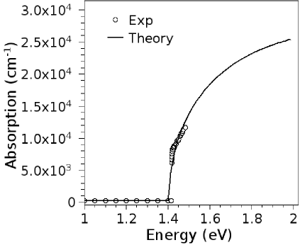
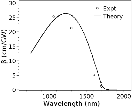
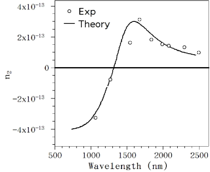
Figure 1: Comparison of experimental (symbols) and theoretical data (line) for GaAs. (a) linear absorption Palik (1985) and fit from our theory. (b) Nonlinear absorption. (c) Nonlinear refractive index. The experimental data for $\beta^{(2)}$ and $n_{2}$ was taken from Van Stryland et al. (1985); Hurlbut et al. (2007).

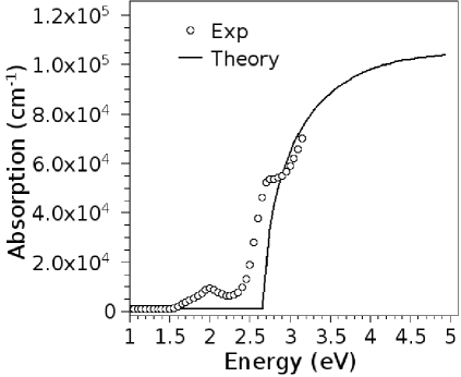
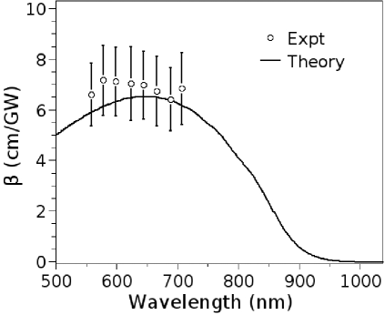
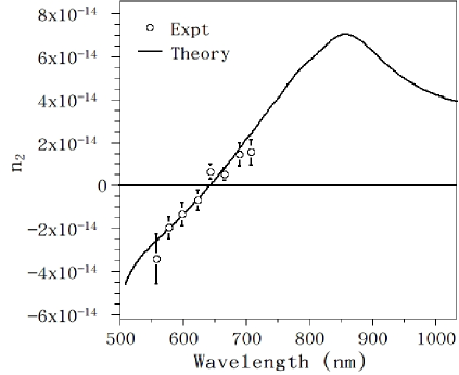
Figure 2: Comparison of experimental (symbols) and theoretical data (line) for ZnSe. (a) linear absorption Sop and fit from our theory. (b) Nonlinear absorption. (c) Nonlinear refractive index. The experimental data for $\beta^{(2)}$ and $n_{2}$ was taken from Balu et al. (2005).

	GaAs	ZnSe
$E_{g}$	1.403 eV	$2.67\,eV$
$m_{c}$	$0.067m_{o}$	$0.17m_{o}$
$m_{v}$	$0.68m_{o}$	$1.44m_{o}$
$n_{o}$	3.42	2.48
$\alpha_{b}^{{}^{\prime}}$	$2.43\times 10^{-6}(\frac{eV}{gm})^{1/2}erg$	$9.51\times 10^{-12}(\frac{eV}{gm})^{1/2}erg$

Table 1: Table of quantities used in the calculations. $m_{c}$, $m_{v}$, $m_{o}$ and $n_{o}$ are the known conduction electron mass, hole mass, electron mass and refractive index. $E_{g}$ and $\alpha_{b}^{{}^{\prime}}$ are energy gap and fitting parameter extracted from the linear absorption spectrum.

References

- Tharmalingam (1963) K. Tharmalingam, Phys. Rev. 130, 2204 (1963).
- Morgan (1966) T. N. Morgan, Phys. Rev. 148, 890 (1966).
- Yacoby (1968) Y. Yacoby, Phys. Rev. 169, 610 (1968).
- Aspnes (1967) D. E. Aspnes, Phys. Rev. 153, 972 (1967).
- Enderlein and Keiper (1967) R. Enderlein and R. Keiper, Phys. Stat. Sol. 19, 673 (1967).
- French (1968) B. T. French, Phys. Rev. 174, 991 (1968).
- Franz (1958) W. Franz, 13a, 484 (1958).
- Keldysh (1965) L. Keldysh, JETP 20, 1307 (1965).
- Aspnes and Rowe (1970) D. E. Aspnes and J. E. Rowe, Solid State Commun. 8, 1145 (1970).
- Aspnes (1980) D. E. Aspnes, Handbook of semiconductors (North-Holland, Amsterdam, 1980), vol. 2, p. 109.
- Yu and Cardona (1996) P. Y. Yu and M. Cardona, Fundamentals of semiconductors (Springer, New York, 1996), chap. 6, p. 305.
- Seraphin and Hess (1965) B. O. Seraphin and R. B. Hess, Phys. Rev. Lett. 14, 138 (1965).
- Garcia (2006) H. Garcia, Phys. Rev. B 74, 035212 (2006).
- Garcia and Kalyanaraman (2006) H. Garcia and R. Kalyanaraman, J. Phys. B: At. Mol. Opt. Phys. 39, 2737 (2006).
- Abramowitz and Stegun (1972) M. Abramowitz and I. A. Stegun, eds., Handbook of Mathematical Functions (National Bureau of Standards, Washington, D.C., 1972).
- Aspnes et al. (1968) D. E. Aspnes, P. Handler, and D. F. Blossey, Phys. Rev. 166, 921 (1968).
- Sheik-Bahae et al. (1991) M. Sheik-Bahae, D. Hutchings, D. Hagan, and E. Van Stryland, IEEE J. Quant. Elec. 27, 1296 (1991).
- Balu et al. (2005) M. Balu, J. Hales, D. Hagan, and E. Van Stryland, OPN 16, 28 (2005).
- He et al. (2002) G. He, T.-C. Lin, P. Prasad, R. Kannan, R. Vaia, and L.-S. Tan, Optics Exp. 10, 566 (2002).
- Palik (1985) E. Palik, Handbook of Optical Constants of Solids (Academic Press, NY, 1985).
- Van Stryland et al. (1985) E. W. Van Stryland, M. A. Woodall, H. Vanherzeele, and M. J. Soileau, Optics Lett. 10, 490 (1985).
- Hurlbut et al. (2007) W. C. Hurlbut, Y.-S. Lee, and K. L. Vodopyanov, Optics Lett. 32, 668 (2007).
- (23) SOPRA database, http://www.sopra-sa.com/.