Spectral and network methods in the analysis of correlation matrices of stock returns

Abstract

Correlation matrices inferred from stock return time series contain information on the behaviour of the market, especially on clusters of highly correlating stocks. Here we study a subset of New York Stock Exchange (NYSE) traded stocks and compare three different methods of analysis: i) spectral analysis, i.e. investigation of the eigenvalue-eigenvector pairs of the correlation matrix, ii) asset trees, obtained by constructing the maximal spanning tree of the correlation matrix, and iii) asset graphs, which are networks in which the strongest correlations are depicted as edges. We illustrate and discuss the localisation of the most significant modes of fluctuation, i.e. eigenvectors corresponding to the largest eigenvalues, on the asset trees and graphs.

, , , and

1 Introduction

The exact nature of interactions between stock market participants is not known but their manifestations in the performance of stocks are visible. Therefore it is natural to study correlation matrices of stock returns to learn about the internal structure of the market. This can be done by studying the spectral properties of correlation matrices or by constructing and studying weighted complex networks based on these matrices (see e.g. [1, 2, 3, 4] and references therein). Here, we compare these two approaches.

The paper is organised as follows: in Section 2 we give a short introduction to financial correlation matrices and their spectral properties. A comparison of the spectral properties and results obtained using asset trees and graphs is presented in Section 3. Summary and conclusions are given in Section 4.

2 Correlation matrix and its spectral properties

Our dataset consists of the split-adjusted daily closing prices of $N=116$ stocks, traded at the New York Stock Exchange (NYSE) for the time period from 13-Jan-1997 to 29-Dec-2000. This amounts to 1000 price quotes per stock. The equal time correlation matrix of logarithmic returns is constructed by

$$C_{ij}=\frac{\langle G_{i}G_{j}\rangle-\langle G_{i}\rangle\langle G_{j}\rangle}{\sigma_{i}\sigma_{j}},$$ (1)

where $\sigma_{i}=\sqrt{\langle G_{i}^{2}\rangle-\langle G_{i}\rangle^{2}}$, $G_{i}(t)=\ln P_{i}(t)-\ln P_{i}(t-1)$, $P_{i}(t)$ is the price of stock $i$ at time $t$ and the angular brackets denote time average. From Eq. 1 we see that the correlation matrix $C$ is the covariance matrix of the time series rescaled to have unit variance. These time series can be seen as $T$ realisations of a random vector $Z$ in $\mathbb{R}^{N}$, assuming that the elements of the time series are real numbers and we have $N$ time series of length $T$. By diagonalising $C$ we can find an orthogonal system of coordinates where the components of $Z$ do not correlate. These components are usually called the principal components. The elements of the diagonal matrix, the eigenvalues, implicate the variances of the corresponding principal components. In the following we denote the eigenvectors of $C$ by $x_{1},\ldots,x_{N}$ and the corresponding eigenvalues by $\lambda_{1},\ldots,\lambda_{N}$, where $\lambda_{1}>\ldots>\lambda_{N}$.

The eigenvectors can be thought to represent modes of fluctuation. The time series studied here are such that the rescaling makes them comparable with each other and this is clearly inherited to the principal components. Thus the eigenvalues reflect the significance of the corresponding modes of fluctuation.

The correlation matrix $C$ of $N$ assets has $N(N-1)/2$ distinct entries. Assuming that one determines an empirical correlation matrix from $N$ time series of length $T$ and $T$ is not very large compared to $N$, the entries of the correlation matrix are very noisy and the matrix is to a large extent random. Laloux et al. [5] and Plerou et al. [6] have studied the spectral properties of financial correlation matrices and concluded that only few eigenpairs carry real information. Their work suggests that the eigenvalues can be classified as follows:

1. The very smallest eigenvalues do not belong to the random part of the spectrum. The corresponding eigenvectors are highly localized, i.e., only a few assets contribute to them.

2. The next smallest eigenvalues (about 95 % of all eigenvalues) form the “bulk” of the spectrum. They or at least most of them correspond to noise and are well described by random matrix theory.

3. The largest eigenvalue is well separated from the bulk and corresponds to the whole market as the corresponding eigenvector has roughly equal components.

4. The next largest eigenvectors carry information about the real correlations and can be used in identifying clusters of strongly interacting assets.

3 Asset trees, asset graphs and eigenvector localisation

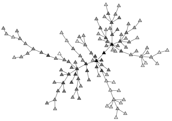
Figure 1: The asset tree, displaying the values of the components of the most significant mode of fluctuation, the market eigenvector $x_{1}$. The color of a node denotes the contribution of the corresponding component of $x_{1}$ to the length of the eigenvector. The largest component is colored black. For other nodes, linear scale is used such that white color indicates zero contribution.

In addition to spectral analysis, correlation matrices of stock return time series have recently been analyzed with network-related methods. The aim has been to uncover structure in the correlation matrix in the form of clusters of highly correlating stocks. In this section we discuss how the eigenvectors corresponding to the largest eigenvalues are localized with respect to clusters of stocks inferred using the asset tree [1, 2] and asset graph [7] approaches.

The maximal spanning tree of the stocks, later referred to as the asset tree, is a simply connected graph consisting of all $N$ stocks and $N-1$ edges such that the sum of the correlation coefficients between the endpoints of each edge is maximized. Fig. 1 displays the asset tree for our data set, together with the market eigenvector $x_{1}$, i.e., the most significant mode of fluctuation. The color of a node denotes the contribution of the corresponding eigenvector component to the length of the eigenvector (i.e., the square of the component). The linear color map is chosen such that white color indicates zero contribution and the largest component is denoted by black, shades of grey depicting smaller component values. We see that the most central nodes of the asset graph contribute most to the market eigenvector. This is rather natural, as the central nodes in the asset graph are known to be very large multisector companies or investment banks, which obviously fluctuate as their diversified investments [2].

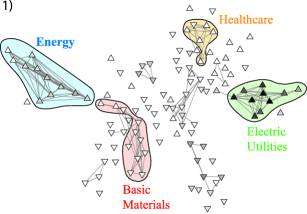
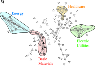
Figure 2: The asset graph for occupation $p=0.025$ and the localisation of $x_{2}$, $x_{3}$, $x_{4}$ and $x_{5}$ (panels 1-4, respectively). The orientation of the triangle at a node denotes the sign of the corresponding eigenvector component, and the color is determined as in Fig. 1. Clusters corresponding to these eigenvectors, identified by the clique percolation method, are denoted by the shaded background.

As discussed earlier by Mantegna [1] and Onnela et al. [2], the asset tree contains a lot information about the clustering of stocks. Therefore it is very interesting to compare the localization of the next most significant modes and the topology of the asset tree. From Fig. 2, where the nodes are plotted with the same coordinates as in Fig. 1 and the localisation of $x_{2}$, $x_{3}$, $x_{4}$ and $x_{5}$ is illustrated (panels 1-4, respectively), we see that these modes are mainly localised to branches of the asset tree. In these eigenvectors, unlike in the market eigenvector $x_{1}$, components of both signs exist. The sign of a component is denoted by the orientation (up or down) of the triangle at the corresponding node. According to the Forbes classification [8] the above mentioned branches approximately correspond to the Electric Utilities industry of the Utilities sector, the Energy sector, the Basic Materials sector and the Healthcare sector.

Onnela et al. [7] were the first to study the clustering of stocks using asset graphs constructed from correlation matrices of returns. An asset graph is constructed by ranking the non-diagonal elements of the correlation matrix $C$ in decreasing order and then adding a set fraction of links between stocks starting from the strongest correlation coefficient. The emergent network can be characterised by a parameter $p$, the ratio of the number of added links to the number of all possible links, $N(N-1)/2$. Evidently, the higher the value of $p$, the denser the resulting network; in our view the question of whether some specific value of $p$ yields the most informative structure is still open (see Ref. [7] for results obtained by sweeping the $p$ value). For the following analysis we have simply chosen $p=0.025$ as with this value the strongest clusters are clearly visible. In order to identify the visually apparent cluster structure, we have utilized the clique percolation method introduced by Palla et al. [9], using cliques of size three. The four clusters detected with this method, best corresponding to eigenvectors $x_{2},\ldots,x_{5}$ are illustrated in Fig. 2. The clusters are seen to mostly correspond to the above-mentioned industry sectors.

cluster vector $e_{c}$	$x_{1}$	$x_{2}$	$x_{3}$	$x_{4}$	$x_{5}$
Electric Utilities	0.2277	0.7117	-0.3585	0.0708	-0.4117
Energy	0.3026	0.3148	0.7190	-0.4299	0.0298
Basic Materials	0.3451	-0.0739	0.2859	0.6096	0.0762
Healthcare	0.2510	0.0388	-0.2691	-0.2416	0.5042

Table 1: The Euclidean inner products of the vectors describing the clusters and the eigenvectors $x_{1},\ldots,x_{5}$. The largest value of each row is bolded.

From Fig. 2 we see that $x_{2}$ and $x_{3}$ are rather strongly localised to the respective clusters; however, $x_{4}$ and especially $x_{5}$ no longer match the clusters well. The localisation of the market eigenvector $x_{1}$ and the following four eigenvectors is quantified in Table I, which displays the inner products of these eigenvectors and vectors depicting the clique percolation clusters. We have defined a normalized vector to depict each cluster such that $e_{c}=[e_{c}^{1},\ldots,e_{c}^{N}]^{T}$, where $e_{c}^{i}$ is constant for all components belonging to cluster $c$ and zero for other components. It is seen that $x_{1}$ is rather evenly distributed in the clusters, whereas $x_{2}$ and $x_{3}$ are mostly localised on the Electric Utilities and Energy clusters, respectively. Similarly $x_{4}$ and $x_{5}$ are mostly localised on the Basic Materials and Healthcare clusters. However, the difference to other clusters appears to become smaller with increasing eigenvector index. This is corroborated by analysis of further eigenvectors (not shown); with some exceptions the eigenvectors with higher indices appear less well localized with respect to clusters of the asset graph or branches in the asset tree.

4 Summary and conclusions

We have studied and compared how strongly correlated clusters of stocks are revealed as branches in the asset tree, as clusters in asset graphs, and as non-random eigenpairs of the correlation matrix. The eigenvector corresponding to the largest eigenvalue has roughly equal components, but the components corresponding to the most central nodes of the asset tree are on average somewhat larger than others. The eigenvectors corresponding to the next largest eigenvalues are to some extent localised on branches of the asset tree. When comparing the localization of these eigenvectors to clique percolation clusters, it is seen that the first few eigenvectors match the clusters rather well. However, their borders are “fuzzy” and do not define clear cluster boundaries. With increasing eigenvector index, the eigenvectors appear to localize increasingly less regularly with respect to the asset graph (or asset tree) topology. Hence it appears that identifying the strongly interacting clusters of stocks solely based on spectral properties of the correlation matrix is rather difficult; the asset graph method seems to provide more coherent results.

Acknowledgments

The authors would like to thank János Kertész and Gergely Tibély for useful discussions. This work has been supported by the Academy of Finland (the Finnish Center of Excellence program 2006-2011).

References

- [1] R. N. Mantegna, Eur. Phys. J. B 11, 193 (1999).
- [2] J.-P. Onnela, A. Chakraborti, K. Kaski, J. Kertész, and A. Kanto, Phys. Rev. E 68, 056110 (2003).
- [3] M. Tumminello, T. Aste, T. Di Matteo, and R.N. Mantegna, Proc. Natl. Acad. Sci. USA 102, 10421 (2005).
- [4] M. Tumminello, T. Aste, T. Di Matteo, and R. N. Mantegna, Eur. Phys. J. B. (2006), arxiv: physics/0605251.
- [5] L. Laloux, P. Cizeau, J.-P. Bouchaud, and M. Potters, Phys. Rev. Lett. 83, 1467 (1999).
- [6] V. Plerou, P. Gopikrishnan, B. Rosenow, L. A. N. Amaral, and H. E. Stanley, Phys. Rev. Lett. 83, 1471 (1999).
- [7] J.-P. Onnela, K. Kaski, and J. Kertész, Eur. Phys. J. B 38, 353 (2004).
- [8] Forbes at http://www.forbes.com, referenced in March-April 2002.
- [9] G. Palla, I. Derényi, I. Farkas, and T. Vicsek, Nature 435, 814 (2005).