Continuous macroscopic limit of a discrete stochastic model
for interaction of living cells

Abstract

In the development of multiscale biological models it is crucial to establish a connection between discrete microscopic or mesoscopic stochastic models and macroscopic continuous descriptions based on cellular density. In this paper a continuous limit of a two-dimensional Cellular Potts Model (CPM) with excluded volume is derived, describing cells moving in a medium and reacting to each other through both direct contact and long range chemotaxis. The continuous macroscopic model is obtained as a Fokker-Planck equation describing evolution of the cell probability density function. All coefficients of the general macroscopic model are derived from parameters of the CPM and a very good agreement is demonstrated between CPM Monte Carlo simulations and numerical solution of the macroscopic model. It is also shown that in the absence of contact cell-cell interactions, the obtained model reduces to the classical macroscopic Keller-Segel model. General multiscale approach is demonstrated by simulating spongy bone formation from loosely packed mesenchyme via the intramembranous route suggesting that self-organizing physical mechanisms can account for this developmental process.

Dec. 25, 2006

A large literature exists studying continuous limits of point-wise discrete microscopic models for biological systems. For example, the classic Keller-Segel PDE model of chemotaxis [1] was derived from a discrete model with point-wise cells undergoing random walk [2-5]. However, many biological phenomena require taking into account the finite size of biological cells, and much less work has been done on deriving macroscopic limits of microscopic models which treat cells as extended objects. The mesoscopic Cellular Potts Model (CPM), first introduced by Glazier and Graner [6, 7], has been used as a component of multiscale, experimentally motivated hybrid approaches, combining discrete and macroscopic continuous representations, to simulate, among others, morphological phenomena in the cellular slime mold Dictyostelium discoideum Pa , vascular development Merks and the proximo-distal increase in the number of skeletal elements in the developing avian limb Fram1 .

One of the earliest attempts at combining mesoscopic and macroscopic levels of description of cellular dynamics was described in turner2004 where the diffusion coefficient for a collection of noninteracting randomly moving cells was derived from a one-dimensional CPM. Recently a microscopic limit of subcellular elements model NewmanMathBioEng2005 was derived in the form of an advection-diffusion partial differential equation for cellular density. In previous papers alber1 ; alber2 we studied the continuous limit of 1D and 2D models of individual cell motion in a medium, in the presence of an external field but without contact cell-cell interactions.

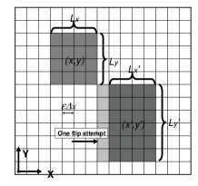
Figure 1: Cell representation in the two dimensional CPM. In this picture grey and white colors are used to indicate the cell body and ECM respectively. Cell can grow or shrink in $x$ and $y$ direction by adding or removing one row (or column) of pixels.

This paper describes a theoretical analysis leading to a continuous macroscopic limit of the two-dimensional mesocopic CPM with contact cell-cell interactions. Our approach, which is based on combining mesoscopic and macroscopic models, can be applied to studying biological phenomena in which a nonconfluent population of cells interact directly and via soluble factors, forming an open network structure. Examples include vasculogenesis Merks ; rupp ; szabo ; gamba and formation of trabecular, or spongy, bone cormack ; courtin ; tabor to be described below.

The CPM, defined on a multidimensional lattice, allows simulation of both cell-cell contact and chemotactic long distance interactions, along with extended cell representations. In deriving below our continuous model we assume that cells interact with one another subject to an excluded volume constraint. In the CPM a multidimensional integer index is associated with each lattice site (pixel) to indicate that a pixel belongs to a cell of particular type or medium. Each cell is represented by a cluster of pixels with the same index. Pixels evolve according to the classical Metropolis algorithm based on Boltzmann statistics, and the effective energy

$$E=E_{Adhesion}+E_{Perimeter}+E_{Field}.$$ (1)

Namely, if a proposed change in a lattice configuration results in energy change $\Delta E$, it is accepted with probability

$$\Phi(\Delta E)=\left\{\begin{array}[]{cc}1,&\Delta E\leq 0\\ e^{-}\frac{\Delta E}{T},&\Delta E>0,\end{array}\right.$$ (2)

where $T$ represents an effective boundary fluctuation amplitude of model cells in units of energy. Since the cells’ environment is highly viscous, cells move to minimize their total energy consistent with imposed constraints and boundary conditions. If a change of a randomly chosen pixels’ index causes cell-cell overlap it is abandoned. Otherwise, the acceptance probability is calculated using the corresponding energy change. If the change attempt is accepted, this results in changing location of the center of mass and dimensions of the cell.

In this paper we assume that each cell has a rectangular shape, that it moves or changes its shape by adding or removing a row or column of pixels (see Figure 1) and that cells come into direct contact with each other. They also interact with each other over long distances through producing diffusing chemicals and reacting to local chemical gradients (process called chemotaxis). Although we model adhesion between cells and the extracellular matrix (ECM), we neglect cell-cell adhesion and take into account cell-cell interaction from excluded volume constraint meaning that cells cannot occupy the same volume. Under these assumptions terms in the Hamiltonian (1) have the following forms. $E_{Adhesion}$ phenomenologically describes the net adhesion or repulsion between the cell surface and ECM and it is a product of the binding energy per unit length, $J_{CM}$, and the length of an interface between the cell boundary and ECM: $E_{Adhesion}=2J_{cm}(L_{x}+L_{y})$. $E_{\mathit{Perimeter}}$ defines an energy penalty function for dimensions of a cell deviating from the target values $L_{T_{x}}$ and $L_{T_{y}}$: $E_{Perimeter}=\lambda_{x}(L_{x}-L_{T_{x}})^{2}+\lambda_{y}(L_{y}-L_{T_{y}})^{2}$ where $\lambda_{x}$ and $\lambda_{y}$ are constants. Cells can move up or down gradients of both diffusible chemical signals (i.e., chemotaxis) and insoluble ECM molecules (i.e., haptotaxis) described by $E_{Field}=\mu\,c({\bf r})L_{x}L_{y},\;\;{\bf r}=(x,y)$ where $c(\bf r)$ is a local concentration of particular species of signaling molecules in the extracellular space and $\mu$ is an effective chemical potential.

Let $P({\bf r},{\bf L},t)$ denote the probability density for a rectangular cell with its center of mass at ${\bf r}$ to have dimensions ${\bf L}\equiv(L_{x},L_{y})$ at time $t.$ We use vectors ${\bf e}_{1,2}$ to indicate changes in $x$ and $y$ dimensions: ${\bf e}_{1}={\triangle r}(1,0),\ {\bf e}_{2}=\triangle r(0,1)$. Let us normalize the total probability to the number of cells: $\int P({\bf r},{\bf L},t)d{\bf r}d{\bf L}=N.$

Now assume that cells cannot occupy the same space. This implies that position ${\bf r}^{\prime}$ and size ${\bf L}^{\prime}$ of any neighboring cell should satisfy the following excluded volume conditions: $|x-x^{\prime}|\geq\frac{L_{x}+L_{x}^{\prime}}{2},$ $|y-y^{\prime}|\geq\frac{L_{y}+L_{y}^{\prime}}{2}.$

A discrete stochastic model of the cell dynamics under these conditions is described by the following master equation

$$P({\bf r},{\bf L},t+\epsilon^{2}\triangle t)=\sum_{j=1}^{2}\Big{\{}\big{[}\frac{1}{2}-\Phi_{j,l}({\bf r}-\frac{\epsilon}{2}{\bf e}_{j},{\bf L}+\epsilon{\bf e}_{j};{\bf r},{\bf L},t)$$

$$-\Phi_{j,r}({\bf r}+\frac{\epsilon}{2}{\bf e}_{j},{\bf L}+\epsilon{\bf e}_{j};{\bf r},{\bf L},t)-T_{l}({\bf r}+\frac{\epsilon}{2}{\bf e}_{j},{\bf L}-\epsilon{\bf e}_{j};{\bf r},{\bf L},t)$$

$$-T_{r}({\bf r}-\frac{\epsilon}{2}{\bf e}_{j},{\bf L}-\epsilon{\bf e}_{j};{\bf r},{\bf L},t)\big{]}P({\bf r},{\bf L},t)$$

$$+\Phi_{j,l}({\bf r},{\bf L};{\bf r}+\frac{\epsilon}{2}{\bf e}_{j},{\bf L}-\epsilon{\bf e}_{j},t)P({\bf r}+\frac{\epsilon}{2}{\bf e}_{j},{\bf L}-\epsilon{\bf e}_{j},t)$$

$$+\Phi_{j,r}({\bf r},{\bf L};{\bf r}-\frac{\epsilon}{2}{\bf e}_{j},{\bf L}-\epsilon{\bf e}_{j},t)P({\bf r}-\frac{\epsilon}{2}{\bf e}_{j},{\bf L}-\epsilon{\bf e}_{j},t)$$

$$+T_{l}({\bf r},{\bf L};{\bf r}-\frac{\epsilon}{2}{\bf e}_{j},{\bf L}+\epsilon{\bf e}_{j},t)P({\bf r}-\frac{\epsilon}{2}{\bf e}_{j},{\bf L}+\epsilon{\bf e}_{j},t)$$

$$+T_{r}({\bf r},{\bf L};{\bf r}+\frac{\epsilon}{2}{\bf e}_{j},{\bf L}+\epsilon{\bf e}_{j},t)P({\bf r}+\frac{\epsilon}{2}{\bf e}_{j},{\bf L}+\epsilon{\bf e}_{j},t)\Big{\}},$$ (3)

where $T_{l}({\bf r},{\bf L};{\bf r}^{\prime},{\bf L}^{\prime},t)$ and $T_{r}({\bf r},{\bf L};{\bf r}^{\prime},{\bf L}^{\prime},t)$ denote probabilities of transitions from a cell of length $L^{\prime}$ and center of mass at $r^{\prime}$ to a cell of dimensions $L$ and center of mass at $r$ without taking into account excluded volume principle. (Terms with $T_{l}$ and $T_{r}$ in Eq. (Continuous macroscopic limit of a discrete stochastic model for interaction of living cells) correspond to the case of decreasing cell size $|{\bf L}|<|{\bf L}^{\prime}|$ which justifies the neglect of excluded volume.) $\Phi_{j,l}({\bf r},{\bf L};{\bf r}^{\prime},{\bf L}^{\prime},t)$ and $\Phi_{j,r}({\bf r},{\bf L};{\bf r}^{\prime},{\bf L}^{\prime},t)$ are probabilities of transitions taking into account excluded volume. Subscripts $l$ and $r$ correspond to transitions by addition/removal of a row/colomn of pixels from the rear/lower and front/upper ends of a cell respectively. According to the CPM we have that $T_{l}(x,{\bf L};{\bf r}^{\prime},{\bf L}^{\prime})=T_{r}({\bf r},{\bf L};{\bf r}^{\prime},{\bf L}^{\prime})=\frac{1}{8}\Phi\Big{(}E({\bf r},{\bf L})-E({\bf r}^{\prime},{\bf L}^{\prime})\Big{)}$ where the factor of $1/8$ is due to the fact that there are potentially 8 possibilities for increasing or decreasing of $L_{x}$ and $L_{y}$.

We define $\Phi_{j,l}({\bf r},{\bf L};{\bf r}^{\prime},{\bf L}^{\prime})\equiv T_{l(r)}({\bf r},{\bf L};{\bf r}^{\prime},{\bf L}^{\prime})[1-\phi_{j,r(l)}({\bf r},\,{\bf L},t)]$ where $\phi_{j,r(l)}({\bf r},\,{\bf L},t)$ is the probability of another cell being in the immediate neighborhood of a given cell and, therefore, preventing an increase of that cells’ length or width (excluded volume). We neglect triple and higher order “collisions” between cells resulting in the following approximation formulas

$$\phi_{1,k}({\bf r},\,{\bf L},t)=(N-1)(\epsilon\triangle r)^{4}$$

$$\times\sum\limits_{{\bf L}^{\prime},y^{\prime}}\Theta\big{(}\frac{L_{y}+L^{\prime}_{y}}{2}-|y^{\prime}-y|\big{)}P({\bf r}^{\prime},{\bf L}^{\prime},t)\Big{|}_{x^{\prime}=x+s\frac{L_{x}+L^{\prime}_{x}}{2}}$$

$$\phi_{2,k}({\bf r},{\bf L},t)=(N-1)(\epsilon\triangle r)^{4}$$

$$\times\sum\limits_{{\bf L}^{\prime},x^{\prime}}\Theta\big{(}\frac{L_{x}+L^{\prime}_{x}}{2}-|x^{\prime}-x|\big{)}P({\bf r}^{\prime},{\bf L}^{\prime},t)\Big{|}_{y^{\prime}=y+s\frac{L_{y}+L^{\prime}_{y}}{2}}$$ (4)

where $s=1$ for $k=l$, $s=-1$ for $k=r$ and factor $N-1$ is due to pairwise cell collisions.

We found by using Monte Carlo simulations (not shown) that solutions of the master equation (Eq.$(\ref{pmasterxL1})$) with general initial conditions quickly converge to $P({\bf r},{\bf L},t)=P_{Boltz}({\bf r},{\bf L})p({\bf r},t)$ where $P_{Boltz}({\bf r},{\bf L})=Z({\bf r})^{-1}\exp(-\beta\triangle E_{length})$ is the Boltzmann distribution and $\triangle E_{length}=E({\bf r},{\bf L})-E_{min}=\lambda_{x}\tilde{L}_{x}^{2}+\lambda_{y}\tilde{L}_{y}^{2}+\tilde{L}_{x}\tilde{L}_{y}\mu c({\bf r})$ and $\tilde{\bf L}={\bf L}-{\bf L}^{(min)}$. Also, $E_{min}=E({\bf r},{\bf L}^{(min)})$ is the minimal value of the Hamiltonian (1) achieved at ${\bf L}={\bf L}^{(min)}$ and $Z({\bf r})=(2\epsilon\triangle r)^{2}\sum\limits_{{\bf L}}\exp(-\beta\triangle E_{length})\simeq\frac{{2\pi}}{\beta\sqrt{4\lambda_{x}\lambda_{y}-\mu^{2}c({\bf r})^{2}}},\ \epsilon\to 0$ is an asymptotic formula for a partition function.

The typical fluctuation of cell dimensions ($\tilde{L}_{x},\ \tilde{L}_{x}$) are determined by $\beta\lambda_{x(y)}\tilde{L}_{x(y)}^{2}\sim 1$. We now assume in addition that $\beta x_{0}^{2}\lambda_{x}\gg 1$ and $\quad\beta y_{0}^{2}\lambda_{y}\gg 1,$ where $x_{0}$ and $y_{0}$ are typical scales of $P$ with respect to $x$ and $y$. This means that $x_{0}\gg\tilde{L}_{x},\ y_{0}\gg\tilde{L}_{y}.$ We also assume that the concentration of chemoattractant $c({\bf r})$ is a slowly varying function of ${\bf r}$ on a scale of the typical cell’s length meaning that $x_{c}/L_{x}\gg 1,\quad y_{c}/L_{y}\gg 1,$ where $x_{c}$ and $y_{c}$ are typical scales for variation of $c({\bf r})$ in $x$ and $y$. We also make the additional biologically relevant assumption that $4\lambda_{x}\lambda_{y}\gg\mu^{2}c({\bf r})^{2}$ which means that change of typical cell size due to chemotaxis $(\delta L^{(chemo)}_{x},\delta L^{(chemo)}_{y})$ is small $|\delta L^{(chemo)}_{x(y)}|\ll L^{(min)}_{x(y)}.$ Under all above mentioned assumptions, the master Eq. $(\ref{pmasterxL1})$ is transformed in the limit $\epsilon\ll 1$ into an integro-differential equation describing evolution of the probability density $p({\bf r},t)$ for the location of the cellular center of mass

$$\partial_{t}p=D_{2}\partial^{2}_{\bf r}p-\chi_{0}\partial_{\bf r}\cdot\big{[}p\,\partial_{\bf r}c({\bf r})\big{]}$$

$$+\frac{D_{2}}{2}(N-1)\Big{\{}\partial_{x}[\psi_{x}p]+\partial_{y}[\psi_{y}p]\Big{\}}$$

$$\psi_{x}=\int\limits^{y+L_{y}^{(min)}}_{y-L_{y}^{(min)}}\big{[}p(x+L_{x}^{(min)},y^{\prime})-p(x-L_{x}^{(min)},y^{\prime})\big{]}dy^{\prime}$$

$$\psi_{y}=\int\limits^{x+L_{x}^{(min)}}_{x-L_{x}^{(min)}}\big{[}p(x^{\prime},y+L_{y}^{(min)})-p(x^{\prime},y-L_{y}^{(min)})\big{]}dx^{\prime}$$

$$\chi_{0}=-D_{2}\mu\beta L_{x}^{(min)}L_{y}^{(min)},$$ (5)

where $D_{2}=\frac{(\triangle r)^{2}}{16\triangle t},\partial^{2}_{\bf r}=\partial_{x}^{2}+\partial_{y}^{2},$ $\chi_{0}=-D_{2}\mu\beta L_{x}^{(min)}L_{y}^{(min)},\,\,\,L_{x}^{(min)}=L_{T_{x}}-\frac{J_{cm}}{\lambda_{x}},\,\,\,L_{y}^{(min)}=L_{T_{y}}-\frac{J_{cm}}{\lambda_{y}}$ and $\int p({\bf r})d{\bf r}=N$. Lastly, we couple this equation to an equation describing evolution of the external (chemotactic) field $c$

$$\partial_{t}c=D_{c}\partial^{2}_{\bf r}c-\gamma c+a\,p$$ (6)

where $D_{c},\gamma$ and $a$ are diffusion, decay and production rates of the field respectively. Note that the chemical is produced by cells.

If excluded volume is not taken into account (i.e. assuming $\psi_{x}=\psi_{y}=0$) Eqs. $(\ref{pottscontinuous2dex})$ and $(\ref{ceq2D})$ reduce to the classical Keller-Segel system KS which has a finite time singularity and which was used for modeling collapse (aggregation) of bacterial colonies BrennerConstantinKadanoff1999 . Addition of excluded volume significantly slows down collapse and, therefore, Eqs. $(\ref{pottscontinuous2dex})$ and $(\ref{ceq2D})$ can be used for simulating cellular aggregation for a much longer period of time. Spongy bone formation considered in this paper, is accompanied by secretion of a viscous or solid ECM (see below) which quickly stabilizes a transient or metastable arrangement of cells into a persistent microanatomy and therefore also prevents collapse.

Figure 2 demonstrates a very good agreement between typical CPM simulation and numerical solution of the continuous model $(\ref{pottscontinuous2dex})$ and $(\ref{ceq2D})$. Both simulations were performed on a rectangular domain $0\leq x,y\leq 100$ with simulation time $t_{end}=100$. Parameters were chosen as follows: $\triangle r=1$, $L_{T_{x}}=L_{T_{y}}=3$, $\lambda_{x}=\lambda_{y}=1.5$, $J_{cm}=2$, $\beta=15$, $\mu=0.1$, $D_{c}=3.0$, $\gamma=0.00025$ and $a=0.2$. The time interval between successive Monte Carlo steps was $\delta t=\epsilon^{2}\triangle t=0.0001,\;\epsilon=0.01$. Discrete form of the equation (6) was used to calculate the chemical field dynamics on a $200\times 200$ lattice with the time step $\Delta t_{c}=0.0125$ and initial chemical field chosen in the form of $c_{0}(x,y)=\frac{(x-70)^{2}+(y-60)^{2}}{400}$. The typical size of the mesh used in the continuous model was $1000\times 1000$ and the time step was $0.002$. A large number of CPM simulations have been run to guarantee a representative statistical ensemble. We assumed that at each time step each cell released chemical content $a\Delta t_{c}$ which was then distributed to four nearest chemical lattice sites.

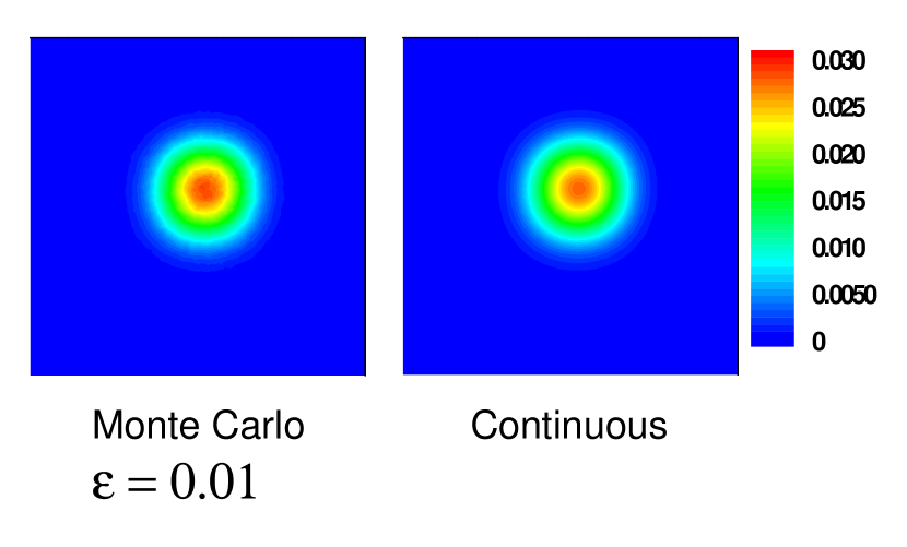
(a)

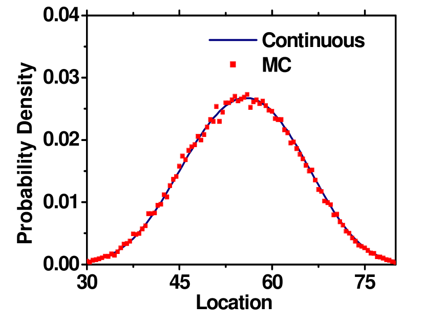
(b)

Figure 2: Comparison between mesoscopic CPM and macroscopic continuous model. (a) Plot of a two-dimensional probability density distributions for a CPM simulation of $12$ cells with $\epsilon=0.01$ and numerical solution $p(x,y,t)$ of the continuous Eq.$(\ref{pottscontinuous2dex})$. (b) Cross sections of $p_{cpm}(x_{0},y,t)$ and $p_{con}(x_{0},y,t)$ at $x_{0}=53.0$ as functions of $y$.

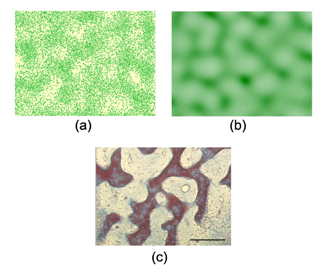
Figure 3: Simulation of spongy bone formation process. $\triangle r=1$, $L_{T_{x}}=L_{T_{y}}=0.6$, $\lambda_{x}=\lambda_{y}=1.5$, $J_{cm}=0.002$, $\beta=15$, $\mu=-0.1$, $D_{c}=0.5$, $\gamma=0.014$, $\Delta t_{c}=\epsilon^{2}\Delta t=0.01,\epsilon=0.1$, $t_{end}=180$. (a) Monte Carlo CPM simulation. $a=0.7$. $N=15000$ cells were randomly distributed in a domain $0\leq x,y\leq 100$ with initial chemical field at zero. (b) Numerical solution of the continuous model resulting from a uniform initial cell density distribution and with $5\%$ random fluctuation, $a=0.2$. (c) Histological section of developing spongy bone in the rat skull. Trichrome stain. Photographed from a section in the New York Medical College Histology slide collection. The effective magnification of this image is about 2x that of a and b. Scale bar: 100 micrometers.

In what follows, we illustrate the efficacy of the model by applying it to the formation of spongy bone via the intramembranous route. In this developmental phenomenon, which generates portions of the skull, maxilla and mandible in vertebrate organisms, bone cells, or osteoblasts, differentiate directly from loosely packed mesenchymal cells. The differentiating cells secrete TGF-beta which acts chemotactically, influencing cell migration while simultaneously inducing production of ECM Kanaan , which in developing bone is termed osteoid cormack .

Depending on local conditions, including initial cell density, the bone will progress to a dense state or stop at a spongy state, in which bony rods or trabeculae form a swiss-cheese-like network (see Figure 3c) that eventually contains marrow tissue originating from the circulation. Our mesoscopic and macroscopic model simulations which start with initially dilute populations of cells in a chemotactic field, subject to an excluded volume constraint, result in a transiently appearing set of interconnected multicellular trabeculae (see Figures 3a and 3b) similar to the experimental picture (Figure 3c). In particular, in the simulations and the developing tissue there are many nodes from which three branches extend, but few with larger numbers.

In summary, we have derived a macroscopic continuous model (Continuous macroscopic limit of a discrete stochastic model for interaction of living cells) from a mesoscopic two-dimensional CPM with excluded volume constraint and coupled it to a model of chemotaxis (6). Numerical simulations confirm a very good agreement between the CPM and macroscopic equations. Numerical analysis of the macroscopic model facilitated determination of conditions promoting formation of a lattice-like aggregation pattern. This permitted us to locate the parameter ranges within which the model cells in the CPM simulations behaved qualitatively like the living cells that form multicellular branches in spongy bone by intramembranous ossification(Figure 3c). In contrast to earlier suggestions that the trabecular arrangement of spongy bone is based on pre-existing vascular patterns Caplan , or later-forming patterns of mineral deposition courtin ; tabor , our results suggest that it can arise from the self-organizing behavior of mesenchymal cells interacting with their ECM.

This work was partially supported by NIH Grant No. 1R0-GM076692-01: Interagency Opportunities in Multiscale Modeling in Biomedical, Biological and Behavioral Systems NSF 04.6071 and NSF grants IBN-0344647, FIBR-0526854 and MRI DBI-0420980.

References

• (1) E.F. Keller and L.A. Segel, J. Theor. Biol. 30, 225 (1971).
• (2) W.Alt, J.Math Biol. 9, 147 (1980).
• (3) H.G. Othmer and A. Stevens, SIAM J. Appl. Math. 57 No.4 1044 (1997).
• (4) A. Stevens, SIAM J. Appl. Math. 61, 172 (2000).
• (5) T.J. Newman and R. Grima, Phys. Rev. E, 70, 051916 (2004).
• (6) F. Graner and J.A. Glazier, Phys. Rev. Lett. 69, 2013 (1992).
• (7) J.A. Glazier and F. Graner, Phys. Rev. E 47, 2128 (1993).
• (8) A.F.M. Marée and P. Hogeweg, Proc. Natl. Acad. Sci. U.S.A. 98, (7) 3879 (2001).
• (9) R.M.H. Merks et al., Dev. Biol. 289, 44 (2006).
• (10) R. Chaturvedi et al., J. R. Soc. Interface 2 237 (2005)
• (11) S. Turner, J.A. Sherratt, K.J. Painter, N.J. Savill, Phys. Rev. E 69, 021910 (2004).
• (12) T.J. Newman, Biosciences and Engeneering 2, 611 (2005).
• (13) M. Alber, N. Chen, T. Glimm, and P.M. Lushnikov, Phys. Rev. E. 73, 051901 (2006).
• (14) M. Alber, et al. Single Cell Based Models in Biology and Medicine, Birkhauser-Verlag (scheduled for publication in April 2007).
• (15) P.A. Rupp, A. Czirok, and C.D. Little, Development 131, 2887 (2004).
• (16) A. Szabo, E.D. Perryn and A. Czirok, Phys. Rev. Lett. 98, 038102 (2007).
• (17) A. Gamba et al., Phys. Rev. Lett. 90, 118101 (2003).
• (18) D. H. Cormack and A.W. Ham, Ham’s Histology, Lippincott (1987).
• (19) B. Courtin, A. M. Perault-Staub, and J. F. Staub, Acta Biotheor. 43, 373 (1995).
• (20) Z. Tabor, E. Rokita and T. Cichocki, Phys. Rev. E 66, 051906 (2002).
• (21) M.P. Brenner et al., Nonlinearity 12, 1071 (1999).
• (22) R.A. Kanaan and L.A. Kanaan, Med. Sci. Monit. 12, RA164 (2006)
• (23) A.I. Caplan and D.G. Pechak, Bone and mineral research, edited by W. A. Peck (Elsevier Science Publishers, New York, NY, 117 (1987)