Spherical Couette flow in a dipolar magnetic field

Abstract

We consider numerically the flow of an electrically conducting fluid in a differentially rotating spherical shell, in a dipolar magnetic field. For infinitesimal differential rotation the flow consists of a super-rotating region, concentrated on the particular field line $\mathcal{C}$ just touching the outer sphere, in agreement with previous results. Finite differential rotation suppresses this super-rotation, and pushes it inward, toward the equator of the inner sphere. For sufficiently strong differential rotation the outer boundary layer becomes unstable, yielding time-dependent solutions. Adding an overall rotation suppresses these instabilities again. The results are in qualitative agreement with the DTS liquid sodium experiment.

1 Introduction

Spherical Couette flow is the flow induced in a spherical shell by differentially rotating the inner and/or outer spheres. Despite its simplicity, this configuration yields a broad range of different flow patterns, which form an important part of classical fluid dynamics. Now suppose that the fluid is electrically conducting, and a magnetic field is imposed. Magnetohydrodynamic effects then arise, which can radically alter the flow structures from the previous nonmagnetic ones. In this paper we present numerical solutions of spherical Couette flow in a dipolar magnetic field, and compare them, at least qualitatively, with the DTS (Derviche Tourneur Sodium) liquid sodium experiment [1,2].

The mechanism whereby a magnetic field alters the flow is via the magnetic tension force, coupling fluid along the magnetic field lines. For a dipolar field, this singles out the particular field line $\mathcal{C}$ just touching the outer sphere at the equator [3]. Fluid inside $\mathcal{C}$ is coupled only to the inner sphere, and hence co-rotates with it, whereas fluid outside $\mathcal{C}$ is coupled to both spheres, and rotates at some intermediate rate. The shear layer on $\mathcal{C}$ separating the two regions scales as $Ha^{-1/2}$, where the Hartmann number $Ha$ is a measure of the strength of the imposed field.

However, this applies only if both boundaries are insulating. If the inner boundary is conducting, one obtains not a shear layer on $\mathcal{C}$, but rather a super-rotating jet, that is, a region of fluid rotating faster than either boundary [4,5]. The thickness of this jet still scales as $Ha^{-1/2}$, and the amount of super-rotation saturates at around 30% of the imposed differential rotation. Finally, if both boundaries are conducting, the amount of super-rotation does not saturate, but instead increases as $Ha^{1/2}$ [6,7].

So, one interesting aspect of the DTS experiment might be to study this super-rotation, and how it depends on the various parameters in the problem. However, no clear evidence for super-rotation was found, at least not on this particular field line $\mathcal{C}$. This in turn motivates us to reconsider this problem numerically, and attempt to reconcile the experimental results with the previous theoretical ones. We will find that the crucial feature is the inertial term $Re\,\bf U\cdot\nabla U$, which was not included in the previous theoretical studies, but which is certainly important in the experiment. Indeed, studying this regime where inertial effects can be as or even more important than magnetic effects was one of the main motivations in setting up the experiment. We show here that including inertia radically alters the flow patterns, and eliminates the special role previously played by the field line $\mathcal{C}$. For sufficiently large Reynolds numbers we obtain instabilities similar to ones found in the experiment. Finally, we show how an overall rotation suppresses these instabilities again, also in qualitative agreement with the experimental results.

2 Equations

In a reference frame co-rotating with the outer sphere, the suitably nondimensionalized equations are

$$\frac{\partial{\bf U}}{\partial t}+Re\,{\bf U\cdot\nabla U}+2E^{-1}\,{\bf\hat{e}}_{z}\times{\bf U}$$

$$=-\nabla p+\nabla^{2}{\bf U}+Ha^{2}\,Rm^{-1}\,(\nabla\times{\bf B})\times{\bf B},$$

$$Re^{-1}\,\frac{\partial{\bf B}}{\partial t}=Rm^{-1}\,\nabla^{2}{\bf B}+\nabla\times({\bf U\times B}),$$

together with $\nabla\cdot{\bf U}=0$ and $\nabla\cdot{\bf B}=0$. Length has been scaled by the outer sphere’s radius $r_{o}$, time by the viscous diffusive timescale $r_{o}^{2}/\nu$, and the flow $\bf U$ by $r_{i}\Delta\Omega$, where $r_{i}$ is the inner sphere’s radius, and $\Delta\Omega=\Omega_{i}-\Omega_{o}$ is the differential rotation between the inner and outer spheres. Note incidentally how the flow scale is not given by lengthscale/timescale. The scalings adopted here were chosen because they include the $\Delta\Omega\to 0$ limit of infinitesimal differential rotation in a particularly convenient form, simply as $Re\to 0$ in (7).

The Hartmann number

$$Ha=\frac{B_{0}r_{o}}{\sqrt{\mu\rho\nu\eta}},$$

where $\mu$ is the permeability, $\rho$ the density, $\nu$ the kinematic viscosity, and $\eta$ the magnetic diffusivity, is a measure of the strength $B_{0}$ of the imposed dipole field, at $r=1$, $\theta=\pi/2$ (where $r,\theta,\phi$ are standard spherical coordinates). $B_{0}$ is then also the scaling for the field $\bf B$.

The inverse Ekman number

$$E^{-1}=\frac{\Omega_{o}\,r_{o}^{2}}{\nu}$$

measures the outer sphere’s rotation rate, and the two Reynolds numbers

$$Re=\frac{\Delta\Omega\,r_{i}r_{o}}{\nu},\qquad Rm=\frac{\Delta\Omega\,r_{i}r_{o}}{\eta}$$

both measure the differential rotation rate, compared with the viscous and magnetic diffusive timescales, respectively.

The ratio $Rm/Re=\nu/\eta$ is a material property of the fluid, referred to as the magnetic Prandtl number $Pm$. For liquid sodium $Pm\sim 10^{-5}$. This extremely small value of $Pm$ means that $Re$ can be quite large while $Rm$ is still small. This allows us to further simplify the governing equations in the following way: Expand the field as

$${\bf B}={\bf B}_{0}+Rm\,{\bf b},$$

where ${\bf B}_{0}=2\cos\theta\,r^{-3}\,{\bf\hat{e}}_{r}+\sin\theta\,r^{-3}\,{\bf\hat{e}}_{\theta}$ is the imposed dipole field (now normalized to $|{\bf B}_{0}|=1$ at $r=1$, $\theta=\pi/2$), and $Rm\,{\bf b}$ is the induced field. Inserting (6) into (1-2) and neglecting $O(Rm)$ terms then yields

$$\frac{\partial{\bf U}}{\partial t}+Re\,{\bf U\cdot\nabla U}+2E^{-1}\,{\bf\hat{e}}_{z}\times{\bf U}$$

$$=-\nabla p+\nabla^{2}{\bf U}+Ha^{2}\,(\nabla\times{\bf b})\times{\bf B}_{0},$$

$$\nabla^{2}{\bf b}=-\nabla\times({\bf U\times B}_{0}),$$

which (by construction) no longer involves $Rm$ at all. That is, $Rm$ enters only in the meaning we ascribe to $\bf b$, but not in the equations we actually solve. The advantage of this small $Rm$ approximation is that the induction equation (8) is no longer time-stepped at all, but simply inverted at each time-step of the momentum equation (7). Filtering out the magnetic diffusive timescale in this way then allows for larger time-steps than would otherwise be possible.

The boundary conditions associated with (7) are

$${\bf U}=r\sin\theta\,{\bf\hat{e}}_{\phi}\quad{\rm at}\quad r=r_{i},\qquad{\bf U}=0\quad{\rm at}\quad r=r_{o}.$$

Those associated with (8) are a little more complicated. We begin by decomposing $\bf b$ as

$${\bf b}=\nabla\times(g\,{\bf\hat{e}}_{r})+\nabla\times\nabla\times(h\,{\bf\hat{e}}_{r}),$$

and expanding $g$ and $h$ in Legendre polynomials

$$g=\sum_{l}g_{l}(r,t)\,P_{l}(\cos\theta),\qquad h=\sum_{l}h_{l}(r,t)\,P_{l}(\cos\theta).$$

The boundary conditions at $r_{i}$ are then

$$\frac{d}{dr}\,g_{l}-\frac{l+1}{r}\,g_{l}=0,\qquad\frac{d}{dr}\,h_{l}-\frac{l+1}{r}\,h_{l}=0,$$

corresponding to a conducting inner sphere [8]. The boundary conditions at $r_{o}$ are

$$\epsilon\frac{d}{dr}\,\Bigl{(}rg_{l}\Bigr{)}+g_{l}=0,\qquad\frac{d}{dr}\,h_{l}+\frac{l}{r}\,h_{l}=0,$$

corresponding to a thin outer layer of relative conductance $\epsilon$. That is, $\epsilon=\delta\sigma_{w}/r_{o}\sigma_{f}$, where $\delta$ is the thickness of the outer wall, and $\sigma_{w}$ and $\sigma_{f}$ are the conductivities of this wall and the fluid, respectively. Taking $\delta$ to be so small that the field can be assumed to vary only linearly within the wall, one then obtains the boundary conditions (13). (For finite $\delta$ the boundary conditions would be exactly the same, except that $\epsilon$ would vary with $l$.) In the DTS experiment $\epsilon\approx 0.003$; we will consider values between 0 and 1. It turns out though that with the inclusion of inertia the conductivity of the outer boundary is less important than it was without it [6,7].

The equations (7,8), together with the boundary conditions (9,12,13), were solved using the numerical code [9]. The radius ratio was fixed at $r_{i}/r_{o}=1/2$. The experimental value is actually 1/3 rather than 1/2, but the $r^{-3}$ dipole field strength then varies by more than an order of magnitude across the shell, which would make $r_{i}/r_{o}=1/3$ numerically rather challenging. By working in a somewhat thinner shell one can reach higher values for $Ha$, while still obtaining qualitatively much the same flow structures. We also restrict attention to axisymmetric solutions, which again allows us to reach higher parameter values. The experimental results are not purely axisymmetric, but they do not show much non-axisymmetric structure, suggesting that axisymmetric calculations are a reasonable first attempt at understanding them.

With these limitations of $r_{i}/r_{o}=1/2$ rather than 1/3, and 2D rather than 3D calculations, we are able to reach parameter values as large as $Ha=O(10^{2})$, $Re=O(10^{4})$ and $E^{-1}=10^{6}$. For comparison, the experimental values are $Ha=210$ (fixed, since the dipole embedded in the inner sphere cannot be adjusted in strength), $Re=10^{5}-10^{6}$, and $E^{-1}=10^{6}-10^{8}$ (if the outer sphere is rotating at all, otherwise $E^{-1}=0$). Smaller values of $Re$ and $E^{-1}$ are unfortunately not attainable in the experiment, as the rotation rates of the inner and outer spheres cannot be controlled accurately if they are too small.

Comparing these numbers, we see therefore that the numerically achievable values are all somewhat smaller than the experimental ones, but are sufficiently close that the numerical results might be expected to give some qualitative insight at least into the experimental ones. In particular, we are able to achieve the experimental values for the additional two parameters $\Lambda=Ha^{2}E$, the Elsasser number measuring magnetic versus Coriolis effects, and $N=Ha^{2}/Re$, the so-called interaction parameter measuring magnetic versus inertial effects. We will see though that $N$ in particular is not necessarily the most relevant comparison of $Ha$ and $Re$; other ratios such as $Re\sim Ha$ or $Re\sim Ha^{0.7-0.8}$ seem to play a more important role.

3 Results

Figure 1 shows the angular velocity for $E^{-1}=0$ (no overall rotation), $Re=0$ (infinitesimal differential rotation), and $Ha^{2}=10^{3}$ to $10^{6}$ (for $Re=0$ the problem is linear, so one can achieve far larger values of $Ha$ than for $Re>0$). The top row has $\epsilon=0$, so an insulating outer boundary; the bottom row has $\epsilon=1$, a strongly conducting outer boundary. In both cases we obtain precisely the results mentioned in the introduction: with increasing $Ha$ the flow is increasingly concentrated on the field line $\mathcal{C}$, and the degree of super-rotation levels off at 36% for $\epsilon=0$, but increases monotonically for $\epsilon=1$.

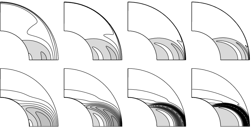
Figure 1: Contour plots of the angular velocity for $\epsilon=0$ (top row) and $\epsilon=1$ (bottom row). From left to right $Ha^{2}=10^{3}$, $10^{4}$, $10^{5}$ and $10^{6}$. $Re=E^{-1}=0$. Contour interval of 0.25, with super-rotating regions gray-shaded. The maximum values are 1.28, 1.32, 1.35 and 1.36 in the top row, and 1.71, 2.45, 3.89 and 6.54 in the bottom row.

The left panel in Fig. 2 quantifies how the super-rotation varies with $Ha$, for different values of $\epsilon$. For $\epsilon=1$ it does indeed appear to scale as $Ha^{1/2}$, as predicted by the asymptotic analysis [7]. Turning next to $\epsilon=0.1$, $10^{-2}$ and $10^{-3}$, we note that for sufficiently large $Ha$ even $\epsilon=10^{-3}$ deviates from $\epsilon=0$, and starts to rise. This would seem to confirm the suggestion made by [8] that the relevant ratio is not the boundary’s conductance compared with the conductance of the entire depth of fluid, but only with the conductance of the Hartmann boundary layer. The thickness of this layer scales as $Ha^{-1}$, suggesting that the relevant parameter is not $\epsilon$ itself, but rather $\epsilon\,Ha$. Once this exceeds $O(1)$, the boundary is qualitatively more like conducting than insulating. For any non-zero $\epsilon$ the degree of super-rotation should therefore eventually start to rise, just as seen here.

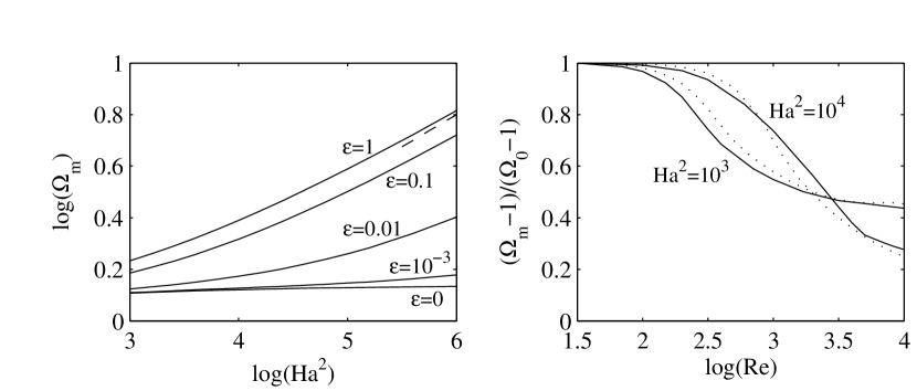
Figure 2: The left panel shows how the maximum value of the angular velocity varies with $Ha$, for the indicated values of $\epsilon$. The dashed line segment alongside the $\epsilon=1$ curve denotes the $Ha^{1/2}$ expected asymptotic scaling. The right panel shows how the quantity $(\Omega_{m}-1)/(\Omega_{0}-1)$ varies with $Re$, where $\Omega_{m}$ is the maximum value of the angular velocity at the given $Re$, and $\Omega_{0}$ is the maximum value of the angular velocity at $Re=0$. Solid lines are $\epsilon=1$, dotted lines are $\epsilon=0$, and Hartmann numbers as indicated.

All these results so far have been for $Re=0$, the infinitesimal differential rotation limit considered previously [3-7]. Figure 3 shows how the flow is altered if we now increase $Re$, to the point where inertial and magnetic effects are comparable (that is, $N=1$). We note first that in addition to the angular velocity, there is now a meridional circulation as well, which has a significant effect back on the angular velocity. In particular, the previous super-rotation on $\mathcal{C}$ is strongly suppressed, and also pushed inward, until there is nothing left of the original structure on $\mathcal{C}$. Another interesting feature to note is how the meridional circulation compresses the remaining outer boundary layer until it is much thinner than the original, linear boundary layer.

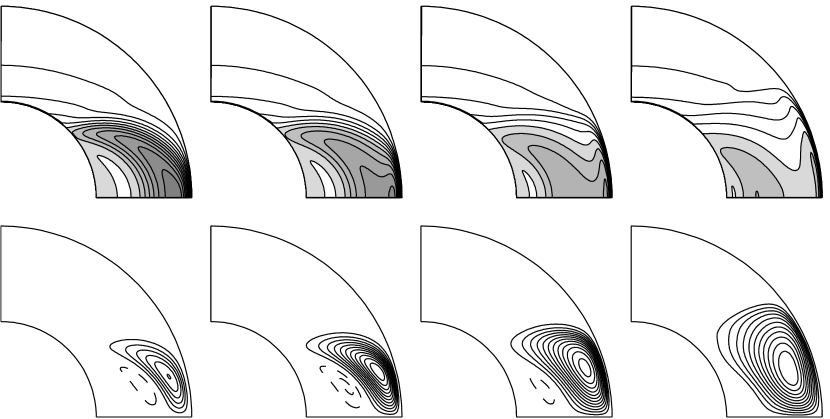
Figure 3: $Ha^{2}=10^{4}$, $E^{-1}=0$, $\epsilon=1$, and from left to right $Re=300$, 1000, 3000 and 10000. The top row shows contours of the angular velocity, with a contour interval of 0.2, and super-rotating regions gray-shaded. The bottom row shows streamlines of the meridional circulation, with solid lines denoting counter-clockwise circulation (with a contour interval of $10^{-3}$), and dashed lines denoting a much weaker clockwise circulation (with a contour interval of $5\cdot 10^{-4}$). The angular velocity is symmetric about the equator, the meridional circulation anti-symmetric. Perturbations of the opposite symmetry were introduced, but decayed away in every case.

This behavior is very different from that obtained for an axial rather than a dipole field, where the axisymmetric basic state is almost unaffected by increasingly large $Re$, right up to the onset of non-axisymmetric instabilities [8]. The difference is that for a uniform axial field the flow is correspondingly also largely independent of $z$. If $\bf U$ only depends on $s$ though (where $z,s,\phi$ are cylindrical coordinates), then so does $\bf U\cdot\nabla U$, which can therefore be balanced by $-\nabla p$. In contrast, for the non-uniform dipole field considered here, $\bf U$ clearly depends on both coordinates $r$ and $\theta$, so $\bf U\cdot\nabla U$ cannot so easily be balanced by $-\nabla p$, but instead fundamentally alters the flow, as we see in Fig. 3.

Returning to Fig. 2, the right panel quantifies the suppression of the super-rotation, showing how $(\Omega_{m}-1)/(\Omega_{0}-1)$ varies with $Re$, where $\Omega_{m}$ is again the maximum angular velocity, at the given $Re$, and $\Omega_{0}$ is the maximum angular velocity at $Re=0$. That is, this quantity measures the relative amount by which the original super-rotation has been suppressed. Solid lines denote $\epsilon=1$, dotted lines $\epsilon=0$. We see therefore that even though conducting versus insulating outer boundaries yield very different degrees of super-rotation, the relative extent to which it is suppressed by $Re$ is surprisingly similar.

Note also how larger Hartmann numbers require larger $Re$ before the super-rotation starts to get suppressed. For example, if we focus on how large $Re$ must be before the super-rotation is suppressed to 80% of its original value, we find that it must be some 3 times larger for $Ha^{2}=10^{4}$ than for $Ha^{2}=10^{3}$, perhaps suggesting an $Re\sim Ha$ scaling. If true, this would indicate that the interaction parameter $N$ is not in fact the most appropriate measure of magnetic versus inertial effects for this problem.

The last point to note in this panel of Fig. 2 is that while larger Hartmann numbers may also require larger Reynolds numbers before the super-rotation starts to get suppressed, for sufficiently large $Re$ it is actually suppressed more for larger $Ha$. In particular, this suggests that for $Ha=210$ and $Re\gtrsim 10^{5}$ it might be suppressed to perhaps no more than 10% of its original $Re=0$ value, which would be consistent with the experimental findings of no clearly detectable super-rotation at all. (However, we must remember also that what little super-rotation is left is no longer situated on $\mathcal{C}$, but is instead concentrated at the inner sphere, where the experiment currently cannot make measurements. Once further ultrasound transducers are installed to measure the flow closer to the inner sphere, according to our results here they should measure at least some slight super-rotation.)

Figure 4 shows the solution at $Ha^{2}=10^{3}$ and $Re=10^{4}$. In addition to the remaining slight super-rotation at the equator of the inner sphere, there is now a new feature, namely a time-dependence near the outer sphere. The outer boundary layer periodically breaks down in mid-latitudes into a series of small-scale ripples, with period 0.0060, or $120\,\Omega_{i}^{-1}$ on the rotational timescale. None of this time-dependence penetrates very far into the interior though. One possible explanation for this is simply the $r^{-3}$ dipole field strength, which increases so strongly going inward that the interior is still magnetically dominated even at these values of $Re$.

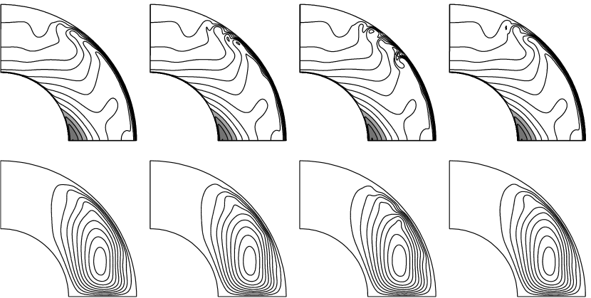
Figure 4: The solution at $Ha^{2}=10^{3}$, $Re=10^{4}$, $E^{-1}=0$, and $\epsilon=1$. From left to right four snapshots of the time-dependent solution, uniformly spaced throughout the period 0.0060, or $120\,\Omega_{i}^{-1}$. The top row shows contours of the angular velocity, with a contour interval of 0.1. The bottom row shows streamlines of the meridional circulation, with a contour interval of $10^{-3}$. Perturbations of the opposite equatorial symmetry were introduced, but decayed away.

Increasing $Re$ further, Fig. 5 shows the solution at $Re=15000$. The boundary layer eruptions are now considerably more pronounced, and cover a much broader range in latitude, including near the equator of the outer sphere. They are also no longer equatorially symmetric, but instead alternate between the two hemispheres. The period is 0.0014, or $42\,\Omega_{i}^{-1}$. This basic periodicity is quite regular, but the details of the individual pulses are not; the solution is evidently quasi-periodic.

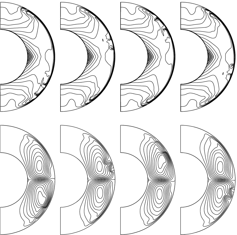
Figure 5: As in Fig. 4, but at $Re=15000$. The period is 0.0014, or $42\,\Omega_{i}^{-1}$. The numerical resolution was 135 Chebyshev polynomials in $r$ times 720 Legendre polynomials in $\theta$, and was checked to ensure that even these very fine structures are adequately resolved.

We note that the experiment also exhibits rapid fluctuations near the outer boundary, but a much more quiescent interior. To assess whether this might be related to our results here, we need to know how the critical Reynolds number for the onset of this time-dependence scales with $Ha$. Increasing $Re$ in steps of 200, we obtained $Re_{c}=9800$, 12600 and 16400, for $Ha^{2}=1000$, 2000 and 4000, respectively. The ratios 12600/9800=1.29 and 16400/12600=1.30 then suggest the scaling $Re_{c}\sim Ha^{0.74}$, although of course with only three data points, spanning a range of just 2 in $Ha$, one should not assign too much significance to this precise exponent 0.74. Nevertheless, it again demonstrates that the interaction parameter $N$ is not necessarily the most relevant ratio of Hartmann and Reynolds numbers. Furthermore, it suggests that the experiment should be far above the critical Reynolds number for the onset of this time-dependence, so the fluctuations observed in the experiment may indeed include these instabilities discovered here (in addition to possible non-axisymmetric instabilities not considered here).

It is interesting also to compare our $Re_{c}\approx 760Ha^{0.74}$ instabilities with the Hartmann layer instabilities explored by [10,11], who found that $Re_{c}\approx 380Ha$. Inserting our values of $Re_{c}$ and $Ha$, for $Ha^{2}=1000$, 2000 and 4000 we obtain $Re_{c}/Ha=310$, 280 and 260; sufficiently close to 380 that the instabilities are likely to be closely related. The slightly different scalings with $Ha$ could plausibly be explained by the fact that the spherical shell geometry considered here is considerably more complicated than the planar geometry considered by [10,11], and correspondingly our basic state depends on $Ha$ and $Re$ in a more complicated way than it does in planar geometry. See also [12], who consider Hartmann layer instabilities in a rather different parameter regime, appropriate to the Earth’s rapidly rotating core.

Finally, the last point to note is that $\epsilon=0$ yields solutions similar to Figs. 4 and 5, merely at somewhat larger values of $Re$. This is perhaps not surprising: the main effect of $\epsilon$ appears to be to control the degree of super-rotation, just as it did in the linear regime, but as Figs. 4 and 5 show, this time-dependence is completely unrelated to the remaining, rather weak super-rotation.

All results so far have been for $E^{-1}=0$, so a stationary outer sphere. In the experiment it was found that rotating the outer sphere tended to suppress these fluctuations near the outer boundary. We would therefore like to test whether adding an overall rotation will similarly suppress our instabilities in Figs. 4 and 5. But first, Fig. 6 shows the effect of adding a non-zero $E^{-1}$ to the previous solution in Fig. 3. Not surprisingly, an increasingly rapid overall rotation eventually suppresses all the previous structure, and the flow becomes almost completely aligned with the $z$-axis. Similar solutions were also obtained by [13], but coming from a rather different direction in parameter space, namely starting with a rapid rotation, and seeing how an increasingly strong magnetic field suppresses the so-called Stewartson layer on the tangent cylinder.

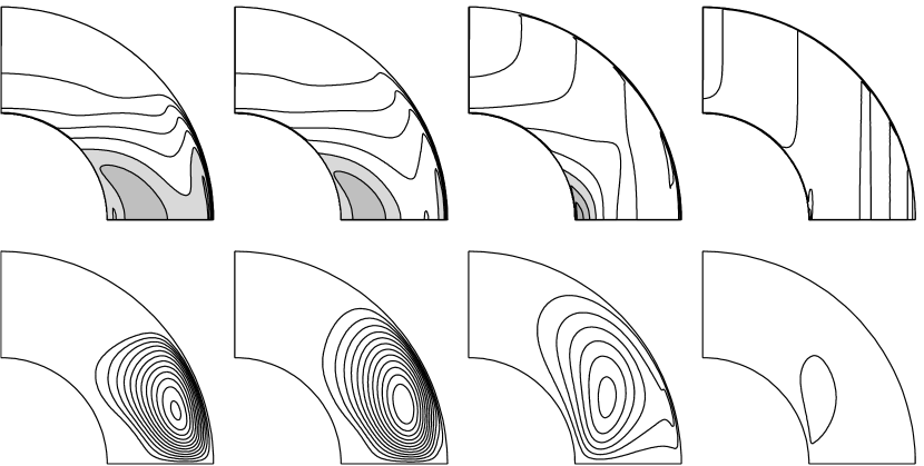
Figure 6: $Ha^{2}=10^{4}$, $Re=10^{4}$, $\epsilon=1$, and from left to right $E^{-1}=10^{3}$, $10^{4}$, $10^{5}$ and $10^{6}$. The top row shows contours of the angular velocity, with a contour interval of 0.2; the bottom row shows streamlines of the meridional circulation, with a contour interval of $10^{-3}$.

Given how effectively the Coriolis force suppresses the previous structure, it seems likely that it will also suppress the instabilities. Figure 7 shows that this is indeed the case; one can increase $Re$ up to 25000 at least, and still finds nothing like the instabilities in Figs. 4 and 5. One other interesting point to note regarding Figs. 6 and 7 is that the $Ha^{2}=10^{4},\ E^{-1}=10^{5}$ and $Ha^{2}=10^{3},\ E^{-1}=10^{4}$ solutions look rather similar, and similarly $E^{-1}=10^{6}$ and $E^{-1}=10^{5}$. This indicates that, unlike the interaction parameter $N$, the Elsasser number $\Lambda=Ha^{2}E$ is indeed the relevant parameter here.

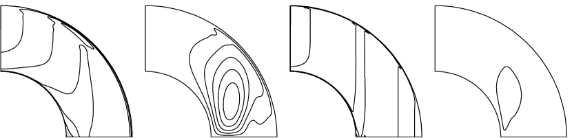
Figure 7: $Ha^{2}=10^{3}$, $Re=25000$, $\epsilon=1$. The first two panels show the angular velocity and meridional circulation at $E^{-1}=10^{4}$, the second two panels at $E^{-1}=10^{5}$. Contour intervals again 0.2 and $10^{-3}$.

4 Conclusion

We have found that the inclusion of inertia in this magnetic spherical Couette flow problem radically alters the results, suppressing the previous super-rotation, and completely eliminating the significance of the field line $\mathcal{C}$. For sufficiently large Reynolds numbers we also discovered instabilities in the outer boundary layer, which may be related to some of the fluctuations seen in the experiment, particularly as a rapid overall rotation suppresses them again in both the experiment and here.

Finally, there are (at least) two further issues that should be explored numerically. First, what about non-axisymmetric instabilities, for example Görtler vortices associated with the meridional circulation? It would certainly be of interest to compute critical Reynolds numbers for their onset, and see whether they are greater or smaller than the $Re_{c}\approx 760Ha^{0.74}$ onset of the axisymmetric instabilities considered here. The experiment did not show any large-scale non-axisymmetric structures, but was not purely axisymmetric either. This suggests that the most unstable non-axisymmetric modes may have very high azimuthal wavenumber $m$ (which would be consistent with small-scale Görtler vortices). If the 3D solutions exhibit structure in $\phi$ comparable to the structure in $\theta$ seen in Figs. 4 and 5, that would certainly correspond to very high $m$ indeed, making fully 3D solutions very difficult.

Second, we recall that all of our calculations were in the small $Rm$ limit (7,8). For the solutions here, this is appropriate, since $Re=25000$, the largest value considered, still corresponds to $Rm<1$. In the experiment though $Re$ is so large that even $Rm>1$. Furthermore, finite $Rm$ opens up the possibility of fundamentally new dynamics, such as the magnetorotational instability. It would be of considerable interest therefore to consider finite $Rm$, and see whether anything emerges that is completely different from the results presented here. Some of these calculations are currently under way.

References

- [1] P. Cardin, D. Brito, D. Jault, H.-C. Nataf, J.-P. Masson, Towards a rapidly rotating liquid sodium dynamo experiment, Magnetohydrodynamics 38 (2002) 177–189.
- [2] H.-C. Nataf, T. Alboussiere, D. Brito, P. Cardin, N. Gagniere, D. Jault, J.-P. Masson, D. Schmitt, Experimental study of super-rotation in a magnetostrophic spherical Couette flow, Geophys. Astrophys. Fluid Dynam. 100 (2006) 281–298.
- [3] S.V. Starchenko, Magnetohydrodynamic flow between insulating shells rotating in strong potential field, Phys. Fluids 10 (1998) 2412–2420.
- [4] E. Dormy, P. Cardin, D. Jault, MHD flow in a slightly differentially rotating spherical shell, with conducting inner core, in a dipolar magnetic field, Earth Planet. Sci. Lett. 160 (1998) 15–30.
- [5] E. Dormy, D. Jault, A.M. Soward, A super-rotating shear layer in magnetohydrodynamic spherical Couette flow, J. Fluid Mech. 452 (2002) 263–291.
- [6] R. Hollerbach, Magnetohydrodynamic flows in spherical shells, in Physics of Rotating Fluids (Editors C. Egbers, G. Pfister), Springer (2000) 295–316.
-
[7]
L. Buehler, On the origin of super-rotating tangential layers in
magneto- hydrodynamic flows,
http://bibliothek.fzk.de/zb/berichte/FZKA7028.pdf
(2004). - [8] R. Hollerbach, S. Skinner, Instabilities of magnetically induced shear layers and jets, Proc. R. Soc. Lond. A 457 (2001) 785–802.
- [9] R. Hollerbach, A spectral solution of the magneto-convection equations in spherical geometry, Int. J. Numer. Meth. Fluids 32 (2000) 773–797.
- [10] P. Moresco, T. Alboussiere, Experimental study of the instability of the Hartmann layer, J. Fluid Mech. 504 (2004) 167–181.
- [11] D.S. Krasnov, E. Zienicke, O. Zikanov, T. Boeck, A. Thess, Numerical study of the instability of the Hartmann layer, J. Fluid Mech. 504 (2004) 183–211.
- [12] B. Desjardins, E. Dormy, E. Grenier, Boundary layer instability at the top of the Earth’s outer core, J. Comp. Appl. Math. 166 (2004) 123–131.
- [13] R. Hollerbach, Magnetohydrodynamic Ekman and Stewartson layers in a rotating spherical shell, Proc. R. Soc. Lond. A 444 (1994) 333–346.