Observation of Kinetic Plasma Jets

Abstract

Under certain conditions an intense kinetic plasma jet is observed to emerge from the apex of laboratory simulations of coronal plasma loops. Analytic and numerical models show that these jets result from a particle orbit instability in a helical magnetic field whereby magnetic forces radially eject rather than confine ions with sufficiently large counter-current axial velocity.

Many lab and space plasmas (e.g., solar coronal loops Tandberg , spheromaks Bellan_book2000 , tokamaks Tokamak , and magnetic clouds Burlaga ) are presumed to be magnetic flux tubes filled with plasma confined via magnetohydrodynamic (MHD) forces. However, confinement can be significantly degraded in ways not predicted by MHD; e.g., in tokamaks, ions resulting from neutral beams injected against the toroidal current direction (counter-injection) exhibit severe orbit losses compared to co-injection Mikkelsen ; Egedal ; McClements . Related confinement degradation may be the cause of small solar corona jets (e.g., surges) associated with canceling magnetic features Chae ; Liu ; Harrison and of coronal streamers emanating from magnetic neutral lines Li . This Letter reports that in certain circumstances an ion injected along the axis of a magnetic flux tube will be magnetically ejected from the flux tube instead of being magnetically confined, i.e., the ion will have radially unstable motion (RUM). This instability explains the severe orbit losses of counter-injected ions in tokamaks and is likely relevant to similar situations occurring in the solar corona. The instability, labeled as ‘Kinetic Plasma Jet’ in Fig. 1, was discovered experimentally and then modeled.

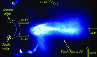
Figure 1: (Color online) Kinetic plasma jet emanating from an argon laboratory loop. Dashed arch corresponds to initial plasma loop at $t\approx 1.0$ $\mu$s as in Fig. 4(b). Arrows represent lines of sight (los#) used for spectroscopy; arrow widths represent $\sim 6$ mm diameter of lines of sight.

We first outline the physical basis for RUM. Consider a particle injected with velocity $v_{z0}$ near the axis of a cylindrical flux tube having helical magnetic field $\mathbf{B=}B_{\phi}\hat{\phi}+B_{z}\hat{z}.$ The flux tube geometry is sketched in Fig. 2(a) and corresponds to a straightened-out model of Fig. 2(b), our laboratory configuration simulating a coronal loop Hansen04 . The $r$ component of $md\mathbf{v}/dt=q\mathbf{v\times B}$ is $m\ddot{r}-mr\dot{\phi}^{2}=qr\dot{\phi}B_{z}-qv_{z}B_{\phi}$. If $v_{z}B_{\phi}=0$, then radial force balance $\ddot{r}=0$ gives $\dot{\phi}=-qB_{z}/m=-\omega_{c}$, i.e., the conventional cyclotron orbit. However, if $v_{z}B_{\phi}\neq 0$, then radial force-balance $\ddot{r}=0$ requires $\dot{\phi}^{2}+\dot{\phi}qB_{z}/m-v_{z}qB_{\phi}/mr=0$ so no real $\dot{\phi}$ solutions exist if

$$B_{z}^{2}+4mv_{z}B_{\phi}/qr<0.$$ (1)

Thus, large negative $mv_{z}B_{\phi}/qr$ causes the radially outward force$\ -qv_{z}B_{\phi}$ to overwhelm the radially inward force $qr\dot{\phi}B_{z}$ so centrifugal force $mr\dot{\phi}^{2}$ is unbalanced.

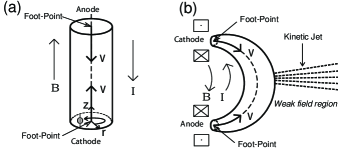
Figure 2: (a) Flux tube geometry used in the model. (b) Experimental configuration; $B$ outside the flux loop is weakest on the right hand side (indicated as weak field region).

We next use Hamiltonian arguments to show that satisfying Eq. (1) leads to the particle being radially ejected from the flux tube, i.e., RUM. In order to model the simplest nontrivial situation, both $B_{z}$ and the axial current density $J_{z}$ are assumed uniform within the flux tube so in the flux tube the vector potential is $\mathbf{A}(r)=\hat{\phi}B_{z}r/2-\hat{z}\mu_{0}J_{z}r^{2}/4,$ the axial flux is $\Phi=B_{z}\pi r^{2},$ and the axial current is $I=J_{z}\pi r^{2}.$ Using the Lagrangian $L=m(v_{r}^{2}+r^{2}\dot{\phi}^{2}+v_{z}^{2})/2+qr\dot{\phi}A_{\phi}+qv_{z}A_{z}$, the canonical momenta $P_{\phi}=\partial L/\partial\dot{\phi}$ and $P_{z}=\partial L/\partial v_{z}$ are

$$P_{\phi}=\ mr^{2}\dot{\phi}+qr^{2}B_{z}/2,\text{ \ }P_{z}=mv_{z}-\mu_{0}qJ_{z}r^{2}/4.$$ (2)

Because $\phi$ and $z$ are ignorable, both $P_{\phi}$ and $P_{z}$ are invariants. A particle injected with velocity $v_{z0}$ along the the flux tube axis (i.e., at $r=0)$ thus has the invariants

$$P_{\phi}=0\text{, \ \ }P_{z}=mv_{z0}.$$ (3)

Combining Eqs. (2) and (3) gives $\dot{\phi}=-\omega_{c}/2$ and $v_{z}=v_{z0}+\omega_{c}r^{2}\lambda/4$ where    $\lambda=\mu_{0}J_{z}/B_{z}=\mu_{0}I/\Phi$ is related to twist. The Hamiltonian $H=m(v_{r}^{2}+r^{2}\dot{\phi}^{2}+v_{z}^{2})/2$ can be expressed as $H=mv_{r}^{2}/2+f(r)$ where

$$f(r)=\frac{m\omega_{c}^{2}}{2\lambda^{2}}\left[\frac{\lambda^{2}r^{2}}{4}+\left(\frac{\lambda v_{z0}}{\omega_{c}}+\frac{\lambda^{2}r^{2}}{4}\right)^{2}\right]\$$ (4)

is an effective potential. On defining $\xi=\left|\lambda\right|r,$ the dimensionless effective potential $V(\xi)=2\lambda^{2}f(r)/m\omega_{c}^{2}$ can be written as

$$V(\xi)=\xi^{2}/4+\left(\lambda v_{z0}/\omega_{c}+\xi^{2}/4\right)^{2}.$$ (5)

Equation (5) gives $\partial V/\partial\xi=\xi/2+\lambda v_{z0}\xi/\omega_{c}+\xi^{3}/4$. Near the flux tube axis the $\xi^{3}/4$ term is negligible, so negative $\partial V/\partial\xi$ near the axis corresponds to having

$$S=\lambda v_{z0}/\omega_{c}+0.5<0.$$ (6)

Our main result is that if $S<0$ so $\partial V/\partial\xi<0$ near the axis, a particle at $r=0$ is on an effective potential hill as shown in the $S=-0.5$ curve in Fig. 3(a) and will fall radially out of the flux tube, i.e., RUM. Since $\lambda=2B_{\phi}/B_{z}r$, Eq. (6) is identical to Eq. (1). All magnetic flux tubes have uniform $B_{z}$ and $J_{z}$ near the axis so particles with $S<0$ will always be on a potential hill and experience RUM. Equation (6) can be written in terms of experimental parameters as

$$S=KIv_{z0}/q+0.5<0$$ (7)

where $K=\mu_{0}\pi mr^{2}/\Phi^{2}$   is positive, showing that RUM requires $Iv_{z0}/q<0$, i.e., counter-current flow. Because $K\propto m$, ions have a much lower threshold for RUM than electrons.

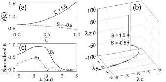
Figure 3: (a) $S=1.5$ gives ‘valley’ (i.e., stable) effective potential $V(\xi)$ while $S=-0.5$ gives    ‘hill’ (i.e., unstable). (b) Numerically calculated particle trajectories. (c) Probe measurement of flux tube magnetic field showing that field is weak on right side as sketched in Fig. 2(b).

Figure 3(a) plots $V(\xi)$ given by Eq. (5) for $S=-0.5$ and $1.5$, while Fig. 3(b) plots trajectories calculated from direct numerical integration of $m\mathbf{\ddot{r}=}q\mathbf{v\times}\left(B_{\phi}\hat{\phi}+B_{z}\hat{z}\right)$ for a particle with $S=-0.5$ (i.e., $v_{z0}=-\omega_{c}/\lambda$) starting at the down arrow and for a particle with $S=1.5$ (i.e., $v_{z0}=+\omega_{c}/\lambda$) starting at the up arrow. Injection at $\lambda x=\lambda y=10^{-6}$ is used so a particle does not start exactly at the top of a potential hill. To approximate the weak field to the right of the flux loop sketched in Fig. 2(b), an exponentially decaying $B_{z}$ in the current-free external region is used in the numerical calculation. Figure 3(b) shows that the $S=-0.5$ particle is ejected from the flux tube (i.e., RUM), whereas the $S=1.5$ particle remains on the flux tube axis (i.e., is confined).

Our experimental configuration Hansen04 , sketched in Fig. 2(b), involves top and bottom electrodes (respectively cathode and anode) mounted on the end dome of a large vacuum chamber (base pressure $\sim 10^{-7}$ mbar). The experimental sequence is: (i) slow ($\sim 10$ ms) electromagnets behind the electrodes create an initial arched vacuum magnetic field, (ii) a fast ($\sim 1$ ms) gas valve injects neutral gas from orifices in the electrodes, (iii) a $\sim 1$ kJ, 59 $\mu$F capacitor switched across the electrodes breaks down the neutral gas, (iv) a bright plasma loop appears. The 10–20 $\mu$s dynamical evolution of this loop is imaged EPAPS by a fast digital framing camera. Detailed measurements in a similar experiment You showed that the bulk plasma in the flux loop is many orders of magnitude denser than the injected pre-breakdown neutral gas and results from fast MHD ingestion into the loop of orifice-originating plasma Bellan05 . Figure 3(c) shows magnetic probe Romero measurements of flux tube $B_{\phi}$ and $B_{z}$ as functions of distance $L$ from the flux tube axis in the direction away from the electrode plane (data deconvolved as in Ref. Burlaga ); the magnetic field amplitude decays rapidly to the right (corresponding to weak field region in Fig. 2(b)).

Figure 4 shows the evolution of Ar plasma loops for different injected gas mass $M_{n}$ and different flux $\Phi$ as a function of time measured from breakdown. $M_{n}$ was determined using a thermocouple gauge and has only a relative meaning because the plasma shot, being much shorter than the gas puff time, uses only a fraction of $M_{n}$. Since the plasma has very low impedance, the capacitor acts approximately as a current source. This is consistent with the observation that $I$ and hence $\lambda/\omega_{c}$ are essentially unaffected when $M_{n}$ is varied. However, the plasma velocity $v_{z0}$ is observed to be strongly dependent on $M_{n}$ with higher $v_{z0}$ observed at smaller $M_{n}$.

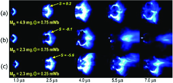
Figure 4: (Color online) Evolution of laboratory plasma loops at (a) high $M_{n}$, (b) low $M_{n}$, and (c) low $\Phi$. Movies placed in Ref. EPAPS show the evolutions even more dramatically.

Figure 4(a) corresponds to $M_{n}=4.9$ mg, $\Phi=0.75$ mWb; Fig. 4(b) to $M_{n}=2.3$ mg, $\Phi=0.75$ mWb; and Fig. 4(c) to $M_{n}=2.3$ mg, $\Phi=0.25$ mWb. In the first two frames of Figs. 4(a-c) the plasma has a smooth arch shape; $I$ is low at this stage and the plasma follows the half-torus profile of the initial vacuum magnetic field spanning the electrodes. Then, as $I$ increases, the plasma minor radius decreases due to self-pinching while the major radius increases due to the hoop force Hansen01 associated with the poloidal magnetic field produced by $I$. While this is happening, the loop undergoes MHD kink instability and the projection of the writhed loop axis results in a cusp-like dip at the apex Hansen01 . In the second frame (i.e., $2.5$ $\mu$s) of Figs. 4(a,b) a finger-like stream of plasma emerges near the top (i.e., near cathode) of the loops. In Fig. 4(b), which corresponds to low $M_{n}$ and hence high $v_{z0}$, the stream moves toward the ground plane near the cathode and leads to a major disruption in $I$. As also seen in Fig. 4(b), this is followed by the detachment of the loop from the electrodes and, for $t>4$ $\mu$s, formation of a plasma jet propagating far to the right of the electrodes (see also Fig. 1) into the weak field region (i.e., to the right in Figs. 2(b) and 3(c)). A significant drop in $I$ is observed during the detachment phase as well as an associated upward voltage spike. From this time on, $I$ commutates to a new shorter path between the electrodes, while the detached plasma jet propagates away from the electrodes. When $\Phi$ is lowered as shown in Fig. 4(c), two critical stages of the detachment are clearly seen in the 4.0–7.0 $\mu$s frames, specifically the loop first detaches from the cathode and then from the anode to form an intense plasma jet. Figures 4(a-c) also display $S$ estimated using measured cathode region quantities in Eq. (7) at 2.5 $\mu$s (i.e., just before detachment) and indicate that the plasma jet development in Figs. 4(b, c) is associated with having $S<0$.

Equation (7) shows that only ions with $v_{z0}$ being large and negative relative to $I$ can have $S<0$. Measurements (discussed below) indicate that near the cathode ions with large negative $v_{z0}$ ($\sim 40$–$60$ km/s) indeed exist. The slowing-down time ($>100~{}\mu$s) of these fast ions by the plasma (density $\sim 10^{20}$ m^-3) is much longer than the plasma duration, therefore collisions cannot affect their orbits. Since the ion contribution to electric current necessarily flows in the same direction as the current, ion drift motion associated with electric current cannot account for the observed large negative $v_{z0}$. Furthermore, because the measured $\left|v_{z0}\right|$ greatly exceeds the Ar⁺ thermal speed $v_{T}\sim$2–5 km/s estimated using the spectroscopically determined $T_{i}\sim$1–10 eV, neither can ion thermal motion account for the observed large negative $v_{z0}.$ However, there does exist a mechanism capable of accelerating ions to high velocities either parallel or anti-parallel to $I$. This mechanism Bellan05 ; You shows that axial gradients of $B_{\phi}^{2}$ provide an MHD force $\sim-\partial B_{\phi}^{2}/\partial z$ that accelerates plasma from regions of large $B_{\phi}^{2}$ to regions of small $B_{\phi}^{2}$, i.e., acceleration occurs from both foot-points of a flux loop towards the apex if the flux loop minor radius is smaller at the foot-points than at the apex (see detailed discussion in Ref. Bellan05 ). The resulting velocity is $v_{z}\sim B_{\phi}/\sqrt{\mu_{0}m_{i}n_{i}}$, consistent with higher ion axial velocity observed at smaller neutral gas injection pressures.

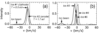
Figure 5: Measured spectra of an $\text{Ar}^{+}$ line (rest-frame wavelength $\lambda_{0}=434.806$ nm shown by vertical lines). Velocity is $v=c(\lambda-\lambda_{0})/\lambda_{0}$ where $\lambda$ is measurement wavelength, $c$ is speed of light. Lines of sight (los #) are shown in Fig. 1. (a) Spectra from the cathode (los #1) and anode  (los #2) regions for $t$ = 0–0.5 $\mu$s. (b) Spectra from the kinetic jet region along los #3, #4, and #5 for $t$ = 2.5–5.5 $\mu$s, 7.0–9.0 $\mu$s, and 6.0–18.0 $\mu$s respectively.

Ar⁺ Doppler velocity measurements have been made using a 1 m monochromator with a gated intensified CCD camera with fiber/lens coupling system. The spectra displayed in Fig. 5 show velocity components along lines of sight (los) indicated in Fig. 1 by “los #”. The los #1 and #2 spectra in Fig. 5(a) show that both cathode and anode emission lines are blue-shifted, confirming suprathermal ion flow from both cathode and anode towards the apex as predicted by Ref. Bellan05 . This outflow is seen in camera images as 30–60 km/s bright fronts propagating away from both electrodes along the flux loop axis towards its apex EPAPS . Figure 5(a) shows a large ion velocity component ($\sim 40$ km/s ion beam for los #1) moving away from the cathode while Fig. 5(b) shows spectra measured in the kinetic jet region and indicates a $\sim 50$ km/s ion beam for los #3. Because, as seen in Fig. 1, los #1 and los #3 make different angles relative to the respective flow directions being measured, ion beam velocities between different los #’s cannot be quantitatively compared, i.e., the $50$ km/s los #3 ion beam in Fig. 5(b) cannot be interpreted as a 10 km/s acceleration of the 40 km/s los #1 ion beam in Fig. 5(a).

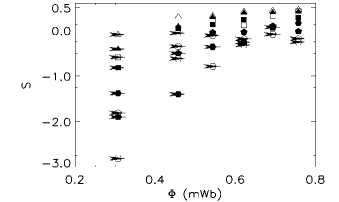
Figure 6: Measured $S$ for various plasma configurations. Filled/open symbols represent high/low $M_{n}$ respectively, number of sides in symbols represent capacitor charging voltage in kV, and arrow heads indicate plasma shots where kinetic jets are observed. Existence of kinetic jets has an excellent correlation with $S$ being negative.

Figure 6 shows the results of a parameter scan of $I,\Phi,$ and $v_{z0}$ performed to determine the $S$ dependence of the instability onset. $v_{z0}$ is determined from plasma front motion in the camera images EPAPS . The $S$ values in Fig. 6 were calculated using cathode region parameters in Eq. (7) for a large number of argon plasma loops ($r\simeq 8$ mm); $S=0.5$ is the upper bound for the observed negative $Iv_{z0}$. Kinetic jet instability, shown by arrow-heads in Fig. 6, occurs only when $S<0$ indicating excellent agreement with the RUM onset prediction.

The plasma loops used for Fig. 6 have already undergone MHD kink instability Hsu since all have $\left|\lambda\right|>4\pi/L\simeq 60$ m^-1, where $L\simeq$ 0.2 m is the loop length. The loops produce kinetic jets only when $S<0$ showing that RUM is a kinetic, rather than MHD, instability. The kinetic nature is also evident from the high velocity beams in Fig. 5 and from the kinetic jet appearing in the weak field (non-MHD) region as sketched in Fig. 2(b).

The RUM model explains why counter-injected neutral beams in tokamaks have severe orbit losses compared to co-injected neutral beams Mikkelsen ; Egedal ; McClements . In particular, Fig. 10 of Ref. Mikkelsen showed that an 80 keV counter-injected deuterium beam has severe orbit losses in a $B=0.3$ T tokamak having safety factor $q=1.25$ and major radius $R\simeq 1$ m. Since $\lambda\simeq 2/qR\simeq 1.6$ m${}^{-1},$ $\omega_{cD}=\allowbreak 1.\,\allowbreak 4\times 10^{7}$ s${}^{-1},$ and the injection velocity is $v_{inj}\ =\allowbreak 2.\,\allowbreak 8\times 10^{6}$ m/s, it is seen that $S_{counter}\simeq 0.5-\lambda v_{inj}/\omega_{cD}\ \approx 0.2$ whereas $S_{co}=0.5+\lambda v_{inj}/\omega_{cD}=0.8$; so, counter-injected ions have much larger orbits (i.e., broader valley-type effective potential as in Fig. 3(a)) than co-injected ions. While coronal loops are unlikely to have $S<0$ due to their small $\lambda$ ($\sim 10^{-8}$ m^-1) Burnette , jets associated with canceling magnetic features Chae ; Liu ; Harrison and coronal streamers Li emanating near magnetic neutral lines are both produced in extremely low magnetic field regions where $S<0$ could occur and RUM may be operative.

In summary, an instability has been demonstrated where ions are magnetically ejected from a flux tube. Ejection occurs when ions move opposite to the current with a sufficiently large axial velocity. We thank A. H. Boozer for pointing out a relationship between RUM and neutral beam counter-injection and D. Felt for technical assistance. Supported by US DOE and by NSF.

References

- (1) E. Tandberg-Hanssen, The Nature of Solar Prominences (Kluwer Academic, Dordrecht, 1995).
- (2) P. M. Bellan, Spheromaks (Imperial College Press, London, 2000).
- (3) J. Sheffield, Rev. Mod. Phys. 66, 1015 (1994).
- (4) L. F. Burlaga, J. Geophys. Res. 93, 7217 (1988).
- (5) D. R. Mikkelsen et al., Phys. Plasmas 4, 3667 (1997).
- (6) J. Egedal et al., Phys. Plasmas 10, 2372 (2003).
- (7) K. G. McClements and A. Thyagaraja, Phys. Plasmas 13, 042503 (2006).
- (8) J. Chae, Astrophys. J. 584, 1084 (2003).
- (9) Y. Liu and H. Kurokawa, Astrophys. J., 610, 1136 (2004).
- (10) R. A. Harrison, P. Bryans, and R. Bingham, Astron. Astrophys. 379, 324 (2001).
- (11) J. Li et al., Astrophys. J. 506, 431 (1998).
- (12) J. F. Hansen, S. K. P. Tripathi, and P. M. Bellan, Phys. Plasmas 11, 3177 (2004).
- (13) See EPAPS Document No. for movies and camera measurement example.
- (14) S. You, G. S. Yun, and P. M. Bellan, Phys. Rev. Lett. 95, 45002 (2005).
- (15) P. M. Bellan, Phys. Plasmas 10, 1999 (2003).
- (16) C. A. Romero-Talamas, P. M. Bellan, and S. C. Hsu, Rev. Sci. Instrum. 75, 2664 (2004).
- (17) J. F. Hansen and P. M. Bellan, Astrophys. J. 563, L183 (2001).
- (18) S. C. Hsu and P. M. Bellan, Phys. Rev. Lett. 90, 215002 (2003).
- (19) A. B. Burnette and R. C. Canfield, Astrophys. J. 606, 565 (2004).