QED calculation of the $2p_{3/2}-2p_{1/2}$ transition energy in five-electron ion of argon

Abstract

We perform ab initio QED calculation of the $(1s)^{2}(2s)^{2}2p_{3/2}$ - $(1s)^{2}(2s)^{2}2p_{1/2}$ transition energy in the five-electron ion of argon. The calculation is carried out by perturbation theory starting with an effective screening potential approximation. Four different types of the screening potentials are considered. The rigorous QED calculations of the two lowest-order QED and electron-correlation effects are combined with approximate evaluations of the third- and higher-order electron-correlation contributions. The theoretical value for the wavelength obtained amounts to 441.261(70) (nm, air) and perfectly agrees with the experimental one, 441.2559(1) (nm, air).

In the recent paper draganic:03 , high precision measurements of the $2p_{3/2}-2p_{1/2}$ transition energy in Ar XV, Ar XIV, Ar XI, and Ar X have been reported. The best results have been achieved for the five-electron ion of argon, where the experimental precision is 2700 times better than the theoretical one and 200 times better than that in the best of the previous measurements. This unprecedent precision provides a unique possibility to test various branches of the theory describing many-electron systems.

Since within the framework of the non-relativistic theory the $2p_{3/2}$ and $2p_{1/2}$ levels are degenerate, the transition energy is exclusively determined by the relativistic and quantum electrodynamic (QED) effects. Hence, investigation of this transition allows us to test the many-electron QED effects as well as calculations of the relativistic electron-correlation effects up to an extremely high level of accuracy.

To date ab initio calculations of many-electron QED effects were considered for two- and three-electron ions artemyev:05 ; yerokhin:01:pra2p . For systems with a larger number of electrons these effects were accounted for only within some one-electron or semi-empirical approximations safronova:96 ; draganic:03 ; indelicato:05 . Although the agreement of the results of Refs. draganic:03 ; indelicato:05 with experiment is rather good, the precision of these calculations is much worse compared to the experimental one. The improvement of this precision is a challenging problem for the theory. The goal of the present letter is to improve the theoretical precision for the $2p_{3/2}-2p_{1/2}$ transition energy in Ar¹³⁺. To achieve this goal we perform rigorous QED calculations to first two orders of perturbation theory and extremely large-scale configuration-interaction Dirac-Fock-Sturm (CI-DFS) calculations of the third- and higher-order contributions within the Breit approximation.

To formulate the QED perturbation theory we use the two-time Green function method shabaev:02:rep . Instead of usual Furry picture, where only the nucleus is considered as a source of the external field, we have used an extended version of the Furry picture. It implies incorporation of some screening potential, which partly accounts for the interelectronic interaction, into the zeroth-order Hamiltonian. The perturbation theory is formulated in powers of the difference between the full QED interaction Hamiltonian and the screening potential. This accelerates the convergence of the perturbative series. In addition, the usage of the screening potential allows us to avoid the degeneracy of the $(1s)^{2}(2s)^{2}2p_{3/2}$ and $(1s)^{2}(2p_{1/2})^{2}2p_{3/2}$ states that occurs if the pure Coulomb potential is employed as the zeroth-order approximation.

In the present letter we use four different types of the effective potential. The simplest choice is the core-Hartree (CH) potential. To obtain this potential we add the radial charge density distribution of the (four) core electrons

$$\rho_{\rm c}=2\sum_{n=1s,2s}(g_{n}^{2}+f_{n}^{2})$$ (1)

with $g$ and $f$ being the upper and lower radial components of the one-electron Dirac wave function to the radial charge density distribution $\rho_{\rm nuc}$ of the nucleus. The nuclear charge density is described by a Fermi distribution. The potential $V_{\rm CH}$ generated by the total charge density $\rho=\rho_{\rm nuc}+\rho_{\rm c}$ is calculated self-consistently by solving the Dirac equation.

The second choice is a local potential derived by inversion of the radial Dirac equation with the wave function obtained by solving the Dirac-Fock (DF) equation shabaev:05:pnc . We will refer to this potential as local Dirac-Fock (LDF) potential. The construction of the potential $V_{\rm LDF}$ is described in details in Ref. shabaev:05:pnc .

The other two potentials are based on the results of the density-functional theory (DFT). The first one is referred to as the Slater potential slater:51 . This potential belongs to the wide family of $x_{\alpha}$ potentials. Introducing the total one-electron radial density $\rho_{\rm t}$ via

$$\rho_{\rm t}(r) = 4\pi r^{2}\rho(r)\,,$$ (2)

$$\int\rho(r)d^{3}r = \int_{0}^{\infty}\rho_{\rm t}(r)dr=N\,,$$ (3)

where $N$ is the total number of the electrons, one can write the $x_{\alpha}$ potential in simple form:

$$V(r)=V_{\rm nuc}(r)+\alpha\int_{0}^{\infty}\frac{\rho_{\rm t}(r)}{r_{>}}-x_{\alpha}\frac{\alpha}{r}\left(\frac{81}{32\pi^{2}}r\rho_{\rm t}(r)\right)^{1/3}\,.$$ (4)

Here $\rho_{\rm t}$ denotes the total one-electron density, i.e. includes both core-electron and valence-electron density, while the CH potential includes only the core-electron density. The value of the constant $x_{\alpha}$ for the case of the Slater potential is equal to $1$. To improve the asymptotic behavior of this potential at large distances, a self-interaction correction, known also as the Latter correction latter:55 , has been added to it.

The fourth potential used in our calculations is known as Perdew-Zunger potential $V_{\rm PZ}$. It was constructed as described in Ref. perdew:81 .

The calculations of the transition energy can be conveniently divided in several steps. At first one has to solve the Dirac equation with the effective potential. Bound-state QED calculations require the representation of the quasi-complete set of the Dirac equation solutions. This was achieved by employing the dual-kinetic-balance (DKB) finite basis set method shabaev:04:dkb with basis functions constructed from B-splines johnson:88 .

Next we calculate the set of Feynman diagrams shown in Fig. 1 without any photon or electron loop, i.e. the part describing the interelectronic interaction. The dashed line ending with a triangle represents the interaction with the screening potential, taken with the opposite sign. The formulas for the calculations of the diagrams (a)-(d) in the framework of QED can be found in our previous works (see, e.g., Ref. yerokhin:01:pra2p ) devoted to the calculations of the two-photon exchange corrections to the energy levels of Li-like ions. We note that the diagrams containing only core electrons as initial (final) states can be omitted, because their contributions do not affect the transition energy. The formulas from Ref. yerokhin:01:pra2p in our case should be completed by similar ones with the $1s$ state being replaced by the $2s$ state. For the contributions of the diagrams (e)-(g) one can obtain:

$$\Delta E_{e} = V_{vv}\,,$$ (5)

$$\Delta E_{f} = \sum_{n\neq v}\frac{V_{vn}^{2}}{\varepsilon_{v}-\varepsilon_{n}}\,,$$ (6)

$$\Delta E_{g} = 2\sum_{c=1s,2s;\mu_{c}}\left[\sum_{n\neq v}\sum_{P}(-1)^{P}\frac{I_{PcPvcn}(\varepsilon_{Pc}-\varepsilon_{c})V_{nv}}{\varepsilon_{v}-\varepsilon_{n}}\right.$$ (7)

$$+\left.\sum_{n\neq c}\sum_{P}(-1)^{P}\frac{I_{PcPvnv}(\varepsilon_{Pv}-\varepsilon_{v})V_{nc}}{\varepsilon_{c}-\varepsilon_{n}}\right]$$

$$-\sum_{n=c}(V_{vv}-V_{nn})I^{\prime}_{vnnv}(\varepsilon_{v}-\varepsilon_{n})\,,$$

where $V_{ab}=-\langle a|V_{\rm scr}|b\rangle$, $I_{abcd}(\omega)=\langle ab|I(\omega)|cd\rangle$, $I(\omega)=e^{2}\alpha^{\mu}\alpha^{\nu}D_{\mu\nu}(\omega)$, $D$ is the photon propagator, $P$ is the permutation operator, $(-1)^{P}$ is the sign of the permutation, $I^{\prime}_{abcd}(\omega)=\langle ab|\frac{\partial}{\partial\omega}I(\omega)|cd\rangle$, and the indices $c$ and $v$ denote the wave functions of the core ($1s$ or $2s$) and the valence state, respectively.

In the next step we should take into account the contribution of the diagrams depicted in Fig. 2. The evaluation of the one-electron QED corrections of order $\alpha$, i.e. the self energy (SE) and the vacuum polarization (VP) (part (a) and (f) in Fig. 2) in an external Coulomb field is well known mohr:74 ; soff:88:vp ; manakov:89:zhetp ; mps:98 . High precision calculation of these diagrams for the case of an arbitrary external field, however, is a more involved problem cheng:93 ; lindgren:93:pra . We adopted the finite basis method for such calculations.

The main QED contribution to the energy of the forbidden transition arises from the one-electron SE diagram. To reach the required precision, this contribution has to be evaluated with at least 0.1% of accuracy. With this purpose, we decompose the SE diagram into zero-, one-, two-, and many-potential terms, as indicated in Fig. 3, where the dashed line ended with a cross denotes the full effective external potential. The zero- and one-potential terms have been calculated in momentum-space representation using the traditional renormalization scheme. The two-potential term has been evaluated in the coordinate space employing the analytical representation of the partial-wave decomposition of the free-electron Green function. To reach the required accuracy necessitates to sum over partial waves up to angular quantum number $\kappa=50$. Corresponding calculation within the B-spline approach would require an enormously large number of the basis functions, which would slow-down the computation considerably. To circumvent this problem we extracted the slowly-converging two-potential term and calculated it separately. A new numerical technique was elaborated for performing this calculation and will be described in details in our following work. The remaining many-potential term, containing three and more potentials, has been calculated within the DKB approach as the difference between the term, containing two- and more potentials and the two-potential one. The convergence of the partial-wave series for this term is very fast and, to reach the required accuracy, the summation can be restricted to $|\kappa|\leq 10$.

Since the contribution of the diagrams involving VP loops (parts (f–j) of Fig. 2) was found to be very small, we calculated it within the Uehling approximation. The total VP contribution to the transition energy in the Uehling approximation is about 0.2 cm^-1. The remaining Wichmann-Kroll contribution is negligible.

The other diagrams in Fig. 2 (b–e) represent the self-energy screening contributions. The irreducible part of the diagrams (d) and (e) can be calculated as a wave function correction to the one-electron SE diagram. This part was calculated using the same algorithm as it was used for the calculations of the one-electron SE diagram. The diagrams (b) and (c) are known as vertex diagrams. They were calculated in the traditional way: The bound-electron propagator was decomposed into zero- and many-potential terms. The zero-potential term is ultraviolet divergent. It was renormalized and calculated in momentum space together with the zero-potential term of the reducible part of the diagrams (d) and (e). The remaining many-potential term contains infrared divergent terms. These divergences are canceled by the infrared divergences in the reducible part of the many-potential term of the diagrams (d) and (e) (see, e.g., Ref. yerokhin:99:scr ). All the many-potential terms were calculated using the DKB approach.

The contribution of the interelectronic-interaction diagrams of the third and higher orders has been evaluated within the Breit approximation using the CI-DFS method. Going beyond the calculation performed in Ref. draganic:03 , the basis set of the configuration state functions was significantly enlarged and the quadruple excitations were included. To separate out the contribution of the third- and higher-order diagrams from the total energy, the following algorithm has been used. First of all, the Hamiltonian of the CI-DFS calculations was decomposed into parts

$$H = H_{0}+\lambda V\,,$$ (8)

$$H_{0} = H_{\rm free}+V_{\rm nuc}+V_{\rm scr}\,,$$ (9)

$$V = V_{ee}-V_{\rm scr}\,,$$ (10)

where $H_{0}$ is the unperturbed (zero-order) Hamiltonian, $V_{\rm nuc}$ and $V_{ee}$ denote the operators of the electron-nucleus and electron-electron (Coulomb and Breit) interaction, respectively. $V$ defines a perturbation and $\lambda$ is a freely varying parameter. This representation allows us to perform the expansion of the energy $E$ in powers of $\lambda$

$$E(\lambda)=E^{(0)}+\lambda E^{(1)}+\lambda^{2}E^{(2)}+\lambda^{3}E^{(\geq 3)}(\lambda)\,.$$ (11)

It is easy to see that the coefficients $E^{(1)}$ and $E^{(2)}$ correspond to the first- and second-order diagrams depicted in Fig. 1, calculated within the Breit approximation. Utilizing the same basis set these coefficients have been evaluated in two different ways: via numerical differentiation of $E(\lambda)$ with respect to $\lambda$ evaluated at $\lambda=0$ and directly by means of perturbation theory. The term $E^{(\geq 3)}$ is then calculated as the difference between the total energy and the first three terms in Eq. (11) evaluated at $\lambda=1$. The uncertainty of the $E^{(\geq 3)}$ contribution obtained in this way is estimated to be about 3 cm^-1. The QED contributions of the third and higher orders, which are beyond the Breit approximation, have not yet been evaluated. We estimate the uncertainty due to these effects as $\pm 2$ cm^-1.

The contribution of the one-electron two-loop QED-radiative corrections is very small and can be estimated using the analytical $\alpha Z$-expansion reported in Ref. jentschura:05 . Finally, one has to take into account the nuclear recoil effect. The calculation of this effect to all orders in $\alpha Z$ was performed in our recent paper orts:06 , where the isotope shift of the forbidden transition energies in B- and Be-like argon has been investigated.

The results of our calculations are presented in Table 1. In the first line of the table the difference between the one-electron Dirac energies of $2p_{3/2}$ and $2p_{1/2}$ states, calculated for the different screening potentials, is given. In the second row we give the contribution of first-order diagrams from Fig. 1 (diagrams (a) and (e)). These diagrams are calculated in the rigorous framework of QED, i.e. taking into account the energy dependence of the photon propagator. In the third line the contribution of the diagrams of the second order from Fig. 1 calculated within the Breit approximation is given. In the fourth line we give the QED correction to this contribution, i.e. the difference between these diagrams evaluated within the rigorous QED approach and within the Breit approximation. In the fifth line we give the contribution of the interelectronic-interaction diagrams of the third and higher orders derived from the CI-DFS calculations as described above. The contribution of the first- and second-order diagrams from Fig. 2 are presented in the sixth and seventh lines, respectively. The uncertainty due to uncalculated third- and higher-order QED effects is presented in eighth line. The following lines compile the contribution of the two-loop one-electron QED and the nuclear recoil correction, respectively. Finally, in the last line we present the total values of the energy of the forbidden $2p_{3/2}-2p_{1/2}$ transition in B-like argon, calculated for the four different screening potentials. Averaging these values and accounting for the uncertainty due to the higher-order interelectronic-interaction and QED effects, we obtain $E_{\rm tot}=$22656.1(3.6)cm^-1. This value is four times more precise than that of Ref. draganic:03 : 22662(14)cm^-1. The improvement mainly results from the calculation of the second-order QED effects (lines 4 and 7 in the table) as well as from the much more elaborated CI-DFS calculations performed in this work. Converting our result to the wavelength in air with the aid of Ref. stone_inet , one can obtain 441.261(70) (nm, air), which perfectly agrees with the experimental result 441.2559(1) (nm, air) from Ref. draganic:03 . Further improvement of the theoretical value can be achieved by the reducing of the uncertainty of the CI-DFS calculations and computation of the QED diagrams of the third and higher orders.

Summarizing, in this work we have calculated the energy of the forbidden $2p_{3/2}-2p_{1/2}$ transition in the five-electron ion of argon. The calculation incorporates the rigorous treatment of the second-order many-electron QED effects and the large-scale CI-DFS calculations of the third- and higher-order electron-correlation effects. This is the first ab initio treatment of the five-electron system in framework of QED. Significant improvement of the agreement between theoretical and experimental data has been achieved.

This work was partly supported by RFBR grant No. 04-02-17574. A.N.A. acknowledges the support by INTAS YS grant No. 03-55-960 and by the ”Dynasty” foundation. V.M.S., I.I.T., and G.P. acknowledge the support by INTAS-GSI grant No. 06-1000012-8881. G.P. also acknowledges support from DFG and GSI.

Table 1: Various contributions to the energy of the forbidden transition in B-like argon and the total result (in cm^-1).

	$V_{\rm CH}$	$V_{\rm LDF}$	$V_{\rm PZ}$	$V_{\rm Sl}$
$E_{\rm Dirac}$	$24343.0$	$25276.8$	$24860.7$	$26482.6$
$E^{(1)}_{\rm int}$	$-1002.9$	$-2064.2$	$-1539.3$	$-3451.8$
$E^{(2)}_{\rm int,Breit}$	$-1428.4$	$-1215.4$	$-1091.8$	$-993.3$
$E^{(2)}_{\rm int,QED}$	$6.2$	$5.5$	$5.0$	$8.7$
$E^{(\geq 3)}_{\rm int,Breit}$	$694.0(3.0)$	$608.2(3.0)$	$376.0(3.0)$	$567.6(3.0)$
$E^{(1)}_{\rm QED}$	$47.9$	$49.9$	$48.9$	$52.5$
$E^{(2)}_{\rm QED}$	$-2.2$	$-5.4$	$-3.8$	$-8.2$
$E^{(\geq 3)}_{\rm QED}$	$\pm 2.0$	$\pm 2.0$	$\pm 2.0$	$\pm 2.0$
$E_{\rm two-loop}$	$-0.1(1)$	$-0.1(1)$	$-0.1(1)$	$-0.1(1)$
$E_{\rm recoil}$	$-0.6$	$-0.6$	$-0.6$	$-0.6$
$E_{\rm total}$	$22656.9$	$22654.8$	$22655.2$	$22657.4$

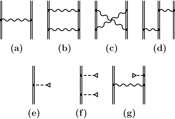
Figure 1: Interelectronic-interaction diagrams.

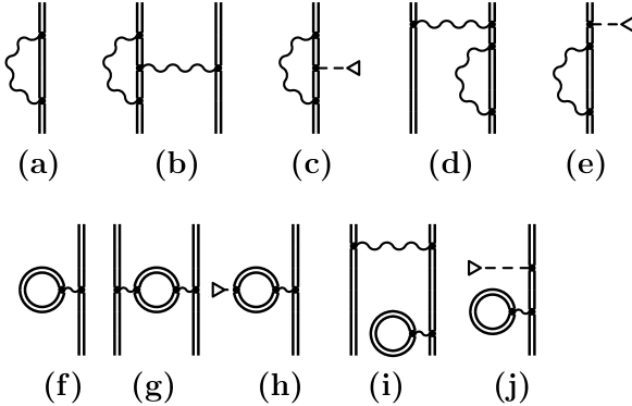
Figure 2: Self-energy and vacuum-polarization diagrams.

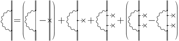
Figure 3: Diagram equation for the calculation of the one-electron self-energy contribution.

References

- (1) I. Draganić, J. R. Crespo López-Urrutia, R. DuBois, S. Fritzsche, V. M. Shabaev, R. Soria Orts, I. I. Tupitsyn, Y. Zou, and J. Ullrich, Phys. Rev. Lett. 91, 183001 (2003).
- (2) A. N. Artemyev, V. M. Shabaev, V. A. Yerokhin, G. Plunien, and G. Soff, Phys. Rev. A 71, 062104 (2005).
- (3) V. A. Yerokhin, A. N. Artemyev, V. M. Shabaev, M. M. Sysak, O. M. Zherebtsov, and G. Soff, Phys. Rev. A 64, 032109 (2001).
- (4) P. Indelicato, E. Lindroth, and J. P. Desclaux, Phys. Rev. Lett. 94, 013002 (2005).
- (5) M. S. Safronova, W. R. Johnson, and U. I. Safronova, Phys. Rev. A 54, 2850 (1996).
- (6) V. M. Shabaev, Physics Reports 356, 119 (2002).
- (7) V. M. Shabaev, I. I. Tupitsyn, K. Pachucki, G. Plunien, and V. A. Yerokhin, Phys. Rev. A 72, 062105 (2005).
- (8) J. C. Slater, Phys. Rev. 81, 385 (1951).
- (9) R. Latter, Phys. Rev. 99, 510 (1955).
- (10) J. P. Perdew and A. Zunger, Phys. Rev. B 23, 5048 (1981).
- (11) V. M. Shabaev, I. I. Tupitsyn, V. A. Yerokhin, G. Plunien, and G. Soff, Phys. Rev. Lett. 93, 130405 (2004).
- (12) W. R. Johnson, S. A. Blundell, and J. Sapirstein, Phys. Rev. A 37, 307 (1988).
- (13) P. J. Mohr, Ann. Phys. (New York) 88, 26, 52 (1974).
- (14) G. Soff and P. J. Mohr, Phys. Rev. A 38, 5066 (1988).
- (15) N. L. Manakov, A. A. Nekipelov, and A. G. Fainshtein, Zh. Eksp. Teor. Fiz. 95, 1167 (1989), [Sov. Phys. JETP 68, 673 (1989)].
- (16) P. J. Mohr, G. Plunien, and G. Soff, Phys. Rep. 293, 227 (1998).
- (17) K. T. Cheng, W. R. Johnson, and J. Sapirstein, Phys. Rev. A 47, 1817 (1993).
- (18) I. Lindgren, H. Persson, S. Salomonson, and A. Ynnerman, Phys. Rev. A 47, R4555 (1993).
- (19) V. A. Yerokhin, A. N. Artemyev, T. Beier, G. Plunien, V. M. Shabaev, and G. Soff, Phys. Rev. A 60, 3522 (1999).
- (20) U. D. Jentschura, A. Czarnecki, and K. Pachucki, Phys. Rev. A 72, 062102 (2005).
- (21) R. Soria Orts, Z. Harman, J. R. Crespo López-Urrutia, A. N. Artemyev, H. Bruhns, A. J. G. Martínez, U. D. Jentschura, C. H. Keitel, A. Lapierre, V. Mironov, V. M. Shabaev, H. Tawara, I. I. Tupitsyn, J. Ullrich, and A. V. Volotka, Phys. Rev. Lett. 97, 103002 (2006).
- (22) J. A. Stone and J. H. Zimmerman, http://emtoolbox.nist.gov .