Ionization of Sodium and Rubidium nS, nP and nD Rydberg atoms by blackbody radiation

Abstract

Results of theoretical calculations of ionization rates of Rb and Na Rydberg atoms by blackbody radiation (BBR) are presented. Calculations have been performed for nS, nP and nD states of Na and Rb, which are commonly used in a variety of experiments, at principal quantum numbers n=8-65 and at three ambient temperatures of 77, 300 and 600 K. A peculiarity of our calculations is that we take into account the contributions of BBR-induced redistribution of population between Rydberg states prior to photoionization and field ionization by extraction electric field pulses. The obtained results show that these phenomena affect both the magnitude of measured ionization rates and shapes of their dependences on n. The calculated ionization rates are compared with the results of our earlier measurements of BBR-induced ionization rates of Na nS and nD Rydberg states with n=8-20 at 300 K. A good agreement for all states except nS with $n>15$ is observed. We also present the useful analytical formulae for quick estimation of BBR ionization rates of Rydberg atoms.

I Introduction.

Blackbody radiation (BBR) is known to strongly affect the populations of atoms in highly excited Rydberg states Gallagher . It has also been shown that at the ambient temperature of 300 K BBR can photoionize Rydberg atoms with $n\sim 20$ at astonishingly high rates ($\sim 10^{3}\,\mathrm{s}^{-1}$) SpencerIon ; Beiting ; Spencer . Strong effect of BBR on Rydberg atoms is related to large matrix elements of bound-bound and bound-free transitions between Rydberg states in the microwave and far infrared spectral range Rydberg atoms .

Interaction of Rydberg atoms with BBR has been studied earlier in various contexts. Farley and Wing Farley calculated the dynamic Stark shifts and depopulation rates of Rydberg levels of alkali atoms with $n\leq 30$ at 300 K. The temperature dependence of BBR-induced transitions rates from the 19S state of sodium was calculated and measured by Spencer et al Spencer . Galvez et al Galvez1 ; Galvez2 have studied BBR-induced cascade transitions from the initially populated $n$=24-29 states of Na, both theoretically and experimentally.

Although interaction of Rydberg atoms with blackbody radiation has been studied for years, both theoretically and experimentally, only a few works were devoted to BBR-induced ionization of Rydberg atoms itself. The temperature dependence of the BBR-induced ionization rate of Na 17D state was numerically calculated using the quantum defect method in a Coulomb approximation and experimentally measured by Spencer et al SpencerIon . A simple scaling law for BBR ionization rates was also introduced in that work. More recently, the interest to BBR-induced ionization of Rydberg atoms has been related to the spontaneous formation of ultracold plasma in dense samples of cold Rydberg atoms Robinson ; Li , and to the prospects of its use as a convenient reference signal in absolute measurements of collisional ionization rates PaperI . Even nowadays, however, the studies of spontaneous evolution of ultracold Rydberg atoms to a plasma caused by BBR Robinson ; Li use the simple estimates of BBR ionization rates taken from the well-known work SpencerIon . The numerical calculations of direct BBR photoionization rates were performed by Lehman Lehman for H and Na Rydberg states with $n$=10-40 using a Herman-Skillman potential with an additional term to account for core polarization. However, the theoretical data for Rb atoms, which are widely investigated in experiments on ultracold plasma, are lacking. No systematic experimental studies of the $n$-dependences of BBR ionization rates of alkali-metal Rydberg atoms in a wide range of principal quantum numbers are known.

A major problem in the interpretation of measured ionization rates of Rydberg atoms is related to the fact that populations of Rydberg states are affected by BBR-induced processes to an unknown (or, at least, not straightforwardly predictable) extent, which depends on the combination of specific experimental conditions (principal quantum numbers n, ambient temperature, duration of measurements, extracting electric field strengths, etc.). Therefore, a more detailed study of BBR-induced ionization of Rydberg atoms under typical experimental conditions is required, especially for higher Rydberg states that are often explored in the experiments with cold atoms.

In this article we present the results of numerical calculations of BBR ionization rates of Rb and Na Rydberg atoms for the most commonly used nS, nP and nD states with n=8-65 at the ambient temperatures of 77, 300 and 600 K. In these calculations we take into account two phenomena that may affect the observed ionization rates: the time-dependent BBR-induced population redistribution between Rydberg states prior to photoionization and the selective field ionization (SFI) of high-lying Rydberg states by the electric field applied for extraction of ions from the excitation zone. Although both phenomena were mentioned in some of the earlier studies SpencerIon , their effects have not yet been studied in sufficient detail neither theoretically, nor experimentally. In particular, in the measurements of direct BBR photoionization rate of the sodium 17D state SpencerIon with effective lifetime 4 $\mu$s at the ambient temperature of 300 K, the effect of population redistribution was diminished due to the short measurement time of 500 ns and weak electric field used for extraction of ions. However, for Rydberg states with $n\sim 8$ and effective lifetimes less than 500 ns even this very short time interval is insufficient to avoid mixing with neighboring states, so that mixing processes must be necessarily accounted in calculations. In the present study we address to both phenomena and provide the useful analytical formulae, which can be applied to any Rydberg atom for estimates of the direct BBR-induced ionization rates and of the contribution of the SFI.

The simplest (but often insufficient) way of considering BBR-induced ionization after the excitation of an atom A to a given nL Rydberg state is to limit the problem to the direct photoionization of the initial nL state in one step by absorption of BBR photons:

$$A\left({nL}\right)+\hbar\omega_{BBR}\to A^{+}+e^{-},$$ (1)

where $\hbar\omega_{BBR}$ is the energy of absorbed BBR photon, $A^{+}$ is the atomic ion, and $e^{-}$ is the free electron emitted in the ionization. In the reality, however, ionization of Rydberg atoms exposed to BBR is a complex process, in which the following main components can be identified [see Fig. 1(a)]: (i) direct photoionization of atoms from the initial Rydberg state via absorption of BBR photons, (ii) field ionization by extraction electric field pulses of high Rydberg states, which are populated from the initial Rydberg state by absorption of BBR photons, (iii) direct BBR-induced photoionization of atoms in the neighboring Rydberg states, which are populated due to absorption and emission of BBR photons prior to photoionization, and (iv) field ionization of other high-lying states, which are populated via population redistribution involving two or more steps of BBR photon absorption and/or emission events. Our calculations show that all these processes can contribute to the total ionization rate to a comparable extent, and, therefore, none of them can be disregarded. In what follows we will consider the above processes separately and calculate the total BBR ionization rates, both analytically and numerically.

II Calculation of BBR ionization rates.

Ionization mechanisms of Rydberg atoms exposed to BBR are illustrated in Fig. 1. The total BRR-induced ionization rate can be written as consisting of four separable contributions:

$$W_{BBR}^{tot}=W_{BBR}+W_{SFI}+W_{BBR}^{mix}+W_{SFI}^{mix}.$$ (2)

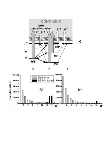
Figure 1: (a) Schematic illustration of BBR induced and field ionization processes occurred after excitation of the initial Na(16S) state, including redistribution of population over other $n^{\prime}L^{\prime}$ Rydberg states due to spontaneous and BBR induced transitions from the initial state. (b) Calculated spontaneous and BBR induced transition rates from the initial 16S state to other $n^{\prime}$P states. (c) Calculated spontaneous and BBR induced transition rates from the initial 16D state to other $n^{\prime}$P states.

The first contribution, $W_{BBR}$, is the direct BBR photoionization rate of the initially excited nL state, which will be discussed in Section II A. The second term, $W_{SFI}$, is the rate of the selective field ionization (SFI) of high $n^{\prime\prime}L^{\prime}$ Rydberg states, which are populated from the initial Rydberg state nL via absorption of BBR photons. This field ionization will be discussed in Section II C, while redistribution of population between Rydberg states will be described in Section II B. The third term, $W_{BBR}^{mix}$, is the total rate of BBR-induced photoionization of neighboring $n^{\prime}L^{\prime}$ Rydberg states, which are populated via spontaneous and BBR-induced transitions from the initial state. The last term, $W_{SFI}^{mix}$, is the rate of SFI of high-lying Rydberg $n^{\prime\prime}L^{\prime}$ states that are populated in a two-step process via absorption of BBR photons by atoms in $n^{\prime}L^{\prime}$ states (note, that here, in contrast to $W_{SFI}$, we consider lower $n^{\prime}L^{\prime}$, states which cannot be directly field ionized). These latter two ionization rates, which are related to population redistribution between Rydberg states, will be considered in Section II D . The atomic units are used below, unless specified otherwise.

II.1 Direct BBR photoionization.

Direct BBR-induced photoionization rate $W_{BBR}$ of a given nL state is calculated from the general formula SpencerIon :

$$W_{BBR}=c\int\limits_{\omega_{nL}}^{\infty}{\sigma_{\omega}\;\rho_{\omega}d\omega},$$ (3)

where c is the speed of light, $\omega_{nL}=1/\left({2n_{eff}^{2}}\right)$ is the photoionization threshold frequency for the nL Rydberg state with the effective principal quantum number $n_{eff}=\left({n-\delta_{L}}\right)$, where $\delta_{L}$ is a quantum defect, and $\sigma_{\omega}$ is the photoionization cross-section at the frequency $\omega$. The volume density $\rho_{\omega}$ of BBR photons at the temperature T is given by the Plank distribution:

$$\rho_{\omega}=\frac{{\omega^{2}}}{{\pi^{2}c^{3}\left[{\mathrm{e}^{\omega/\left({kT}\right)}-1}\right]}},$$ (4)

where kT is thermal energy in atomic units. For isotropic and non-polarized thermal radiation field, the value of $\sigma_{\omega}$ is determined by the radial matrix elements $R\left({nL\to E,L\pm 1}\right)$ of dipole transitions from discrete nL Rydberg states to the continuum states with L$\pm$1 and photoelectron energy E:

$$\sigma_{\omega}=\frac{{4\pi^{2}\omega}}{{3c\left({2L+1}\right)}}\sum\limits_{L^{\prime}=L\pm 1}{L_{max}R^{2}\left({nL\to E,L\pm 1}\right)},$$ (5)

where L_max is the largest of $L$ and $L^{\prime}$.

The main problem in the calculation of W_BBR for an arbitrary Rydberg state is thus to find the values of $R\left({nL\to E,L\pm 1}\right)$ and their frequency dependence. In order to achieve high accuracy of the matrix elements, numerical calculations should be used. In this work we used the semi-classical formulae derived by Dyachkov and Pankratov Dyachkov . In comparison with other semi-classical methods GDK ; Davydkin , this method is advantageous as it gives orthogonal and normalized continuum wavefunctions, which allow for the calculation of photoionization cross-sections with high accuracy. We have verified that photoionization cross-sections of the lower sodium S states calculated using the approach of Dyachkov are in good agreement with the sophisticated quantum-mechanical calculations by Aymar Aymar .

Approximate analytical expressions for W_BBR would also be useful, since they illustrate how the ionization rate depends on parameters n, L, and T. Such expressions can be obtained using the analytical formulae for bound-bound and bound-free matrix elements deduced by Goreslavsky, Delone and Krainov (GDK) GDK in the quasiclassical approximation. For the direct BBR-induced photoionization of an nL Rydberg state the cross-section is given by:

$$\sigma_{\omega}\left({nL\to E,L\pm 1}\right)=\qquad\qquad\qquad\qquad\qquad$$

$$=\frac{{4L^{4}}}{{9cn^{3}\omega}}\left[{K_{2/3}^{2}\left({\frac{{\omega L^{3}}}{{3}}}\right)+K_{1/3}^{2}\left({\frac{{\omega L^{3}}}{{3}}}\right)}\right],$$ (6)

where $K_{\nu}\left({x}\right)$ is the modified Bessel function of the second kind. This formula was initially derived to describe the photoionization of hydrogen atom. It was assumed that the formula can be extended to alkali atoms simply by replacing n by $n_{eff}=\left({n-\delta_{L}}\right)$, where $\delta_{L}$ is the quantum defect of the Rydberg state. In the reality, however, its accuracy in absolute values is acceptable only for truly hydrogen-like states with small quantum defects. A disadvantage of the GDK model is that it disregards non-hydrogenic phase factors in the overlap integrals of dipole matrix elements.

The main contribution to W_BBR in Eq. (3) is due to BBR frequencies near the ionization threshold frequency $\omega_{nL}$, because the bound-free dipole moments rapidly decrease with increasing $\omega$. For Rydberg states with n$\gg$1 and low L one has ($\omega$L³/3)$\ll$1. In this case Eq. (II.1) can be simplified to the form:

$$\sigma_{\omega}\left({nL\to E,L\pm 1}\right)\approx\qquad\qquad\qquad\qquad\qquad$$

$$\approx\frac{{1}}{{9cn^{3}}}\left[{\frac{{6^{4/3}\Gamma^{2}\left({2/3}\right)}}{{\omega^{7/3}}}+\frac{{6^{2/3}\Gamma^{2}\left({1/3}\right)}}{{\omega^{5/3}}}L^{2}}\right].$$ (7)

The combination of Eqs. (3), (4) and (II.1) yields:

$$W_{BBR}\approx\frac{{1}}{{\pi^{2}c^{3}n^{3}}}\int\limits_{\omega_{nL}}^{\infty}{\left[{2.22\,\omega^{-1/3}+2.63\,\omega^{1/3}L^{2}}\right]}\times$$

$$\times\frac{{d\omega}}{{\mathrm{e}^{\omega/\left({kT}\right)}-1}}.$$ (8)

The expression in square brackets is a slowly varying function of $\omega$. Taking into account that the main contribution to W_BBR is due to frequencies near the ionization threshold, one can replace $\omega$ by 1/(2n²). After such replacement the integral in Eq. (II.1) can be calculated analytically, and the final result is:

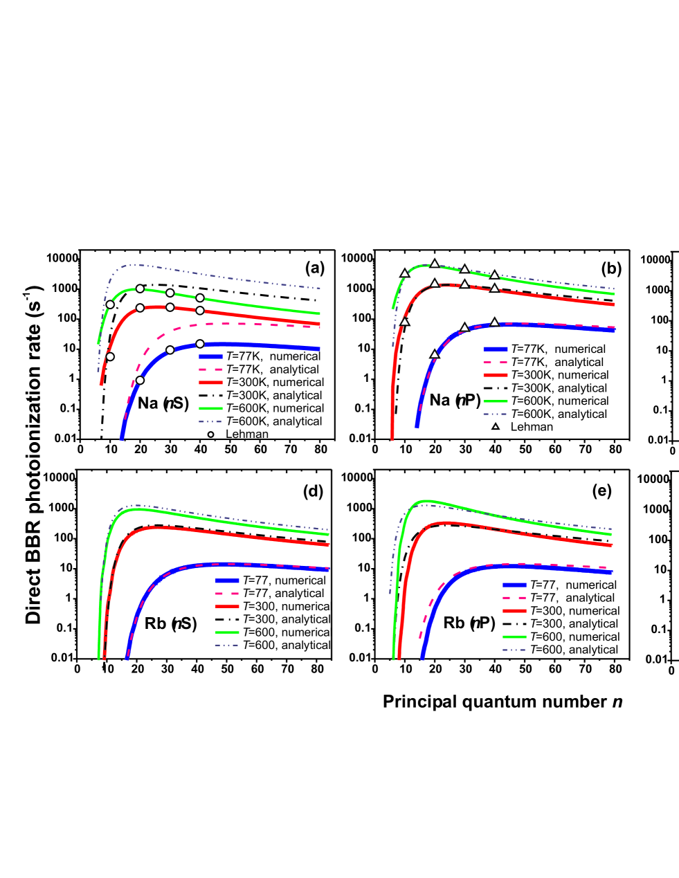
Figure 2: Direct BBR-induced photoionization rate of the sodium nS (a), nP (b), nD(c) and rubidium nS (d), nP (e) and nD (f) states with n=5-80 calculated at the ambient temperatures T=77, 300 and 600 K.

$$W_{BBR}\approx\frac{{kT}}{{\pi^{2}c^{3}}}\left[{\frac{{2.80}}{{n^{7/3}}}+\frac{{2.09L^{2}}}{{n^{11/3}}}}\right]\mathrm{ln}\left({\frac{{1}}{{1-\mathrm{exp}\left({-\frac{{\omega_{nL}}}{{kT}}}\right)}}}\right).$$ (9)

Equation (9) gives the approximate direct BBR photoionization rate in atomic units for T measured in Kelvins. Alternatively, it can be rewritten to yield W_BBR in the units of s^-1 for temperature T taken in Kelvins as follows:

$$W_{BBR}=C_{L}T\left[{\frac{{14423}}{{n^{7/3}}}+\frac{{10770L^{2}}}{{n^{11/3}}}}\right]\times\qquad\qquad\qquad$$

$$\times\mathrm{ln}\left({\frac{{1}}{{1-\mathrm{exp}\left({-\frac{{157890}}{{Tn^{2}}}}\right)}}}\right)\,\,\left[{\mathrm{s}^{-1}}\right].\quad$$ (10)

Here C_L is an L-dependent scaling coefficient, which will be discussed later. By replacing n with the effective principal quantum number, Eq. (II.1) can be used for quick estimations of direct BBR ionization rates for various Rydberg atoms and states. The precise values, however, should be calculated numerically.

The results of our numerical and analytical calculations of the direct BBR-induced photoionization rates for sodium and rubidium nS, nP and nD states with n=5-80 at the ambient temperatures T=77, 300 and 600 K are shown in Fig. 2. A good agreement of our numerical results obtained using the Dyachkov and Pankratov model with the theoretical data obtained by Lehman Lehman is observed. For the case of rubidium such comparison is not possible because no other published data are available, to the best of our knowledge.

It is also interesting and instructive to compare the results obtained by numeric calculation with those obtained using the analytical formula (II.1). Figure 2(a) shows a remarkable disagreement between the numerical and analytical results (assuming C_L=1) for sodium nS states, which are known to possess a large quantum defect ($\delta_{S}$=1.348). At the same time, Figs. 2(b) and 2(c) show that in the case of Na nP and nD states, which have smaller quantum defects ($\delta_{P}$=0.855 and $\delta_{D}$=0.015), the agreement between the numerical and analytical results is much better. This is not unexpected, since Eq. (II.1) is valid only for states with small quantum defects. Formally, the disagreement for the non-hydrogenic nS states stems from peculiarities of the asymptotic behavior of Bessel functions in Eq. (II.1) for states with $L\ll 1$: the analytical expression of GDK model yields close photoionization cross-section values for nS, nP and nD states, while the accurate numerical calculations yield significantly smaller cross-sections for sodium nS states [see Fig. 2(a)]. At the same time, one can see from Fig. 2(a) that shapes of the analytical curves are quite similar to the numerical ones. Therefore, one can simply introduce a scaling coefficient in Eq. (II.1) in order to make it valid also for nS states.

In order to illustrate that, in Figs. 2(d)-(f) we show the rescaled results of Eq. (II.1) for the case of Rb Rydberg atoms nS, nP, and nD states, which all have large quantum defects ($\delta_{L}$ = 3.13, 2.66, and 1.34, respectively). A good agreement between the analytical and numerical results was obtained when the rate obtained from Eq. (II.1) was scaled by a factor of C_S=0.2, C_P=0.2 and C_D=0.4 for the case of nS, nP, and nD states, respectively.

Our precise numerical data on W_BBR are summarized in Tables (1)-(6) of Appendix.

II.2 BBR-induced mixing of Rydberg states

BBR causes not only direct photoionization of the initially populated levels. It also induces transitions between neighboring Rydberg states, thus leading to a population redistribution Galvez1 ; Galvez2 ; PaperII . For example, after laser excitation of the Na 16S state, the BBR-induced transitions populate the neighboring $n^{\prime}$P states [Fig. 1(a)]. The calculations show that these states have significantly higher direct photoionization rates W_BBR than the 16S state itself. Hence, BBR-induced population transfer to $n^{\prime}$P state can noticeably affect the measured effective BBR ionization rate. The rates of spontaneous and BBR-induced transitions from the initial 16S and 16D states to a number of $n^{\prime}$P states have been calculated by us in PaperI and are shown in Figs. 1(b) and 1(c).

Importantly, absorption of BBR induces also transitions to higher Rydberg states, which are denoted as $n^{\prime\prime}$ in Fig. 1(a). These states can be field ionized by the electric field pulses usually applied in experiments in order to extract ions into channeltron or microchannel plate detectors.

II.3 Field ionization of high Rydberg states populated by BBR

Extraction electric field pulses, which are commonly used to extract ions from the ionization zone to the ionization detector, ionize Rydberg states with principal quantum numbers n exceeding some critical value $n_{c}$. This critical value $n_{c}$ depends on the amplitude of the applied electric field and it can be found from the approximate formula SFI

$$E_{c}\approx 3.2\cdot 10^{8}n_{c}^{-4}\quad\left(\mathrm{V/cm}\right).$$ (11)

were E_c is the critical electric field for $n_{c}$. Hence, if a BBR mediated process populates a state with $n^{\prime}\geq n_{c}$, this state will be ionized and thus will contribute to the detected ionization signal SpencerIon .

We calculated the radial matrix elements $R\left({nL\to n^{\prime}L^{\prime}}\right)$ of all dipole-allowed transitions to other $n^{\prime}L^{\prime}$ states with $L^{\prime}=(L\pm 1)$ using the semi-classical formulae of Dyachkov . The rate of a BBR-induced transition between the states $nL$ and $n^{\prime}L^{\prime}$ is expressed through the rate of spontaneous transitions given by the Einstein coefficient $A\left({nL\to n^{\prime}L^{\prime}}\right)$:

$$A\left({nL\to n^{\prime}L^{\prime}}\right)=\frac{{4}}{{3c^{3}}}\frac{{L_{max}}}{{2L+1}}R^{2}\left({nL\to n^{\prime}L^{\prime}}\right),$$

$$W\left({nL\to n^{\prime}L^{\prime}}\right)=A\left({nL\to n^{\prime}L^{\prime}}\right)\frac{{\omega_{nn^{\prime}}^{3}}}{{\mathrm{e}^{\omega_{nn^{\prime}}/\left({kT}\right)}-1}},$$ (12)

where $\omega_{nn^{\prime}}=1/(2n^{2})-1/(2n^{\prime 2})$ is the transition frequency. Note that spontaneous transitions are possible only to lower levels, while BBR leads to transitions both upwards and downwards.

The total rate $W_{SFI}$ of BBR transitions to all Rydberg states with $n^{\prime}\geq n_{c}$ was calculated by summing the individual contributions of $nL\to n^{\prime}L^{\prime}$ transitions given by Eq. (II.3):

$$W_{SFI}=\,\sum\limits_{n^{\prime}\geq n_{c}}{\,\sum\limits_{L^{\prime}=L\pm 1}{W\left({nL\to n^{\prime}L^{\prime}}\right)}}.$$ (13)

The values of $W_{SFI}$ were numerically calculated for various amplitudes E of the electric field pulses.

We also compared the numerical values with those obtained from the approximate analytical formulae, which has been derived with the bound-bound matrix elements of the GDK model:

$$W_{SFI}\approx\frac{{1}}{{\pi^{2}c^{3}n^{3}}}\times\qquad\qquad\qquad\qquad\qquad\qquad$$

$$\times\int\limits_{1/(2n^{2})-1/(2n_{c}^{2})}^{\quad\omega_{nL}}{\left[{2.22\,\omega^{-1/3}+2.63\,\omega^{1/3}L^{2}}\right]}\times$$

$$\times\frac{{d\omega}}{{\mathrm{e}^{\omega/\left({kT}\right)}-1}}.\qquad$$ (14)

The integration limits are chosen such that the integral accounts for transitions to those Rydberg states, for which $\left[1/(2n^{2})-1/(2n_{c}^{2})\right]<\omega<\omega_{nL}$ (i.e., states above the field ionization threshold). Integration of Eq. (II.3) gives another useful analytical formula that is similar to Eq. (II.1):

$$W_{SFI}=C_{L}T\left[{\frac{{14423}}{{n^{7/3}}}+\frac{{10770L^{2}}}{{n^{11/3}}}}\right]\times\qquad\qquad\qquad\qquad$$

$$\times\left(\mathrm{ln}\frac{{1}}{{1-\mathrm{exp}\left({\frac{{157890}}{{Tn_{c}^{2}}}-\frac{{157890}}{{Tn^{2}}}}\right)}}\,-\right.\qquad\qquad$$

$$-\left.\mathrm{ln}\frac{{1}}{{1-\mathrm{exp}\left({-\frac{{157890}}{{Tn^{2}}}}\right)}}\right)\left[\mathrm{s}^{-1}\right],\qquad$$ (15)

where T is in Kelvins.

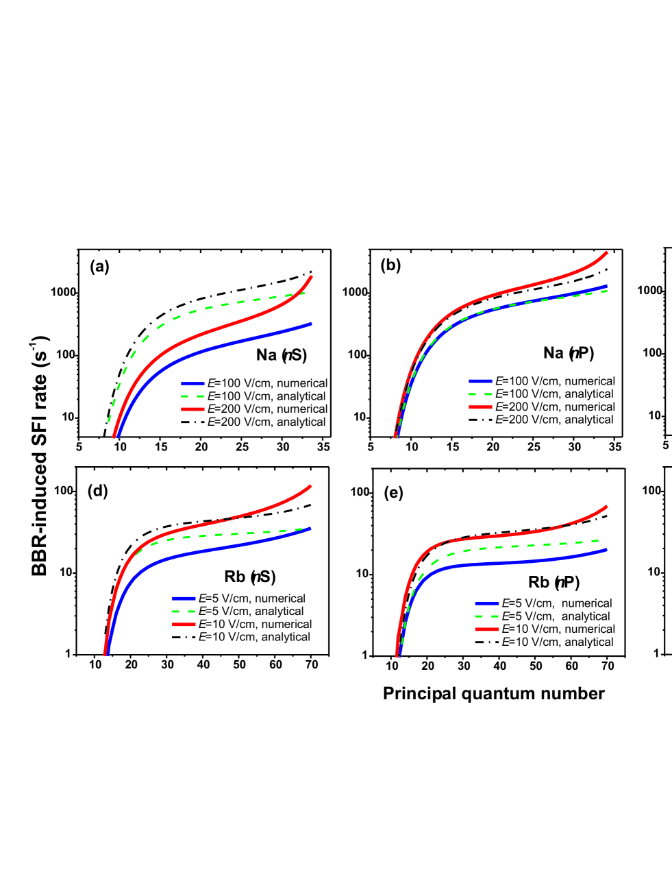
Figure 3: The calculated BBR-induced SFI rate W_SFI for (a) Na(nS), (b) Na(nP), and (c) Na(nD) states with n=5-35 at the electric field amplitudes of E=100 and 200 V/cm, and for the (d) Rb(nS), (e) Rb(nP), and (f) Rb(nD) states with n=5-80 at the electric field amplitudes of E=5 and 10 V/cm. In all cases the ambient temperature is T=300 K.

The obtained numerical and analytical data on W_SFI are presented in Fig. 3. For Na atoms, the calculations were made for the nS, nP and nD states with n=5-35 at the ambient temperature T=300 K [Figs. 3(a), 3(b) and 3(c)]. The amplitudes E of the extracting electric field pulse are chosen as 100 and 200 V/cm (corresponding to $n_{c}=42$ and 36, respectively). These values are close to those used in our recent atomic-beam experiment on ionization of Na atoms PaperI . Alternatively, Figs. 3(d), 3(e) and 3(f) show the calculated rates $W_{SFI}$ for nS, nP and nD states of Rb for the lower E values (5 V/cm and 10 V/cm corresponding to $n_{c}$=91 and $n_{c}$ =76, respectively), which are more adequate to experiments with Rydberg atoms in cold gases.

In order to achieve a better agreement between the analytical formula (II.3) and the results of numerical calculations, scaling coefficients $C_{L}$ in Eq. (II.3) were also introduced. The best agreement was obtained at $C_{S}=0.2$, $C_{P}=0.15$ and $C_{D}=0.3$ for the Rb nS, nP and nD states, respectively. In the case of nP and nD states of Na data such scaling was not necessary, while in the case of nS states of Na the best agreement [not shown in Fig. 3(a)] was found at $C_{S}=0.25$. The possibility to achieve a satisfactory agreement between the numerical and analytical data of Fig. 3 suggests that, using appropriate scaling coefficients, the analytical formula (II.3) is also suitable to quick estimates of BBR-induced SFI rates for various Rydberg atoms and states.

Our precise numerical data on $W_{SFI}$ are summarized in Tables (1)-(6) of Appendix.

II.4 Ionization of Rydberg states populated by BBR

In this section we shall analyze the influence of time evolution of populations of Rydberg states upon interaction with ambient BBR photons. The typical timing diagram of laser excitation of Rydberg states and detection of ions is shown in Fig. 4. Such scheme was used in our recent experiment on collisional ionization of Na Rydberg atoms PaperI . The first electric-field pulse is applied immediately after the laser excitation pulse in order to remove the atomic $A^{+}$ and molecular $A_{2}^{+}$ photoions produced by the laser pulse. Then atoms are allowed to interact with ambient BBR during the time interval (t₁, t₂). The second electric-field pulse extracts the ions, which have been produced by collisional and BBR-induced ionization, to the ion detector. The atomic and molecular ions were distinguished using a time-of-flight method. At the ground-state density of $5\times 10^{10}$cm^-3 the BBR ionization is the main source of atomic ions PaperI and the contribution from collisonal ionization of Penning type is negligible.

Let us consider first the simplest case of laser excitation of a single nS state. The evolution of the number $N_{A^{+}}$ of atomic ions produced via absorption of BBR photons by atoms in the initial nS state is given by

$$\frac{{dN_{A^{+}}\left({t}\right)}}{{dt}}=W_{BBR}N_{nS}\left({t}\right),$$ (16)

where $N_{nS}(t)=N_{nS}(t=0)\mathrm{exp}(-t/\tau_{eff}^{nS})$ is the total number of Rydberg atoms remaining in the nS state as a function of time, and $\tau_{eff}^{nS}$ is an effective lifetime of the $n$S state at a given ambient temperature. The registered photoions are produced during the time interval ($t_{1},t_{2}$). The total number of ions can then be found by integrating Eq. (16) from $t_{1}$ to $t_{2}$.

$$N_{A^{+}}=N_{nS}\left({t=0}\right)W_{BBR}\times\qquad\qquad\qquad$$

$$\times\tau_{eff}^{nS}\left[{\mathrm{exp}\left({-t_{1}/\tau_{eff}^{nS}}\right)-\mathrm{exp}\left({-t_{2}/\tau_{eff}^{nS}}\right)}\right],$$ (17)

This result can be rewritten by introducing an effective interaction time PaperI :

$$N_{A^{+}}=N_{nS}\left({t=0}\right)W_{BBR}t_{eff}^{nS},\qquad\qquad\qquad\qquad$$

$$t_{eff}^{nS}=\tau_{eff}^{nS}\left[{\mathrm{exp}\left({-t_{1}/\tau_{eff}^{nS}}\right)-\mathrm{exp}\left({-t_{2}/\tau_{eff}^{nS}}\right)}\right].$$ (18)

Blackbody radiation also induces transitions to other Rydberg states $n^{\prime}$P, as was discussed in Section II B. Evolution of populations of these states is described by the rate equation

$$\frac{{dN_{{n}^{\prime}P}\left({t}\right)}}{{dt}}=\left[W\left({nS\to{n}^{\prime}P}\right)+A\left({nS\to{n}^{\prime}P}\right)\right]\,N_{nS}\left({t}\right)-$$

$$-{N_{{n}^{\prime}P}\left({t}\right)}/{\tau_{eff}^{n^{\prime}P}},\qquad$$ (19)

where $A(n\mathrm{S}\to n^{\prime}\mathrm{P})$ and $W(n\mathrm{S}\to n^{\prime}\mathrm{P})$ are the rates of population of the $n^{\prime}$P state due to spontaneous transitions to lower levels and BBR induced transitions upwards and downwards from the initial nS state, and $\tau_{eff}^{nP}$ is the effective lifetime of the $n^{\prime}$P state.

Figure 4: Timing diagram of signals: (a) laser excitation pulse; (b) electric field pulses for the ion extraction; (c) atomic $A^{+}$ and molecular $A^{+}_{2}$ ion signals; (d) detector gates.

A combination of Eq. (II.4) with Eqs. (16) and (II.4) yields

$$W_{BBR}^{mix}\left({nS}\right)=\sum\limits_{{n}^{\prime}}{\frac{{\left[W\left({nS\to{n}^{\prime}P}\right)+A\left({nS\to{n}^{\prime}P}\right)\right]}}{\left(\tau_{eff}^{n^{\prime}P}\right)^{-1}-\left(\tau_{eff}^{nS}\right)^{-1}}}\times$$

$$\times W_{BBR}\left({{n}^{\prime}P}\right)\left({1-\frac{{t_{eff}^{nS}}}{{t_{eff}^{{n}^{\prime}P}}}}\right).\quad$$ (20)

The main contribution to the sum in Eq. (II.4) is from $n^{\prime}$P states with $n^{\prime}=n\pm 1$ [see Fig. 1(b)]. The effective BBR ionization rates for nP and nD states were determined in the same way as for nS states, taking into account the population transfer to both $n^{\prime}(L+1)$ and $n^{\prime}(L-1)$ states.

The rate $W_{SFI}^{mix}$ describes the second-order process of BBR-induced transitions from the neighboring $n^{\prime}L^{\prime}$ states to highly excited states $n^{\prime\prime}L^{\prime\prime}$ with $n^{\prime\prime}>n_{c}$ [see Fig. 5(a)], followed by ionization of these states by extracting electric field pulses. This rate can be calculated using the same Eq. (II.4), in which $W_{BBR}$ is replaced by $W_{SFI}$ and the summation is done over the states with $n^{\prime}<n_{c}$.

Our precise numerical data on $W_{BBR}^{mix}$ and $W_{SFI}^{mix}$ are summarized in Tables (1)-(6) of Appendix.

III Results of calculations and comparison with experiment

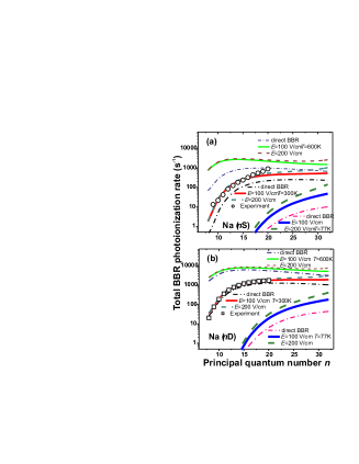
Figure 5: Calculated total BBR-induced ionization rates $W_{BBR}^{tot}$ for (a) nS and (b) nD states of Na with n=8-35 for the extracting electric field pulses of 100 V/cm and 200 V/cm at the ambient temperatures of T=77, 300 and 600 K. Experimental points are taken from Ref. PaperI .

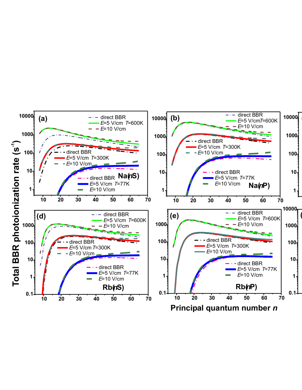
Figure 6: The calculated total BBR-induced ionization rates $W_{BBR}^{tot}$ for (a) Na(nS), (b) Na(nP), (c) Na(nD), (d) Rb(nS), (e) Rb(nP), and (d) Rb(nD) Rydberg states for the electric field amplitudes of 5 V/cm and 10 V/cm at the ambient temperatures of T=77 K, 300 K and 600 K.

Calculated total BBR-induced ionization rates $W_{BBR}^{tot}$ for Na nS, nP and nD states at the temperatures T = 77, 300, 600 K and for the extracting electric field pulses of E=100 V/cm and 200 V/cm, as well as their comparison with our experimental data from Ref. PaperI , are shown in Fig. 5. Since the values of $W_{BBR}^{tot}$ depend on the timing of the experiment (see Fig. 4), the calculations were performed for $t_{1}=0.3\,\mu$s and $t_{2}=2.1\,\mu$s, which were used in our experiment PaperI . At the 300 K temperature a good agreement is observed for nD states with n=8-20 and for nS states with n=8-15. At the same time, for nS states with $n>15$ the calculated ionization rates start to deviate from the experimental values; the measured values exceed the theoretical ones by a factor of 2.1 for n=20, and the shape of the experimental n-dependence differs from the theoretical one.

One possible explanation of such anomaly for nS states is related to their specific orbit that penetrates into the atomic core. The penetration causes a strong interaction between the Rydberg electron and the core, e.g., due to core polarization Aymar . This results in large quantum defect and a Cooper minimum in the photoionization cross-sections. This assumption is supported by the good agreement of theory and experiment for the hydrogen-like nD states, which have a small quantum defect and almost non-penetrating orbits.

Total BBR-induced ionization rates were also calculated for Na and Rb $n$S, $n$P and $n$D states in a broader range of $n$ and for lower amplitudes of the electric field pulses (5 V/cm and 10 V/cm). Such fields are more relevant to the experiments with cold Rydberg atoms, e.g., to ultracold plasma formation from cold Rydberg atoms clouds Robinson ; Li , since these experiments explore the atoms excited to relatively high Rydberg states that are ionized in weaker electric fields (35 V/cm for $n\sim 50$ and 10 V/cm for $n\sim 80$). The calculated ionization rates are presented in Fig. 6. It can be seen that SFI and BBR-induced level-mixing processes alter the shapes of n-dependences of total ionization rates $W_{BBR}^{tot}$, which effect is more pronounced at lower temperatures and larger n. As Fig. 6 has a logarithmic scale, the visible effect of additional processes looks small. However, from the tables of Appendix it can be seen that, e.g., for the Rb 65S state at $T$=300 K the total BBR ionization rate is twice larger than the direct photoionization rate (see Table 5).

Precise results of our numerical calculations for a five-step set of principal quantum numbers n are summarized in Tables (1)-(6) of Appendix. The values of ionization rates at the other n values can be obtained either by extrapolation or upon request from the authors of this paper.

IV Conclusion

We have calculated the total BBR-induced ionization rates of Na and Rb nS, nP and nD Rydberg states for principal quantum numbers n=8-65 at the ambient temperatures of 77, 300 and 600 K. Our calculations take into account the effect of BBR-induced mixing of Rydberg states and their field ionization by extracting electric field pulses. Useful analytical formulae have been derived, which allow for quick estimation of ionization rates and their dependences on the principal quantum number n. The numerical results are in a good agreement with our recent experiment data on Na nS and nD states, except for nS states with $n>15$, which is most probably associated with the Cooper minimum in the photoionization cross-section.

The obtained results show that BBR-induced redistribution of population over Rydberg states and their field ionization by extracting electric fields affect both the magnitudes of total ionization rates and shapes of their dependencies on the principal quantum number. This suggests that these processes are important and cannot be ignored in the calculations and measurements of BBR ionization rates. Equations (16)-(II.4), as well as the analytical formulae (9) and (II.3), can be used to calculate total ionization rates $W_{BBR}^{tot}$ under particular experimental conditions. The obtained numerical results may be helpful to the analysis of ionization signals measured in experiments on collisional ionization and spontaneous formation of ultracold plasma, since BBR-induced ionization is the main channel of delivering atomic ions. At the same time, as we have revealed that theoretical data for Na $n$S-states noticeably disagree with experiment at $15<n\leq 20$, new experimental data for Na and Rb in a broader range of principal quantum numbers would be of interest for the further improvement of theory, especially for the non-hydrogen-like states.

*

Table 1: Calculated BBR-induced ionization rates (s^-1) for Na at T=77 K

nS
$n$	$W_{BBR}$	$W_{SFI}$	$W_{SFI}$	$W_{BBR}^{mix}$	$W_{SFI}^{mix}$	$W_{SFI}^{mix}$	$W_{BBR}^{tot}$	$W_{BBR}^{tot}$
	direct	100V/cm	200V/cm		100V/cm	200V/cm	100V/cm	200V/cm
10	$1.56\times 10^{-7}$	$3.44\times 10^{-9}$	$7.71\times 10^{-9}$	$4.92\times 10^{-18}$	$3.55\times 10^{-9}$	$7.03\times 10^{-9}$	$2.12\times 10^{-7}$	$2.2\times 10^{-7}$
15	0.009	0.019	0.042	0.002	0.003	0.006	0.033	0.059
20	0.805	1.655	3.83	0.059	0.118	0.240	2.64	4.94
25	4.04	10.23	25.29	0.185	0.420	0.891	14.9	30.4
30	8.45	27.12	81.09	0.257	0.706	1.689	36.5	91.5
	$W_{BBR}$	$W_{SFI}$	$W_{SFI}$	$W_{BBR}^{mix}$	$W_{SFI}^{mix}$	$W_{SFI}^{mix}$	$W_{BBR}^{tot}$	$W_{BBR}^{tot}$
	direct	5V/cm	10V/cm		5V/cm	10V/cm	5V/cm	10V/cm
35	11.8	2.47	5.20	0.267	0.0488	0.107	14.6	17.4
45	14.6	4.12	9.09	0.195	0.0466	0.106	19.0	24.0
55	14.1	5.76	13.9	0.124	0.0412	0.102	20.1	28.3
65	12.6	8.01	23.6	0.0773	0.0377	0.111	20.7	36.4
nP
$n$	$W_{BBR}$	$W_{SFI}$	$W_{SFI}$	$W_{BBR}^{mix}$	$W_{SFI}^{mix}$	$W_{SFI}^{mix}$	$W_{BBR}^{tot}$	$W_{BBR}^{tot}$
	direct	100V/cm	200V/cm		100V/cm	200V/cm	100V/cm	200V/cm
10	$7.09\times 10^{-6}$	$3.49\times 10^{-7}$	$6.91\times 10^{-7}$	$4.75\times 10^{-8}$	$1.51\times 10^{-8}$	$2.99\times 10^{-8}$	$7.5\times 10^{-6}$	$7.85\times 10^{-6}$
15	0.0996	0.195	0.389	0.00111	0.00200	0.00409	0.298	0.493
20	5.22	10.2	20.5	0.0217	0.0455	0.0977	15.4	25.8
25	22.1	50.8	107	0.0545	0.132	0.308	73.1	130
30	42.4	120	290	0.0662	0.197	0.554	163	333
	$W_{BBR}$	$W_{SFI}$	$W_{SFI}$	$W_{BBR}^{mix}$	$W_{SFI}^{mix}$	$W_{SFI}^{mix}$	$W_{BBR}^{tot}$	$W_{BBR}^{tot}$
	direct	5V/cm	10V/cm		5V/cm	10V/cm	5V/cm	10V/cm
35	57.0	10.5	22.9	0.0726	0.0144	0.0318	67.6	80.0
45	66.2	16.2	37.1	0.0514	0.0135	0.0313	82.5	103
55	61.9	21.6	53.7	0.0320	0.0117	0.0297	83.5	116
65	53.8	28.6	86.5	0.0186	0.00997	0.0304	82.4	140
nD
$n$	$W_{BBR}$	$W_{SFI}$	$W_{SFI}$	$W_{BBR}^{mix}$	$W_{SFI}^{mix}$	$W_{SFI}^{mix}$	$W_{BBR}^{tot}$	$W_{BBR}^{tot}$
	direct	100V/cm	200V/cm		100V/cm	200V/cm	100V/cm	200V/cm
10	$1.11\times 10^{-4}$	$1.53\times 10^{-5}$	$2.98\times 10^{-5}$	$7.61\times 10^{-7}$	$4.96\times 10^{-7}$	$9.82\times 10^{-7}$	$1.28\times 10^{-4}$	$1.43\times 10^{-4}$
15	0.251	0.483	0.947	0.00270	0.00472	0.00953	0.742	1.21
20	6.59	12.7	25.2	0.0371	0.0762	0.158	19.4	32.0
25	22.6	50.0	104	0.0926	0.215	0.467	72.9	127
30	39.0	107	256	0.120	0.331	0.812	146	296
	$W_{BBR}$	$W_{SFI}$	$W_{SFI}$	$W_{BBR}^{mix}$	$W_{SFI}^{mix}$	$W_{SFI}^{mix}$	$W_{BBR}^{tot}$	$W_{BBR}^{tot}$
	direct	5V/cm	10V/cm		5V/cm	10V/cm	5V/cm	10V/cm
35	49.3	8.88	19.4	0.131	0.0239	0.0527	58.3	68.8
45	54.6	13.0	29.6	0.0995	0.0230	0.0528	67.7	84.3
55	49.8	16.7	41.5	0.0663	0.0204	0.0503	66.7	91.5
65	42.7	21.8	65.9	0.0424	0.0180	0.0519	64.6	109

Table 2: Calculated BBR-induced ionization rates (s^-1) for Na at T=300 K

nS
$n$	$W_{BBR}$	$W_{SFI}$	$W_{SFI}$	$W_{BBR}^{mix}$	$W_{SFI}^{mix}$	$W_{SFI}^{mix}$	$W_{BBR}^{tot}$	$W_{BBR}^{tot}$
	direct	100V/cm	200V/cm		100V/cm	200V/cm	100V/cm	200V/cm
10	7.50	1.33	2.34	13.6	3.02	4.88	25.5	28.3
15	114	39.4	70.2	78.6	24.2	39.6	256	302
20	223	99.2	185	77.6	29.2	49.2	429	534
25	254	155	314	53.6	26.2	46.9	489	669
30	242	218	537	34.2	23.2	46.9	518	861
	$W_{BBR}$	$W_{SFI}$	$W_{SFI}$	$W_{BBR}^{mix}$	$W_{SFI}^{mix}$	$W_{SFI}^{mix}$	$W_{BBR}^{tot}$	$W_{BBR}^{tot}$
	direct	5V/cm	10V/cm		5V/cm	10V/cm	5V/cm	10V/cm
35	217	19.3	39.5	22.6	1.55	3.29	261	283
45	166	22.8	49.1	10.2	1.04	2.30	200	227
55	126	27.3	64.2	5.15	0.780	1.87	159	197
65	97.4	35.0	100	2.80	0.652	1.86	136	202
nP
$n$	$W_{BBR}$	$W_{SFI}$	$W_{SFI}$	$W_{BBR}^{mix}$	$W_{SFI}^{mix}$	$W_{SFI}^{mix}$	$W_{BBR}^{tot}$	$W_{BBR}^{tot}$
	direct	100V/cm	200V/cm		100V/cm	200V/cm	100V/cm	200V/cm
10	79.92	15.99	25.84	2.426	0.8949	1.456	99.23	109.6
15	778.2	240.9	393.6	17.82	5.476	9.174	1042	1199
20	1295	501.8	845.4	19.05	6.384	11.24	1823	2171
25	1374	709.0	1272	13.50	5.610	10.76	2102	2670
30	1253	932.0	1919	8.444	4.660	10.56	2198	3191
	$W_{BBR}$	$W_{SFI}$	$W_{SFI}$	$W_{BBR}^{mix}$	$W_{SFI}^{mix}$	$W_{SFI}^{mix}$	$W_{BBR}^{tot}$	$W_{BBR}^{tot}$
	direct	5V/cm	10V/cm		5V/cm	10V/cm	5V/cm	10V/cm
35	1090	79.97	169.6	6.145	0.3428	0.7388	1177	1267
45	795.2	89.28	198.3	2.830	0.2290	0.5203	887.5	996.9
55	586.0	102.1	247.0	1.419	0.1679	0.4172	689.7	834.8
65	441.8	124.9	366.0	0.7254	0.1267	0.3768	567.5	808.9
nD
$n$	$W_{BBR}$	$W_{SFI}$	$W_{SFI}$	$W_{BBR}^{mix}$	$W_{SFI}^{mix}$	$W_{SFI}^{mix}$	$W_{BBR}^{tot}$	$W_{BBR}^{tot}$
	direct	100V/cm	200V/cm		100V/cm	200V/cm	100V/cm	200V/cm
10	157.5	37.01	59.22	13.71	2.596	4.237	210.8	234.7
15	890.1	268.2	434.4	39.52	8.003	13.30	1206	1377
20	1253	467.7	782.0	36.76	8.176	14.05	1765	2086
25	1244	613.5	1094	26.17	6.907	12.61	1891	2377
30	1099	774.0	1592	17.38	5.679	11.70	1896	2720
	$W_{BBR}$	$W_{SFI}$	$W_{SFI}$	$W_{BBR}^{mix}$	$W_{SFI}^{mix}$	$W_{SFI}^{mix}$	$W_{BBR}^{tot}$	$W_{BBR}^{tot}$
	direct	5V/cm	10V/cm		5V/cm	10V/cm	5V/cm	10V/cm
35	936.2	65.00	137.7	12.31	0.4207	0.8980	1014	1087
45	666.5	70.18	155.6	6.040	0.2783	0.6197	743.0	828.8
55	483.1	78.52	189.6	3.240	0.2025	0.4856	565.1	676.4
65	360.0	94.60	277.3	1.849	0.1557	0.4332	456.6	639.6

Table 3: Calculated BBR-induced ionization rates (s^-1) for Na at T=600 K

nS
$n$	$W_{BBR}$	$W_{SFI}$	$W_{SFI}$	$W_{BBR}^{mix}$	$W_{SFI}^{mix}$	$W_{SFI}^{mix}$	$W_{BBR}^{tot}$	$W_{BBR}^{tot}$
	direct	100V/cm	200V/cm		100V/cm	200V/cm	100V/cm	200V/cm
10	284.4	41.90	71.08	1396	187.6	294.9	1910	2046
15	910.1	185.6	321.5	1396	237.4	378.9	2729	3007
20	991.5	290.5	526.8	770.7	175.8	289.9	2229	2579
25	874.7	378.8	748.8	411.1	130.9	229.0	1796	2264
30	728.5	489.6	1172	229.0	105.5	208.4	1553	2338
	$W_{BBR}$	$W_{SFI}$	$W_{SFI}$	$W_{BBR}^{mix}$	$W_{SFI}^{mix}$	$W_{SFI}^{mix}$	$W_{BBR}^{tot}$	$W_{BBR}^{tot}$
	direct	5V/cm	10V/cm		5V/cm	10V/cm	5V/cm	10V/cm
35	601	42.9	87.6	139	7.04	14.8	790	843
45	416	48.3	104	57.1	4.46	9.82	526	586
55	299	56.5	132	27.5	3.25	7.76	386	467
65	222	71.3	203	14.6	2.67	7.57	311	448
nP
$n$	$W_{BBR}$	$W_{SFI}$	$W_{SFI}$	$W_{BBR}^{mix}$	$W_{SFI}^{mix}$	$W_{SFI}^{mix}$	$W_{BBR}^{tot}$	$W_{BBR}^{tot}$
	direct	100V/cm	200V/cm		100V/cm	200V/cm	100V/cm	200V/cm
10	2580	353.0	554.1	190.1	31.47	49.95	3155	3374
15	6054	1054	1681	279.2	45.01	73.60	7433	8088
20	5900	1433	2364	173.8	34.97	60.14	7541	8497
25	4884	1715	3015	96.59	26.01	48.63	6722	8044
30	3898	2077	4183	52.98	19.78	43.40	6048	8178
	$W_{BBR}$	$W_{SFI}$	$W_{SFI}$	$W_{BBR}^{mix}$	$W_{SFI}^{mix}$	$W_{SFI}^{mix}$	$W_{BBR}^{tot}$	$W_{BBR}^{tot}$
	direct	5V/cm	10V/cm		5V/cm	10V/cm	5V/cm	10V/cm
35	3115	177.6	375.1	35.25	1.458	3.135	3330	3529
45	2049	188.9	417.8	14.72	0.9238	2.094	2254	2484
55	1426	210.8	508.0	7.008	0.6582	1.632	1644	1942
65	1029	254.5	742.4	3.470	0.4856	1.439	1288	1777
35	3115	177.6	375.1	35.25	1.458	3.135	3330	3529
nD
$n$	$W_{BBR}$	$W_{SFI}$	$W_{SFI}$	$W_{BBR}^{mix}$	$W_{SFI}^{mix}$	$W_{SFI}^{mix}$	$W_{BBR}^{tot}$	$W_{BBR}^{tot}$
	direct	100V/cm	200V/cm		100V/cm	200V/cm	100V/cm	200V/cm
10	3679	506.3	787.9	750.7	68.35	108.5	5004	5326
15	6226	1052	1666	631.2	58.47	94.75	7968	8618
20	5547	1286	2106	368.8	40.12	67.39	7242	8090
25	4405	1458	2549	211.4	28.43	50.80	6103	7216
30	3434	1709	3438	124.9	21.11	42.54	5288	7039
	$W_{BBR}$	$W_{SFI}$	$W_{SFI}$	$W_{BBR}^{mix}$	$W_{SFI}^{mix}$	$W_{SFI}^{mix}$	$W_{BBR}^{tot}$	$W_{BBR}^{tot}$
	direct	5V/cm	10V/cm		5V/cm	10V/cm	5V/cm	10V/cm
35	2702	143.5	302.9	81.66	1.594	3.390	2929	3090
45	1733	148.1	327.0	36.94	0.9921	2.202	1919	2099
55	1185	162.0	389.4	19.08	0.6971	1.667	1367	1595
65	844.1	192.7	562.0	10.72	0.5188	1.438	1048	1418

Table 4: Calculated BBR-induced ionization rates (s^-1) for Rb at T=77 K

nS
$n$	$W_{BBR}$	$W_{SFI}$	$W_{SFI}$	$W_{BBR}^{mix}$	$W_{SFI}^{mix}$	$W_{SFI}^{mix}$	$W_{BBR}^{tot}$	$W_{BBR}^{tot}$
	direct	5V/cm	10V/cm		5V/cm	10V/cm	5V/cm	10V/cm
10	$3.34\times 10^{-12}$	$4.54\times 10^{-13}$	$9.46\times 10^{-13}$	$3.36\times 10^{-13}$	$4.36\times 10^{-14}$	$9.21\times 10^{-14}$	$4.18\times 10^{-12}$	$4.72\times 10^{-12}$
20	0.2826	0.04174	0.08730	0.005807	$7.58\times 10^{-4}$	0.001622	0.3309	0.3773
30	6.541	1.108	2.343	0.04932	0.006986	0.01519	7.706	8.949
40	12.61	2.740	5.967	0.04750	0.008213	0.01840	15.41	18.64
50	13.91	4.201	9.678	0.03120	0.007135	0.01687	18.15	23.64
60	12.97	5.813	14.96	0.01917	0.006156	0.01615	18.81	27.97
65	12.21	6.863	19.53	0.01502	0.005856	0.01688	19.10	31.78
nP
10	$2.96\times 10^{-10}$	$3.84\times 10^{-11}$	$8.1\times 10^{-11}$	$2.51\times 10^{-13}$	$3.39\times 10^{-14}$	$7.1\times 10^{-14}$	$3.35\times 10^{-10}$	$3.77\times 10^{-10}$
20	0.489	0.0636	0.136	0.00443	$6.31\times 10^{-4}$	0.00132	0.558	0.631
30	7.21	1.02	2.22	0.0412	0.00656	0.0139	8.28	9.49
40	11.8	2.08	4.65	0.0447	0.00887	0.0193	14.0	16.5
50	11.9	2.83	6.70	0.0321	0.00854	0.0195	14.8	18.7
60	10.5	3.60	9.49	0.0212	0.00797	0.0201	14.1	20.0
65	9.65	4.09	11.9	0.0171	0.00785	0.0217	13.8	21.6
nD
10	$5.11\times 10^{-7}$	$6.76\times 10^{-8}$	$1.42\times 10^{-7}$	$4.23\times 10^{-9}$	$5.57\times 10^{-10}$	$1.18\times 10^{-9}$	$5.83\times 10^{-7}$	$6.58\times 10^{-7}$
20	1.66	0.227	0.475	0.0149	0.00207	0.00442	1.90	2.15
30	15.7	2.46	5.19	0.0710	0.0110	0.0237	18.2	21.0
40	24.7	4.99	10.8	0.0662	0.0127	0.0280	29.7	35.6
50	25.4	7.15	16.5	0.0450	0.0113	0.0264	32.6	41.9
60	22.9	9.60	24.9	0.0287	0.0101	0.0260	32.5	47.8
65	21.3	11.3	32.5	0.0229	0.00969	0.0277	32.6	53.9

Table 5: Calculated BBR-induced ionization rates (s^-1) for Rb at T=300 K

nS
$n$	$W_{BBR}$	$W_{SFI}$	$W_{SFI}$	$W_{BBR}^{mix}$	$W_{SFI}^{mix}$	$W_{SFI}^{mix}$	$W_{BBR}^{tot}$	$W_{BBR}^{tot}$
	direct	5V/cm	10V/cm		5V/cm	10V/cm	5V/cm	10V/cm
10	0.604	0.0195	0.0390	0.408	0.0113	0.0228	1.04	1.07
20	183	7.58	15.3	20.8	0.633	1.30	212	220
30	235	14.8	30.3	9.25	0.390	0.819	260	276
40	189	18.5	39.2	3.70	0.227	0.492	211	232
50	143	21.9	49.1	1.67	0.150	0.344	167	194
60	109	26.7	67.0	0.842	0.113	0.288	137	177
65	96.1	30.3	83.9	0.619	0.103	0.287	127	181
nP
10	3.69	0.102	0.206	0.0598	0.00432	0.00873	3.85	3.96
20	300	9.25	19.0	8.14	0.311	0.626	317	327
30	294	13.0	27.3	4.87	0.255	0.520	312	327
40	207	13.8	30.0	2.20	0.173	0.363	223	240
50	144	14.7	33.8	1.07	0.126	0.278	160	179
60	103	16.5	42.3	0.568	0.103	0.246	120	146
65	87.8	18.0	51.0	0.426	0.0965	0.251	106	140
nD
10	27.8	0.782	1.58	2.73	0.0532	0.108	31.4	32.2
20	540	18.7	37.6	21.4	0.626	1.28	581	600
30	517	27.3	55.9	10.4	0.439	0.908	555	584
40	381	31.6	66.9	4.60	0.282	0.600	418	453
50	277	36.2	81.2	2.25	0.199	0.444	315	360
60	205	43.5	110	1.20	0.157	0.385	250	316
65	179	49.1	138	0.904	0.146	0.391	229	318

Table 6: Calculated BBR-induced ionization rates (s^-1) for Rb at T=600 K

nS
$n$	$W_{BBR}$	$W_{SFI}$	$W_{SFI}$	$W_{BBR}^{mix}$	$W_{SFI}^{mix}$	$W_{SFI}^{mix}$	$W_{BBR}^{tot}$	$W_{BBR}^{tot}$
	direct	5V/cm	10V/cm		5V/cm	10V/cm	5V/cm	10V/cm
10	81.20	1.429	2.838	177.4	2.395	4.806	262.4	266.2
20	941.6	26.22	52.51	259.5	4.569	9.340	1232	1263
30	734.1	35.55	72.58	68.99	1.925	4.022	840.6	879.7
40	500.8	40.35	85.19	23.30	1.009	2.181	565.4	611.4
50	350.5	45.92	102.7	9.740	0.6394	1.458	406.8	464.4
60	255.3	54.93	137.1	4.738	0.4709	1.188	315.4	398.3
65	220.8	61.92	170.6	3.445	0.4253	1.176	286.6	396.0
nP
10	373.9	5.011	10.06	20.19	0.6466	1.299	399.7	405.5
20	1690	30.95	63.33	100.7	2.073	4.156	1824	1858
30	1009	30.95	64.80	35.35	1.170	2.375	1077	1112
40	592.4	30.00	64.98	13.44	0.7148	1.488	636.5	672.3
50	374.1	30.71	70.43	6.029	0.4986	1.086	411.3	451.6
60	252.3	33.85	86.50	3.076	0.3940	0.9362	289.6	342.8
65	211.3	36.78	103.7	2.279	0.3675	0.9453	250.7	318.2
nD
10	1263	17.45	34.98	279.7	2.919	5.900	1563	1584
20	2696	57.56	115.5	220.0	3.948	8.007	2978	3040
30	1681	63.97	130.5	71.48	2.059	4.235	1819	1887
40	1051	68.29	144.0	27.59	1.211	2.556	1148	1225
50	699.6	75.56	168.9	12.59	0.8201	1.814	788.6	883.0
60	492.7	89.13	223.8	6.510	0.6320	1.534	589.0	724.5
65	420.5	100.1	280.1	4.847	0.5827	1.544	526.1	706.9

References

- (1) T. F. Gallagher and W. E. Cooke, Phys. Rev. Lett. 42, 835-839 (1979).
- (2) W. P. Spencer, A. G. Vaidyanathan, D. Kleppner, and T. W. Ducas, Phys. Rev. A 26, 1490-1493 (1982).
- (3) G. F. Hildebrandt, E. J. Beiting, C. Higgs, G. J. Hatton, K. A. Smith, F. B. Dunning, and R. F. Stebbings, Phys. Rev. A 23, 2978-2982 (1981).
- (4) W. P. Spencer, A. G. Vaidyanathan, D. Kleppner, and T. W. Ducas, Phys. Rev. A 25, 380-384 (1982).
- (5) T. F. Gallagher, Rydberg Atoms (Cambridge: Cambridge University Press) (1994).
- (6) J. W. Farley and W. H. Wing, Phys. Rev. A 23, 2397-2424 (1981).
- (7) E. J. Galvez, J. R. Lewis, B. Chaudhuri, J. J. Rasweiler, H. Latvakoski, F. De Zela, E. Massoni, and H. Castillo, Phys. Rev. A 51, 4010-4017 (1995).
- (8) E. J. Galvez, C. W. MacGregor, B. Chaudhuri, S. Gupta, E. Massoni and F. De Zela, Phys. Rev. A 55, 3002-3006 (1997).
- (9) M. P. Robinson, B. Laburthe Tolra, Michael W. Noel, T. F. Gallagher and P. Pillet, Phys. Rev. Let. 85, 4466 (2000).
- (10) W. Li, M. W. Noel, M. P. Robinson, P. J. Tanner, T. F. Gallagher, D. Comparat, B. Laburthe Tolra, N. Vanhaecke, T. Vogt, N. Zahzam, P. Pillet, D. A. Tate, Phys. Rev. A 70, 042713 (2004).
- (11) I. I. Ryabtsev, D. B. Tretyakov, I. I. Beterov, N. N. Bezuglov, K. Miculis and A. Ekers, J. Phys. B 38, S17 (2005).
- (12) G. W. Lehman, J. Phys. B: At. Mol. Phys. 16 2145-2156 (1983).
- (13) L. G. Dyachkov and P. M. Pankratov, J. Phys. B 27, 461 (1994).
- (14) S. P. Goreslavsky, N. B. Delone and V. P. Krainov, Sov. Phys. JETP, 55 246 (1982)
- (15) V. A. Davydkin and B. A. Zon, Opt. Spectr. 51 13 (1981).
- (16) M. Aymar, J. Phys. B 11, 1413 (1978).
- (17) R. F. Stebbings, C. J. Latimer, W. P. West, F. B. Dunning, and T. B. Cook, Phys. Rev. A 12, 1453 (1975); T. Ducas, M. G. Littman, R. R. Freeman, and D. Kleppner, Phys. Rev. Lett. 35, 366 (1975); T. F. Gallagher, L. M. Humphrey, R. M. Hill, and S. A. Edelstein, Phys. Rev. Lett. 37, 1465 (1976).
- (18) K. Miculis, I. I. Beterov, N. N. Bezuglov, I. I. Ryabtsev, D. B. Tretyakov, A. Ekers and A. N. Klucharev, Phys.B: At. Mol. Opt. Phys. 38 1811 (2005).
- (19) I. I. Beterov, D. B. Tretyakov, I. I. Ryabtsev, N. N. Bezuglov, K. Miculis, A. Ekers and A. N. Klucharev, J. Phys. B: At. Mol. Opt. Phys. 38 4349 (2005).