The Micromegas detector of the CAST experiment

Abstract

A low background Micromegas detector has been operating in the CAST experiment at CERN for the search of solar axions during the first phase of the experiment (2002-2004). The detector, made out of low radioactivity materials, operated efficiently and achieved a very low level of background rejection ($5\times 10^{-5}$ counts keV^-1cm^-2s^-1) without shielding.

1 Introduction

The CAST experiment [andriamonje:07b, zioutas:05a] uses three different types of detectors to detect the X-rays originated from the conversion of the axions inside a magnet: a time projection chamber autiero:06aTPC,, an X-ray telescope [kuster:06a], and a Micromegas detector. The Micromegas detector of CAST is a gaseous detector optimized for the detection of low energy ($1$–$10\,\rm{keV}$) X-ray photons. It is based on the micropattern detector technology of MICROMEGAS (MICROMEsh GAseous Structure) developed in the mid 90’s [giomataris:96a, giomataris:98a, charpak:02a]. collar:00a first suggested the advantages of using the Micromegas for such low-threshold, low-background measurements as required by the CAST experiment. These advantages include sensitivity at the keV and sub keV energy region where very good energy resolution can be achieved, excellent spatial resolution, one dimensional or X-Y readout capability, stability, construction simplicity and low cost. In addition, the proper choice of construction materials would lead to a detector appropriate for low background measurements.

The CAST Micromegas group designed and constructed a low background detector, the very first made with an X-Y readout structure, optimized for the efficient detection of the $1$–$10\,\rm{keV}$ photons. Several detectors have been developed during the course of the CAST running, each new one with increasingly improved characteristics replacing the older module during shutdown and maintenance periods. The detector is mounted on one of the two west superconducting magnet apertures looking for ’sunrise’ axions converted into X-ray photons that will enter the detector active volume perpendicularly to the X-Y strip plane.

2 Detector description

The principle of operation of the Micromegas detector designed for the CAST experiment is sketched in figure 1. A photon, after traversing a vacuum buffer space, enters the conversion-drift region, filled with a mixture of Argon-Isobutane ($95\%$–$5\%$), where it generates a photoelectron via the photoelectric effect. The photoelectron travels a short distance during which it creates ionization electrons. The electrons drift in a field of about 250 V$/$cm, until they reach and funnel through the micromesh and into the amplification region where a strong field of about $40\,\rm{kV}\,\rm{cm}^{-1}$ causes an avalanche. The resulting electron cluster is collected on the X-Y strips of the anode plane. The maximum achievable gain is about $10^{5}$, but for CAST gains of $5\times 10^{3}$ up to $10^{4}$ are sufficient to achieve the required threshold (around $1\,\rm{keV}$).

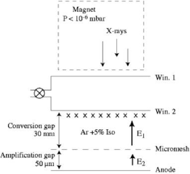
Figure 1: The Micromegas CAST detector.

The main sources of background are cosmic rays and natural radioactivity. Special care has been taken in the materials used for the construction of this Micromegas detector in order to reduce the natural radioactivity. Other developments have been necessary in order to optimize this detector given the aim and the environment of the experiment. A description of the most important elements specific to the CAST Micromegas detector are given below.

2.1 Mechanical structure

The detector frame consists of Plexiglas cylinders held together via plastic bolts. The drift and multiplication electrodes are attached on these cylinders. Figure 2 shows the mechanical structure of the detector. The conversion region can be $2.5$ or $3\,\rm{cm}$ thick and is formed between a $4\,\mu\rm{m}$ thick aluminized polypropylene window, glued on stainless steel or aluminum strongback, capable of holding vacuum at the magnet side, and the micromesh plane. The window of the conversion region also serves as the cathode for the drift field. The amplification region is only $50(100)\,\mu\rm{m}$ thick and is formed between the micromesh plane and the charge collection plane with the help of pillars spaced $1\,\rm{mm}$ apart. The micromesh is made of $4\,\mu\rm{m}$ thick Copper and is fabricated at CERN [delbart:02a].

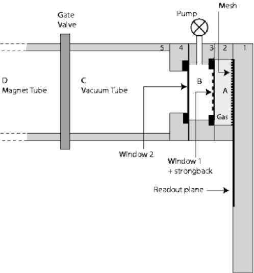
Figure 2: The mechanical design of the detector. The drift electrode is attached on disk 3. The micromesh holds on disk 2 and disk 4 is used to hold an extra vacuum window. The drawing is not made to scale.

2.2 Differential pumping

The detector is fastened to one of the magnet bores with the help of an aluminum tube and a flange. A gate valve separates the magnet volume from the tube volume. In order to couple a gaseous detector with a vacuum environment, keeping the maximum transparency to X-ray photons and a minimum vacuum leak, the solution of two windows with a differential pumping was adopted. The two windows are made out of a thin film of $4\,\mu\rm{m}$ polypropylene. The first window, that undergoes a pressure difference of $1\,\rm{bar}$, is glued on a strongback with a 94.6% transparency. The two windows delimit 3 zones that can be seen in figure 2. Zone A is the gaseous detector at a pressure of $1\,\rm{bar}$. Zone B is the vacuum gap at a pressure of $5\times 10^{-4}\,\rm{mbar}$ obtained with the pumping group. Zone C is the vacuum tube at a pressure of $5\times 10^{-7}\,\rm{mbar}$ in the magnet. The leak of the first window is proportional to the differential pressure between zone A and B, i.e., $1\,\rm{bar}$. This differential pressure imposes the use of a strongback. The leak for this window due to its porosity, tested with zone A full of helium, is $4\times 10^{-5}\,\rm{mbar}\,\rm{l}\,\rm{s}^{-1}$. As the differential pressure between zones B and C is only $5\times$10${}^{-4}\,\rm{bar}$, a strongback is not needed. The net leak for this window when zone A is full of helium, has been measured to be $3\times 10^{-9}\,\rm{mbar}\,\rm{l}\,\rm{s}^{-1}$. The leak on the first window has been evacuated by the pump. The pump system used for this application is made of a small dry turbo pump (magnetic bearing) and of a dry primary pump. The convolution of the transmission of the two windows together with the conversion efficiency of photons in the detector gas (Argon with 5% Isobutane) over the energy spectrum of solar axions between $2$ and $10\,\rm{keV}$ results in an combined efficiency of 85%. For sub-kev sensitivity a more efficient gas, like Xenon, could be used as well as thinner polypropylene windows.

2.3 Charge collection in two dimensions

The charge collection strips comprise an X-Y structure out of electrically connected pads see figure 3. The connections for the formation of the X-strips are on the one side of the doubly copper clad Kapton, while the connections for the Y-strips are made at the other side, with the help of metalized holes on the Y-pads. Each CAST detector has 192 X and 192 Y strips of $350\,\mu\rm{m}$ pitch. The active area therefore is about $45\,\rm{cm}^{2}$. The Kapton with the X and Y strips and the readout lines is glued on a paddle shaped plexiglass piece of the Micromegas structure, where the readout connectors are also fastened. New improvements are underway combining an integrated Micromegas and a CMOS micro-pixel anode plane [colas:04a, giomataris:06a].

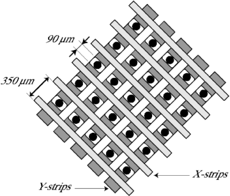
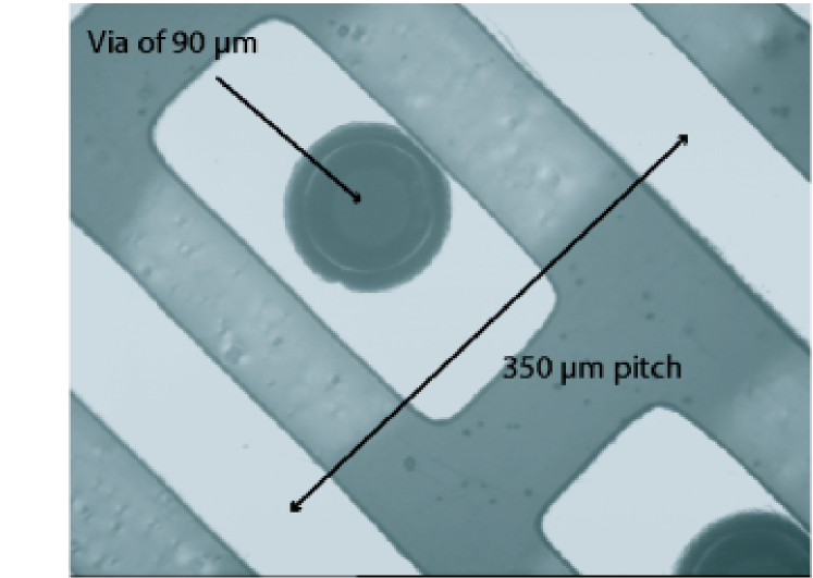
Figure 3: The X-Y strip charge collection structure. The strip pitch is $350\,\mu\rm{m}$. The X srips are those in light grey and the Y-strips, in the underneath layer, in dark grey. The metalized holes of 90 $\mu$m, allow the surface charge collection for the Y-strips.

2.4 Readout electronics and data acquisition

The charge on the X or Y strips is read out with the help of four Front End (FE) electronic cards based on the Gassplex chip [Santiard:94a] controlled by a CAEN sequencer (V 551B) with two CRAM (V550) modules in a VME crate [Geralis:03a].

One FE card integrates 96 signals (96 strips) and operates at a maximum clock speed of 1 MHz. It provides a multilevel output where each level corresponds to the result of the integration of the signal from a particular strip. The cards are powered by a 6V power supply (positive and negative). The Sequencer provides the proper timing signals (Clock, Track and Hold and Reset) to the FE cards. The CRAM modules integrate and store the total charge of each channel indicated by the signal provided by the FE cards until the software reads the data and transfers them to the PC for permanent storage and analysis. The signal for triggering the Micromegas device is obtained through the micromesh signal. The output of the preamplifier is subsequently shaped and amplified to produce the appropriate trigger signal. Because of the low rates involved (1 Hz) the zero suppression and pedestal subtraction capabilities of the CAEN modules are not used and all strip data are recorded.

The features of this Micromegas detector also include the recording of the mesh pulse via a high rate sampling VME Digitizing Board, the MATACQ Board [breton:05a]. This board, based on the MATACQ IC, can code 4 analog channels of bandwidth up to 300 MHz over 12 bits dynamic range and a sampling frequency reaching up to 2 GHz and over 2520 usable points. One of these channels is used to record the time structure of the mesh pulse. Signal events have a characteristic mesh pulse that will be used in order to reject events with unexpected shapes as background events. figure 4 shows a schematic of the Micromegas trigger and readout.

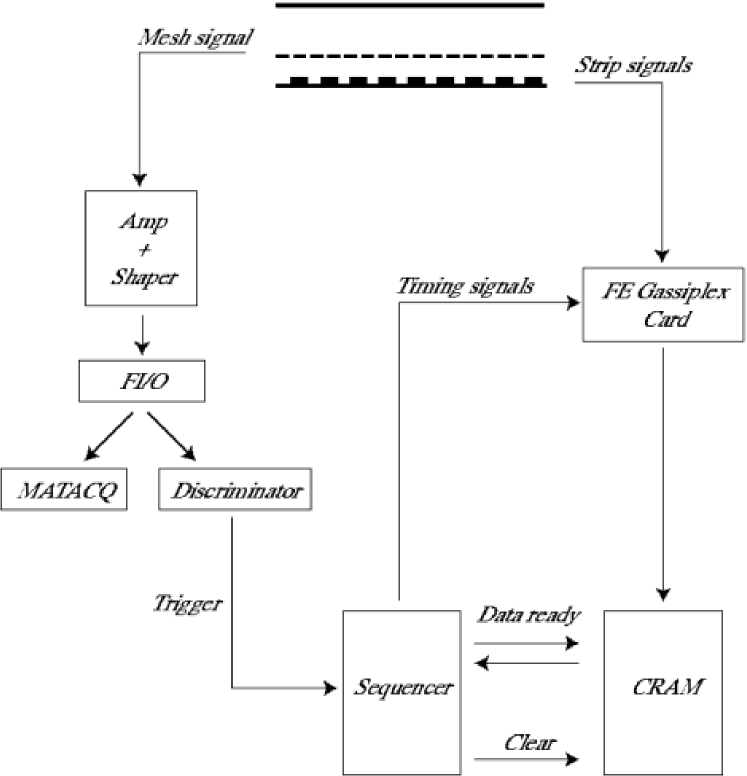
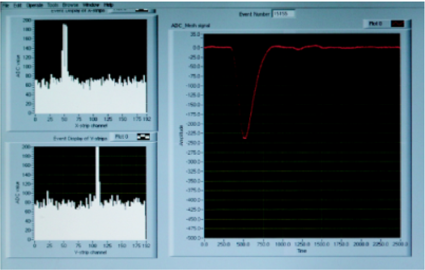
Figure 4: Left: Trigger and readout logic. Right: Event display showing the distribution of X and Y strip charges and the MATACQ pulse.

The data acquisition and monitoring system is based on the LabView software package, of National Instruments, running on a PC with either the Linux RedHat 7.3.1 (CERN release) or the Windows 2000 operating system. A dual boot PC is used to connect to the VME Controller and run the data acquisition software. The connection is performed via a PCI-MXI2 card sitting on the PCI bus of the PC, a VME-MXI2 controller card sitting on the VME and a 20 m long MXI2 cable connecting these two cards. The DAQ system runs on Linux since it provides the facilities of the CASTOR automatic data archiving system and the xntp software for the synchronization of the PC clock to the GPS universal time. The online software is controlled by LabView virtual modules that initialize the run (allowing parameters to be changed) and monitor its status. An event display is used to view the strip charges and the mesh signal recorded by the MATACQ board (see figure 4). An online analysis is performed in order to give out plots that are used to monitor the detector performance.

2.5 Calibrator

The calibration of the detector is done by shining a ⁵⁵Fe source daily at the back of the detector. An automatic mechanism, controlled by the acquisition is used; the ⁵⁵Fe source is moved in front of four blind holes drilled in the Plexiglass paddle piece to allow the passage of the 5.9 keV X-rays in the chamber (see figure 5). Once the calibration run is finished the source is parked inside a shielding.

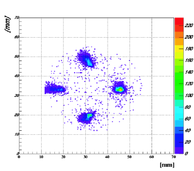
Figure 5: A two dimensional plot showing the x-y strip image of the four holes where the 5.9 keV X-rays go through during a calibration run.

3 Detector performance

3.1 Characterization

To characterize the detector a test was done at the PANTER X-ray facility of the Max-Planck-Institut für extraterrestrische Physik (MPE) in Munich [freyberg:06a]. A detector was mounted at the X-ray focusing telescope (now part of the CAST experiment) and tested with photon beams of varying energy. The detector, at the time, had a buffer space between the vacuum window and the detector drift electrode filled with Helium gas at atmospheric pressure. The buffer of Helium gas was used in order to couple the gaseous Micromegas volume at atmospheric pressure to the vacuum environment of the X-ray telescope (and of the CAST magnet bore) before the solution of the differential pumping was adopted. The drift space was 18 mm wide and the amplification gap was 50 $\mu$m. The X-Y position determination capability was for the first time shown and the remarkable agreement with the beam shape expected from the focusing properties of the X-ray telescope exhibited [andriamonje:04f]. Figure 6 shows a photo of the experimental set up as well as the logarithmic intensity plot of the X-Y position of 4.5 keV photons at the focus. The mm size core of the beam is clearly visible.

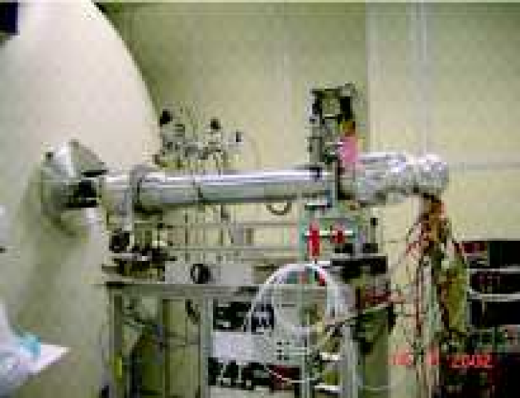
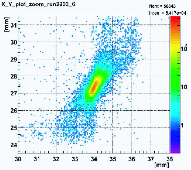
Figure 6: Left: Photo of the Micromegas detector mounted in the focal plane of the X-ray telescope at the PANTER facility. Right: Transverse position of the 4.5 keV focused photon beam at PANTER.

The efficiency of the detector was simulated using the GEANT4 package [geant4]. The dimensions of the detector, the materials of the windows (drift and helium buffer), the gas mixture as well as the beam spot were taken into account. In figure 7 the simulated efficiency with the experimental measured points is shown. The agreement observed allow us to use this simulation with slightly different parameters (drift space or window thickness) for the detectors that were used in the data taking periods.

Figure 7: Simulated detector efficiency as a function of energy with the experimental points measured at PANTER.

3.2 The 2003 detector

The Micromegas detector used for the 2003 data taking was designed with a 25 mm drift space and $50\,\mu{\rm m}$ amplification gap is formed by the help of kapton pillars on the micromesh plane. The detector accumulated data from May to mid-November without incident. For the last three months of data taking, the MATACQ card was installed allowing the recording of the pulse structure of the mesh pulse. An example of a calibration run is given in figure 8 where an energy resolution of 16% (FWHM) is obtained at 5.9 keV. The energy resolution obtained with the strips is about 30%. This degraded performance was due to some crosstalk between the strips caused by residual copper left on the kapton pillars of the micromesh which when in contact with the copper strips of the readout plane gave rise to this crosstalk.

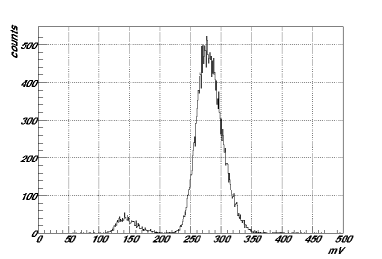
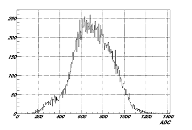
Figure 8: Energy spectrum for a calibration run using a ⁵⁵Fe source obtained with the mesh signal read by the MATACQ card (left) and with the strips (right).The energy resolution obtained with the strips is degraded due to residual crosstalk between the strips.

The detector’s linearity was verified by using a ¹⁰⁹Cd source which produced fluorescence of the detector’s material at different energies. Figure 9 shows the energy spectra as well as the linearity. The system was extremely stable: the time characteristics and energy response of the mesh pulses showed less than a 2% variation during the entire period.

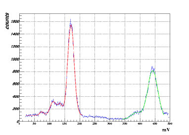
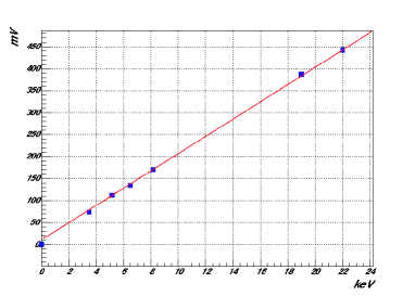
Figure 9: On the left energy spectra obtained with a Cd Source. Peaks at 8 keV due to the fluorescence of the Copper and the Cd 22 keV peak can be seen. On the right, the linearity plot showing the pulse height as a function of energy.

The Micromegas detector records tracking data at sunrise, and during the rest of the day background data is taken. The detector is calibrated daily. Signal events (photons with energy of $1$-$8\,\rm{keV}$) have a well defined signature giving a typical cluster in the read out strips and a typical pulse in the micromesh. Background events, coming from cosmic rays and natural radioactivity, give a bigger cluster in the strips, and the pulse shape in the micromesh is very different, favouring an efficient rejection based on the micromesh pulse shape and on the cluster topology. The offline analysis was based on sequential cuts, mainly on the micromesh pulse observables and less on the clustering (due to the strip crosstalk). Figure 10 shows the energy spectra for background events after the sequential cuts where the average background rate is $1.4\times 10^{-4}\,{\rm counts}\,{\rm cm}^{-2}\,{\rm s}^{-1}\,{\rm keV}^{-1}$ region. The background is composed of events coming from cosmic rays, natural radioactivity and fluorescence from materials present in the detector. The most visible peak is at 8 keV due to the Copper present in the anode plane as well as in the mesh cathode. The efficiency is defined as the ratio of the number of events that pass sequential cuts over the number of initial reconstructed events before cuts. This efficiency was calculated using the daily calibration runs giving 80% and 95% for 3 keV and 5.9 keV respectively.

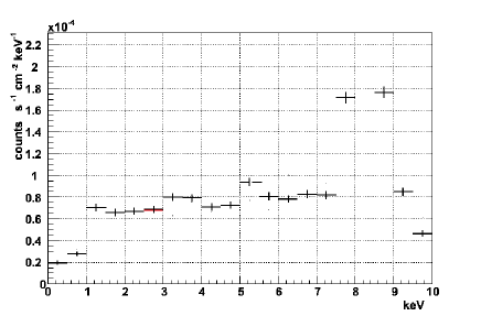
Figure 10: Background spectra after the filtering cuts for the 2003 data.

3.3 The 2004 detector

The experience acquired during the 2003 run led to the development of the V4 model with $30\,$mm conversion gap and $100\,\mu$m amplification gap, which was designed to eliminate the ”crosstalk” effects present at the previous model and to improve the quality of the strips. Both goals were achieved and moreover a faster MATACQ board was installed, reducing the detector’s dead time to 14 msec (less than 1.5% of the net data rate) while the energy resolution was 19% FWHM at 5.9 keV. The spectra obtained with the mesh signal recorded by the MATACQ card (left) and with the strips (right) are shown in figure 11. The energy resolution obtained with the mesh signal or with the strips is equally good for this detector due to the reduction of the strips crosstalk.

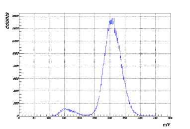
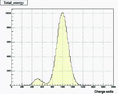
Figure 11: Energy spectrum for a calibration run using a ⁵⁵Fe source obtained with the mesh signal read by the MATACQ card (left) and with the strips (right). The energy resolution is less than 20% (FWMH) using both signals.

The very accurate strip data allowed us to improve the offline analysis dramatically by combining the information from the spatial distribution of the charge collected during an event with the time structure of the mesh pulses. More specifically, six observables (pulse risetime, pulse width, pulse height vs pulse integral correlation, X and Y strip multiplicity balance, X and Y strip charge balance, pulse height vs total strip charge correlation) were used in a modified Fisher discriminant method to distinguish more efficiently the proper X-ray events from other signals. Figure 12 shows the resulting background rejection to be at the level of $4.8\times 10^{-5}\,{\rm counts}\,{\rm cm}^{-2}\,{\rm s}^{-1}\,{\rm keV}^{-1}$ region with 94% uniform software efficiency. The system’s stability is demonstrated through the mesh pulses’ time structure (0.5% variation of risetime and width during the six months of the run) and the moderate gain variation (10% on a weekly base) which was corrected with daily calibration.

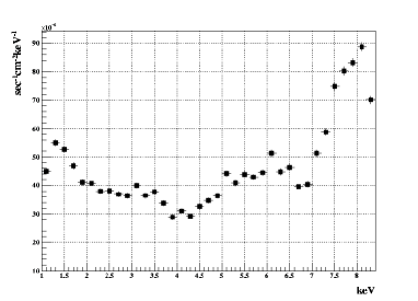
Figure 12: Background spectra after applying the Fisher discriminant method for analysis of the 2004 data andriamonje:07asee.

4 Conclusion

A Micromegas detector with novel features, such as the X-Y strip readout and the low background materials, was designed and constructed for the detection of $1$–$10\,{\rm keV}$ X-ray photons for the solar axion search experiment CAST at CERN. The excellent stability, linearity, position determination capability, low threshold and good energy resolution are shown. The analysis of the events permits the rejection of a large fraction of cosmic ray related background using the observed properties of genuine photon events such as the rise time and width of the micromesh signal, the cluster size and the X-Y energy balance. The best background rejection obtained has been shown to be at the level of $5\times 10^{-5}\,{\rm counts}\,{\rm cm}^{-2}\,{\rm s}^{-1}\,{\rm keV}^{-1}$ with an efficiency of 92%. With an appropriate shielding the rejection factor should easily be improved. This Micromegas design has produced a powerful device for the detection of X-rays from axions in the energy range of 1-10 keV. The achieved background rejection opens up the use of the Micromegas detector for other rare event searches.

References

References

-
[1]
\harvarditemAgostinelli et al.2003geant4
Agostinelli S, Allison J, Amako K, Apostolakis J, Araujo H, Arce P, Asai M,
Axen D, Banerjee S, Barrand G, Behner F, Bellagamba L, Boudreau J, Broglia L,
Brunengo A, Burkhardt H, Chauvie S, Chuma J, Chytracek R, Cooperman G, Cosmo
G, Degtyarenko P, dell’Acqua A, Depaola G, Dietrich D, Enami R, Feliciello A,
Ferguson C, Fesefeldt H, Folger G, Foppiano F, Forti A, Garelli S, Giani S,
Giannitrapani R, Gibin D, Gómez Cadenas J J, González I, Gracia Abril G,
Greeniaus G, Greiner W, Grichine V, Grossheim A, Guatelli S, Gumplinger P,
Hamatsu R, Hashimoto K, Hasui H, Heikkinen A, Howard A, Ivanchenko V, Johnson
A, Jones F W, Kallenbach J, Kanaya N, Kawabata M, Kawabata Y, Kawaguti M,
Kelner S, Kent P, Kimura A, Kodama T, Kokoulin R, Kossov M, Kurashige H,
Lamanna E, Lampén T, Lara V, Lefebure V, Lei F, Liendl M, Lockman W, Longo
F, Magni S, Maire M, Medernach E, Minamimoto K, Mora de Freitas P, Morita Y,
Murakami K, Nagamatu M, Nartallo R, Nieminen P, Nishimura T, Ohtsubo K,
Okamura M, O’Neale S, Oohata Y, Paech K, Perl J, Pfeiffer A, Pia M G, Ranjard
F, Rybin A, Sadilov S, di Salvo E, Santin G, Sasaki T, Savvas N, Sawada Y,
Scherer S, Sei S, Sirotenko V, Smith D, Starkov N, Stoecker H, Sulkimo J,
Takahata M, Tanaka S, Tcherniaev E, Safai Tehrani E, Tropeano M, Truscott P,
Uno H, Urban L, Urban P, Verderi M, Walkden A, Wander W, Weber H, Wellisch
J P, Wenaus T, Williams D C, Wright D, Yamada T, Yoshida H \harvardand Zschiesche D 2003 Nucl. Instrum. Methods Phys. Res., Sect. A 506, 250–303.
\harvardurlhttp://www.cern.ch/geant4 - [2] \harvarditemAndriamonje et al.2007andriamonje:07b Andriamonje S, Aune S, Autiero D, Barth K, Belov A, Beltrán B, Bräuninger H, Carmona J, Cebrián S, Collar J I, Dafni T, Davenport M, Di Lella L, Eleftheriadis C, Englhauser J, Fanourakis G, Ferrer Ribas E, Fischer H, Franz J, Friedrich P, Geralis T, Giomataris I, Gninenko S, Gómez H, Hasinoff M, Heinsius F H, Hoffmann D H H, Irastorza I G, Jacoby J, Jakovčić K, Kang D, Königsmann K, Kotthaus R, Krčmar M, Kousouris K, Kuster M, Lakić B, Lasseur C, Liolios A, Ljubičić A, Lutz G, Luzon G, Miller D, Morales A, Morales J, Ortiz A, Papaevangelou T, Placci A, Raffelt G, Riege H, Rodríguez A, Ruz J, Savvidis I, Semertzidis Y, Serpico P, Stewart L, Vieira J, Villar J, Vogel J, Walckiers L \harvardand Zioutas K 2007 New. J. Phys. in preparation.
- [3] \harvarditemAndriamonje et al.2007andriamonje:07a Andriamonje S, Aune S, Barth K, Belov A, Beltrán B, Bräuninger H, Carmona J, Cebrián S, Collar J I, Dafni T, Davenport M, Di Lella L, Eleftheriadis C, Englhauser J, Fanourakis G, Ferrer-Ribas E, Fischer H, Franz J, Friedrich P, Geralis T, Giomataris I, Gninenko S, Gómez H, Hasinoff M, Heinsius F H, Hoffmann D H H, Irastorza I G, Jacoby J, Jakovčić K, Kang D, Königsmann K, Kotthaus R, Krčmar M, Kousouris K, Kuster M, Lakić B, Lasseur C, Liolios A, Ljubičić A, Lutz G, Luzon G, Miller D, Morales A, Morales J, Ortiz A, Papaevangelou T, Placci A, Raffelt G, Riege H, Rodríguez A, Ruz J, Savvidis I, Semertzidis Y, Serpico P, Stewart L, Villar J, Vogel J, Walckiers L \harvardand Zioutas K 2007 J. Cosmol. Astropart. Phys. submitted.
- [4] \harvarditemAndriamonje et al.2004andriamonje:04f Andriamonje S, Aune S, Dafni T, Fanourakis G, Ferrer Ribas E, Fischer H, Franz J, Geralis T, Giganon A, Giomataris Y, Heinsius F H, Königsmann K, Papaevangelou T \harvardand Zachariadou K 2004 Nucl. Instrum. Methods Phys. Res., Sect. A 518, 252–255.
- [5] \harvarditemAutiero et al.2007autiero:06a Autiero D, Beltrán B, Carmona J M, Cebrián S, Chesi E, Davenport M, Delattre M, Di Lella L, Formenti F, Irastorza I G, Gomez H, Hasinoff M, Lakić B, Luzón G, Morales J, Musa L, Ortiz A, Placci A, Rodriguez A, Ruz J \harvardand Villar J A 2007 New. J. Phys. this volume.
- [6] \harvarditemBreton et al.n.d.breton:05a Breton D, Delagnes E \harvardand Houry M n.d. in ‘Trans. Nucl. Sci.’ Vol. 52 of IEEE p. 2853.
- [7] \harvarditemCharpak et al.2002charpak:02a Charpak G, Derré J, Giomataris Y \harvardand Rebourgeard P 2002 Nucl. Instrum. Methods Phys. Res., Sect. A 478, 26–36.
- [8] \harvarditemColas et al.2004colas:04a Colas P, Colijn A P, Fornaini A, Giomataris Y, van der Graaf H, Heijne E H M, Llopart X, Schmitz J, Timmermans J \harvardand Visschers J L 2004 Nucl. Instrum. Methods Phys. Res., Sect. A 535, 506–510.
- [9] \harvarditemCollar \harvardand Giomataris2000collar:00a Collar J \harvardand Giomataris Y 2000 Nucl. Instrum. Methods Phys. Res., Sect. A 471, 254.
- [10] \harvarditemDelbart et al.2001delbart:02a Delbart A, Oliveira R D, Derré J, Giomataris Y, Jeanneau F, Papadopoulos Y \harvardand Rebourgeard P 2001 Nucl. Instrum. Methods Phys. Res., Sect. A 461, 84–87.
- [11] \harvarditemFreyberg et al.2005freyberg:06a Freyberg M J, Bräuninger H, Burkert W, Hartner G D, Citterio O, Mazzoleni F, Pareschi G, Spiga D, Romaine S, Gorenstein P \harvardand Ramsey B D 2005 Experimental Astronomy 20, 405–412.
- [12] \harvarditemGeralis et al.2003Geralis:03a Geralis T, Fanourakis G, Giomataris Y \harvardand Zachariadou K 2003 in ‘Nuclear Science Symposium Conference Record – IEEE’ Vol. 5 pp. 3455–3499.
- [13] \harvarditemGiomataris et al.2006giomataris:06a Giomataris I, de Oliveira R, Andriamonje S, Aune S, Charpak G, Colas P, Fanourakis G, Ferrer E, Giganon A, Rebourgeard P \harvardand Salin P 2006 Nucl. Instrum. Methods Phys. Res., Sect. A 560, 405–408.
- [14] \harvarditemGiomataris1998giomataris:98a Giomataris Y 1998 Nucl. Instrum. Methods Phys. Res., Sect. A 419, 239–250.
- [15] \harvarditemGiomataris et al.1996giomataris:96a Giomataris Y, Rebourgeard P, Robert J P \harvardand Charpak G 1996 Nucl. Instrum. Methods Phys. Res., Sect. A 376, 29–35.
- [16] \harvarditemKuster et al.2007kuster:06a Kuster M, Bräuniger H, Davenport M, Englhauser J, Fischer H, Franz J, Friedrich P, Hartmann R, H. H F, Hoffmann D, Hoffmeister G, Joux J N, Kang D, Köningsmann K, Kotthaus, R. Papaevangelou T, Lasseur C, Lippitsch A, Lutz G, Strüder L, Vogel J \harvardand Zioutas K 2007 New J. Phys. this volume.
- [17] \harvarditemSantiard et al.1994Santiard:94a Santiard J C, Beusch W, Buytaert S, Enz C, Heijne E, Jarron P, Krummenacher F, Marent K \harvardand Piuz F 1994. Presented at the 6th Pisa Meeting on Advanced Detectors, La Biodola, Isola d’Elba, Italy, 22 - 28 May 1994, CERN-ECP-94-17.
- [18] \harvarditemZioutas et al.2005zioutas:05a Zioutas K, Andriamonje S, Arsov V, Aune S, Autiero D, Avignone F T, Barth K, Belov A, Beltrán B, Bräuninger H, Carmona J M, Cebrián S, Chesi E, Collar J I, Creswick R, Dafni T, Davenport M, di Lella L, Eleftheriadis C, Englhauser J, Fanourakis G, Farach H, Ferrer E, Fischer H, Franz J, Friedrich P, Geralis T, Giomataris I, Gninenko S, Goloubev N, Hasinoff M D, Heinsius F H, Hoffmann D H H, Irastorza I G, Jacoby J, Kang D, Königsmann K, Kotthaus R, Krčmar M, Kousouris K, Kuster M, Lakić B, Lasseur C, Liolios A, Ljubičić A, Lutz G, Luzón G, Miller D W, Morales A, Morales J, Mutterer M, Nikolaidis A, Ortiz A, Papaevangelou T, Placci A, Raffelt G, Ruz J, Riege H, Sarsa M L, Savvidis I, Serber W, Serpico P, Semertzidis Y, Stewart L, Vieira J D, Villar J, Walckiers L \harvardand Zachariadou K 2005 Phys. Rev. Lett. 94(12), 121301–+.
- [19]