A Toy Model of the Rat Race

Abstract

We introduce a toy model of the “rat race” in which individuals try to better themselves relative to the rest of the population. An individual is characterized by a real-valued fitness and each advances at a constant rate by an amount that depends on its standing in the population. The leader advances to remain ahead of its nearest neighbor, while all others advance by an amount that is set by the distance to the leader. A rich dynamics occurs as a function of the mean jump size of the trailing particles. For small jumps, the leader maintains its position, while for large jumps, there are long periods of stasis that are punctuated by episodes of explosive advancement and many lead changes. Intermediate to these two regimes, in a typical realization of the system, agents reach a common fitness and evolution grinds to a halt.

I INTRODUCTION

A basic fact of life is competition. In evolution, only the fittest survive; in the workplace, we compete for professional advancement; in social events, we compete for attention; in sports, its very purpose is to excel in competition. Idealized models of social competition have recently been proposed in which the status of each individual is determined by competitive success btd ; br ; bvr ; msk . In this spirit, we introduce a simple “rate-race” model that embodies the struggle for advancement in a competitive environment. Because everyone is engaged in the same perpetual rat race, one’s relative standing may change slowly or not at all, even though the population as a whole may be advancing. When the competition favors the strong, the leader runs away from the rest of the population. As the competition becomes more equitable, in any typical realization of the system, everyone reaches the same fitness and the population become static. When the leader is easily overtaken, the mean fitness undergoes periods of near stasis and explosive advancement that qualitatively mirrors the phenomenon of punctuated evolution punc .

Empirical motivations for our model come from evolution and from sports. In evolution, large-scale species extinctions occur during sudden spurts, with much slower development during the intervening periods punc ; evol . These periods of near stasis characterize many sports, where it is not possible to maintain a long-term competitive advantage. If one finds such a winning strategy, competitors will eventually find a counter-strategy so that any advantage is lost. Conversely, a consistent loser will be replaced by a more competent individual so that losing strategies also do not persist.

A famous example of the latter idea comes from baseball, where the mythic achievement of a .400 hitter, an exceptional player who gets a hit in more than 40% of his turns at bat, occurred multiple times during the early years of the sport—25 times from 1871 to 1941 (last accomplished by the .406 batting average of Ted Williams of the Boston Red Sox in 1941)—but none since then. An appealing explanation for this phenomenon, proposed by S. J. Gould G , is that the increasing competitiveness as the sport has developed makes outliers less likely to occur. To illustrate this point, Gould found that the dispersion in the batting averages of all regular players decreased systematically from 1875 until 1980, even though year-to-year fluctuations in their mean batting average are larger than the systematic decrease in the dispersion. Thus outliers become rarer and exceptional achievements, such as a season batting average over .400, or a consecutive-game hitting streak longer than 56 achieved by Joe DiMaggio also in 1941, should not recur.

In the next section, we define the rat race model and then we analytically determine its dynamical features for a two-agent system in Sec. III. In Sec. IV, we investigate many agents in the framework of an almost deterministic version of the rat race. Simulation results for the evolutionary behavior of the model are given in Sec. V, and we conclude in Sec. VI.

II RAT RACE MODEL

In our rat race model, each individual $i=0,1,2,\ldots$ possesses a real-valued fitness $x_{i}$, with larger $x_{i}$ representing higher fitness (Fig. 1). An individual attempts to improve with respect to the competition by advancing to larger $x$. Advancement events occur one at a time and each individual has the same rate of advancing; i.e., we consider serial dynamics in which a randomly-selected competitor advances. The leader, located at $x_{0}$, advances by an amount that is drawn from a uniform distribution of width $x_{0}-x_{1}$. That is, the leader is aware only of the next strongest individual and attempts to maintain its lead by advancing by an amount that is of the order of the separation to this nearest neighbor. On the other hand, all other individuals seek to overtake the leader. The $i^{\rm th}$ agent, with fitness $x_{i}$, moves a distance that is uniformly distributed in the range $m(x_{0}-x_{i})$. Here $m$ is the fundamental parameter—the “catch-up” factor—that quantifies the severity of the competition. When $m<1$, the leader maintains the lead forever, while for $m>1$ the leader can be overtaken.

Figure 1: Stochastic rat race model. Each particle has a fitness $x_{k}$. The leader can advance by an amount that is uniformly distributed in the range $x_{0}-x_{1}$. The $k^{\rm th}$ particle can advance by an amount that is uniformly distributed in $m(x_{0}-x_{k})$.

In the context of competition, it would be more realistic to eliminate laggards and replace them by typical individuals. However, our model mimics precisely this situation, as a laggard typically moves toward the average fitness. A lazy population is characterized by a small value of $m$ for which the leader maintains the lead on the rest of the pack. For a sufficiently large value of $m$, however, the lead changes often and by large amounts so that the width of the fitness distribution increases after each advancement event. Between these two extremes there is an intermediate regime of stasis where the spread of the pack shrinks to zero and the population stops advancing.

III TWO COMPETITORS

We begin by studying the case of two agents with fitnesses $x_{0}$ and $x_{1}<x_{0}$ and gap $g=x_{0}-x_{1}$. The fitness of the leader increases by an amount that is uniformly distributed in $[0,g]$ to try to maintain its lead. Similarly, the laggard advances by a distance that is uniformly distributed in the range $[0,mg]$. For $m<1$ the agents always maintain their order, while for $m>1$ lead changes can occur. We now determine the evolution of the gap length for any $m$.

The gap length undergoes a random multiplicative process because each advancement step leads to a multiplicative change. Thus we expect that the distribution of gap lengths for an ensemble of two-agent systems will have a log-normal form. Additionally, over a suitable range for the catch-up factor $m$ we also expect large fluctuations between different realizations of the process, as is well-known to occur in random multiplicative processes rmp .

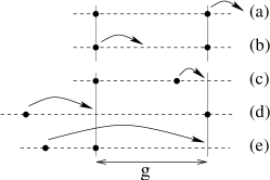
Figure 2: Advancement events that contribute to the change in the gap length for a two-particle rat race. Gaps of length $g$ are lost by the first two process, while the latter three lead to a gain of gaps of length $g$. The last process is a lead-changing event.

III.1 Gap Evolution

The gap evolution is completely described by $P(g,t)$, the probability for a gap of length $g$ at time $t$. For the case $m<1$ (no lead changes), the evolution of $P$ is described the master equation

$$\begin{split}\dot{P}(g)&=-P(g)+\frac{1}{2}\int_{\frac{g}{2}}^{g}\frac{P(g^{\prime})}{g^{\prime}}\,dg^{\prime}\\ &~{}~{}~{}~{}~{}~{}~{}~{}~{}~{}~{}~{}~{}~{}~{}~{}~{}~{}+\frac{1}{2m}\int_{g}^{\frac{g}{1-m}}\frac{P(g^{\prime})}{g^{\prime}}\,dg^{\prime}\,,\end{split}$$ (1)

where the overdot denotes time derivative. The first term on the right accounts for the loss of gaps of length $g$ because of the hopping of either particle ((a), (b) in Fig. 2). The second term accounts for the creation of a gap of length $g$ due to the leader advancing from a previous gap of length $g^{\prime}<g$ (Fig. 2(c)). The length $g^{\prime}$ of this previous gap must be in the range $[g/2,g]$ so that a gap of length $g$ can be created and the factor $1/g^{\prime}$ accounts for the hopping distance being uniformly distributed in $[0,g^{\prime}]$. The last term accounts for the laggard advancing to create a gap of length $g$ (Fig. 2(d)). Here, the previous gap length $g^{\prime}$ must be in the range $[g,g/(1-m)]$ and the hopping probability then equals $1/(mg^{\prime})$.

Similarly, the master equation for $P(g)$ for $m>1$ is:

$$\begin{split}\dot{P}(g)&=-P(g)+\frac{1}{2}\int_{\frac{g}{2}}^{g}\frac{P(g^{\prime})}{g^{\prime}}\,dg^{\prime}\\ &~{}~{}~{}~{}~{}~{}+\frac{1}{2m}\int_{g}^{\infty}\frac{P(g^{\prime})}{g^{\prime}}\,dg^{\prime}+\frac{1}{2m}\int_{\frac{g}{m-1}}^{\infty}\frac{P(g^{\prime})}{g^{\prime}}\,dg^{\prime}\,.\end{split}$$ (2)

The third term on the right accounts for events in which the laggard remains the laggard (Fig. 2(d)), while the last term accounts for overtaking events (Fig. 2(e)).

For both $m<1$ and $m>1$, it is straightforward to check that these equations conserve the total probability, $\int_{0}^{\infty}\dot{P}(g)\,dg=0$. For this purpose, we need to compute

$$\int_{0}^{\infty}\dot{P}(g)\,dg=\int_{0}^{\infty}\big{[}\cdots]\,dg$$ (3)

where $[\cdots]$ denotes the right-hand side of Eq. (1) or Eq. (2). To perform this type of integral, we merely interchange the order of the $g$ and $g^{\prime}$ integrations. We illustrate this calculation for the second term on the right-hand side of Eq. (1). The interchange of integration order in this term gives

$$\int_{0}^{\infty}dg\,\,\frac{1}{2}\int_{g/2}^{g}\frac{P(g^{\prime})}{g^{\prime}}dg^{\prime}=\frac{1}{2}\int_{0}^{\infty}dg^{\prime}\int_{g^{\prime}}^{2g^{\prime}}\frac{P(g^{\prime})}{g^{\prime}}\,dg$$

The integration over $g$ merely gives $g^{\prime}$ and then the $g^{\prime}$ integral becomes simply $\frac{1}{2}\int_{0}^{\infty}P(g^{\prime})\,dg^{\prime}=\frac{1}{2}$. The same manipulation works for all the other terms in the master equation and we thus verify that $\int P(g)\,dg$ is conserved.

III.2 Moments of the Gap Length

The equation of motion for the moments of the gap-length distribution is

$$\dot{\mathcal{M}_{k}}\equiv\left\langle\frac{dg^{k}}{dt}\right\rangle=\int_{0}^{\infty}g^{k}\dot{P}(g)\,dg=\int_{0}^{\infty}g^{k}\,\big{[}\cdots]\,dg\,,$$ (4)

where $[\cdots]$ again denotes the right-hand side of Eq. (1) or Eq. (2). Employing the same interchange of integration order as illustrated above, the integrals can be evaluated straightforwardly to yield the following closed equations for the moments:

$$\dot{\mathcal{M}_{k}}=\mathcal{M}_{k}\!\times\!\begin{cases}{\displaystyle-1+\frac{2^{k+1}\!-\!1}{2(k+1)}+\frac{1-(1\!-\!m)^{k+1}}{2m(k+1)}}&m<1;\\ \\ {\displaystyle-1+\frac{2^{k+1}\!-\!1}{2(k+1)}+\frac{(m\!-\!1)^{k+1}+1}{2m(k+1)}}&m>1.\end{cases}$$ (5)

For $m<1$, the first few moments obey:

$$\dot{\mathcal{M}}_{0} = 0$$

$$\dot{\mathcal{M}_{1}} = \mathcal{M}_{1}\left(\frac{1-m}{4}\right)$$

$$\dot{\mathcal{M}_{2}} = \mathcal{M}_{2}\left(\frac{3-2m+m^{2}}{6m}\right)$$ (6)

etc. All positive integer moments increase in time for $m<1$ because the leader hops further than the laggard, on average, in every single event. Conversely, for $m>1$ the corresponding moment equations are:

$$\dot{\mathcal{M}_{0}} = 0$$

$$\dot{\mathcal{M}_{1}} = \mathcal{M}_{1}\left[\frac{(m-1)(m-2)}{4m}\right]$$

$$\dot{\mathcal{M}_{2}} = \mathcal{M}_{2}\left[\frac{(m-1)^{3}+m+1}{6m}\right]$$ (7)

etc. Curiously, different moments can have opposite time dependences. For $m<1$ the laggard trails further and further behind after each step and the average separation grows, while for $m>2$, overtaking events are so drastic in character that the average separation between the two agents also grows. Conversely, for $1<m<2$, the first moment decreases in time. In spite of the differing behaviors for the first moment as a function of $m$, higher moments grow for any $m>1$ (Eq. (III.2)).

Why does this dichotomy between moments of different order arise? The source is the multiplicative process that underlies the gap dynamics. This multiplicativity leads to the very broad log-normal distribution of gap sizes (to be derived in the next section), for which the time dependence of moments of different order can be quite different rmp . In a random multiplicative process, extreme realizations with an exponentially small probability, make an exponentially large contribution to the moment of a given order. For $m<1$ or $m>2$, the interplay between these two extremes leads to a first moment that grows with time when summing over all realizations. In simulations, however, we study only a small fraction of all realizations and thus can observe only the very different most probable behavior.

The most probable gap $g_{\rm mp}=e^{\langle\ln g\rangle}$ (the geometric average of $g$) may be obtained by computing $\dot{X}\equiv\langle\dot{\ln}g\rangle$, using the same approach that leads from Eq. (4) to (5). We thereby find that $X=At$ with

$$A=\begin{cases}{\displaystyle\ln 2-1+\frac{(m-1)\ln(1-m)}{2m}}&m<1;\\ \\ {\displaystyle\ln 2-1+\frac{(m-1)\ln(m-1)}{2m}}&m>1.\end{cases}$$ (8)

Setting $A=0$ gives the transition at which the most probable gap length does not change. Again there are two transitions; from the first line of (8), the condition $A=0$ gives a transcendental equation for $m$ with solution $m_{1}^{*}=0.596754\ldots$. Similarly, from the second line of (8), the condition $A=0$ gives the threshold $m_{2}^{*}=3.38846\ldots$. The most probable gap length $g_{\rm mp}$ thus increases with time for $m<m_{1}^{*}$ and $m>m_{2}^{*}$, while $g_{\rm mp}$ shrinks to zero in a finite time for $m_{1}^{*}<m<m_{2}^{*}$. Comparing Eqs. (III.2) & (8), there exists a range of $m$ for which the average gap grows while the most probable gap shrinks. Again, the interplay between exponentially unlikely events that have exponentially large contributions to an observable gives seemingly contradictory results that are natural outcomes of a random multiplicative process rmp .

III.3 The Gap Length Distribution

We now compute the asymptotic tails of the gap length distribution itself. Our approach to determine this distribution is to write the moments of the gap length distribution in Eqs. (5) as a Fourier transform and then invert this transform.

Thus we write

$$\int_{0}^{\infty}P(g,t)\,g^{k}\,dg=e^{\ln[\mathcal{M}_{k}(t)]}\,.$$

Now define $X=\ln g$ and make an analytic continuation from $k$ to $ik$ to give

$$\int_{-\infty}^{\infty}P(X,t)\,e^{ikX}\,dX=e^{\ln[\mathcal{M}_{ik}(t)]}\,.$$

The left-hand side is just the Fourier transform of $P(X,t)$. Inverting this Fourier transform, we obtain

$$P(X,t)=\frac{1}{2\pi}\int_{-\infty}^{\infty}dk\,\,e^{-ikX}\,e^{\ln[\mathcal{M}_{ik}(t)]}\,.$$

To derive the asymptotic distribution for large $X$, we need the small-$k$ behavior of $\ln\mathcal{M}_{ik}$. Using (5), we expand $\ln\mathcal{M}_{ik}$ for small $k$ and then invert the Fourier transform to obtain a Gaussian distribution for $X$, i.e., a log-normal distribution for $g$. The final result is

$$P(X,t)\sim\frac{1}{\sqrt{2\pi Bt}}\,e^{-(X-At)^{2}/{2Bt}}\,,$$ (9)

where $A$ is given by Eq. (8) and

$$B=\begin{cases}C-\frac{m-1}{2m}\left[2\ln(1-m)-\ln^{2}(1-m)\right]&m<1\\ \\ C-\frac{m-1}{2m}\left[2\ln(m-1)-\ln^{2}(m-1)\right]&m>1,\end{cases}$$ (10)

with $C=2-2\ln 2+(\ln 2)^{2}$. We again emphasize that while the distribution of $X=\ln g$ extends over range that grows as $\sqrt{t}$, the distribution of $g$ itself is extremely broad so that it cannot be characterized by any individual moment.

IV DETERMINISTIC MODEL

It is not clear how to adapt the theory given above in an analytically-tractable way to treat more than 2 particles. We therefore introduce an nearly-deterministic version of the model that mimics the advancement steps in the stochastic rat race model by defining the length of each jump to be exactly one half of the total possible range. We again consider serial dynamics in which one of the competitors, chosen at random, advances. The order in which competitors are selected is the only source of stochasticity in this version of the model.

IV.1 Two Particles

There are two possibilities for particle movement, depending on the value of the catch-up factor $m$:

• For $m<2$, if the leader moves, the gap $g\to(3/2)g$, while if the laggard moves, the gap $g\to\beta g$, where $\beta=1-(m/2)$.

• For $m>2$ the laggard overtakes the leader. If the leader moves, again $g\to(3/2)g$, while if the laggard moves $g\to\beta g$, where $\beta=(m/2)-1$.

Since either particle is selected with probability 1/2 at each step, after $t$ steps the gap could assume any of the values $(3/2)^{\tau}\beta^{t-\tau}$, $\tau=0,1,\dots,t$ (assuming an initial gap length $g=1$). After $t$ steps, the probability of a gap of length $(3/2)^{\tau}\beta^{t-\tau}$ is

$$p_{\tau}=\frac{1}{2^{t}}\Big{(}{t\atop\tau}\Big{)}\,.$$

Figure 3: Deterministic rat race. The laggard advances by $mg/2$. For $m<2$, the order never changes, while for $m>2$, the move of the laggard always leads to passing.

It follows that the $k^{\rm th}$ moment of the gap length is

$$\mathcal{M}_{k}\equiv\langle g^{k}\rangle=\Big{[}\frac{1}{2}\Big{(}\frac{3}{2}\Big{)}^{k}+\frac{1}{2}\beta^{k}\Big{]}^{t}\,.$$ (11)

Thus, the large-time behavior of the $k^{\rm th}$ moment depends on the factor $[(3/2)^{k}+\beta^{k}]/2$. If this factor is greater than $1$, i.e., $\beta$ exceeds $\beta_{c}(k)=\exp[\ln(2-(3/2)^{k})/k]$, the $k^{\rm th}$ moment diverges as $t\to\infty$. On the other hand, for $\beta<\beta_{c}(k)$, the $k^{\rm th}$ moment vanishes as $t\to\infty$. For $\beta>\beta_{c}(0)=2/3$, all positive moments of the gap size, as well as the most probable gap size, diverge. The value $\beta_{c}(0)=2/3$ thus marks the transition from convergent to explosive behavior in the gap size. Notice that this transition value for $\beta$ corresponds to the threshold values $m_{1}^{*}=2/3$ and $m_{2}^{*}=10/3$, which agree well with the corresponding thresholds from the stochastic rat race.

IV.2 Many Particles

We study an $N+1$-particle system, with $N>1$, with particles located at $x_{i}$, with $i=0,1,2,\ldots N$. The gap between particle $n$ and the leader is defined as $g_{n}=x_{0}-x_{n}$. We limit ourselves to the case of catch-up factor $m>2$, so that any non-leader that jumps always overtakes the leader. This fact allows us to keep track of the ordering of the particles and an exact analysis is then possible. For generality, we assume the leader jumps a distance $\alpha g_{1}$ ahead; $\alpha=1/2$ corresponds to the case analyzed previously, while for $\alpha=0$ the leader is completely lazy and never jumps.

If particle $n$ is selected, this results in a re-distribution of the vector $(g_{1},g_{2},\dots,g_{N})$ of the gap lengths:

$${\bf g}^{\prime}={\bf A}_{n}{\bf g}\,,$$

where

$${\bf A}_{0}=\left(\begin{array}[]{ccccc}1+\alpha&0&0&\cdots&0\\ 1-\alpha&1&0&\cdots&0\\ 1-\alpha&0&1&\cdots&0\\ \vdots&\vdots&\vdots&\ddots&\vdots\\ 1-\alpha&0&0&\cdots&1\end{array}\right),\>{\bf A}_{1}=\left(\begin{array}[]{ccccc}\beta&0&0&\cdots&0\\ \beta&1&0&\cdots&0\\ \beta&0&1&\cdots&0\\ \vdots&\vdots&\vdots&\ddots&\vdots\\ \beta&0&0&\cdots&1\end{array}\right),$$

$${\bf A}_{2}=\left(\begin{array}[]{ccccc}0&\beta&0&\cdots&0\\ 1&\beta&0&\cdots&0\\ 0&\beta&1&\cdots&0\\ \vdots&\vdots&\vdots&\ddots&\vdots\\ 0&\beta&0&\cdots&1\end{array}\right),\dots\>{\bf A}_{N}=\left(\begin{array}[]{ccccc}0&0&0&\cdots&\beta\\ 1&0&0&\cdots&\beta\\ 0&1&0&\cdots&\beta\\ \vdots&\vdots&\ddots&&\vdots\\ 0&0&\cdots&1&\beta\end{array}\right).$$

The vector g, after $t$ steps, is the result of the product of $t$ matrices, drawn at random from among the ${\bf A}_{n}$. Unfortunately, none of the matrices commute, so we cannot deduce the probability distribution of gap sizes as in the scalar case of two particles ($N=1$). On the other hand, according to the Oseledec theorem O (also known as the multiplicative ergodic theorem), the growth of g is determined by the product ${\tilde{\lambda}}_{0}{\tilde{\lambda}}_{1}\cdots{\tilde{\lambda}}_{N}$, where ${\tilde{\lambda}}_{n}$ is the largest eigenvalue of the matrix ${\bf A}_{n}$ ($n=0,1,2,\dots N$). More precisely, the product $\mathcal{P}\equiv\prod_{i=0}^{N}\tilde{\lambda}_{i}$ determines the largest Lyapunov exponent of the growth of g with $N$. Thus explosive growth results if the product $\mathcal{P}>1$, and stasis results otherwise. We now derive the critical value for $\beta$ at the transition point, where ${\tilde{\lambda}}_{0}{\tilde{\lambda}}_{1}\cdots{\tilde{\lambda}}_{N}=1$.

The largest eigenvalue of ${\bf A}_{0}$ is clearly ${\tilde{\lambda}}_{0}=1+\alpha$. To determine the largest eigenvalue of ${\bf A}_{n}$ for $n>0$, we write the characteristic equation det$({\bf A}_{n}-\lambda{{\bf I}})=0$, obtained by expanding the determinant about the column of $\beta$’s:

$$[\beta(1+\lambda+\lambda^{2}+\cdots+\lambda^{n-1})-\lambda^{n}](1-\lambda)^{N-n}=0\,.$$

From the second factor on the left-hand side we conclude that ${\bf A}_{n}$ has $N-n$ eigenvalues $\lambda_{n}=1$. We argue, self-consistently, that for $n=1,2,\dots,N-1$ these are also the largest eigenvalues, that is, ${\tilde{\lambda}}_{n}=1$. Indeed, if that is the case, then the criticality condition dictates ${\tilde{\lambda}}_{N}=1/(1+\alpha)$. Substituting this value into the characteristic equation for ${\bf A}_{N}$ we find

$$\beta^{*}=\frac{\alpha}{(1+\alpha)^{N+1}-(1+\alpha)}\,.$$ (12)

It follows that $\beta^{*}\leq 1/N$ (with the equality being realized in the limit $\alpha\to 0$). We can now show that our initial assumption that the remaining eigenvalues of ${\bf A}_{n}$ ($n=1,2,\dots,N-1$) are not larger than 1 is indeed valid. From the factor in the square brackets of the characteristic equation, we see that these eigenvalues satisfy

$$\beta=\frac{\lambda^{n}}{1+\lambda+\lambda^{2}+\cdots+\lambda^{n-1}}\,.$$

The expression on the right-hand side is a monotonically increasing function of $\lambda$, hence if $\lambda>1$ then $\beta>1/n>1/N$, in contradiction with (12).

For $\alpha=0$, namely, the case of a lazy leader that never advances as long as it leads, the critical value of the catch-up parameter $\beta$ is no longer exponential in $N$, but rather

$$\beta^{*}=\frac{1}{N}\,,$$ (13)

as can be seen by taking the limit of $\alpha\to 0$ in Eq. (12).

V SIMULATION RESULTS

For any number of agents, the time dependence of the fitness of each agent exhibits rich behavior. For 2 agents, simulations clearly show a transition between a regime where the leader runs away from the laggard and stasis as $m$ passes through a critical value close to $m_{1}^{*}=0.596754\ldots$. This stasis continues until a second transition at $m\approx m_{2}^{*}=3.38846\ldots$. For $m>m_{2}^{*}$, there is explosive growth, with many lead changes between the two agents. It bears emphasizing that the observed transitions occur close to the values associated with the most probable gap size, even though the true transitions occur at $m_{1}=1$ and $m_{2}=2$, corresponding to the average gap size. Since simulations reflect the most probable behavior, they can provide qualitative information about the nature of stasis and explosive growth, as well as the transition between these two regimes, but little else.

Figs. 4 and  5 show typical results for 6 agents. Again, the existence of two transitions is clearly visible. For $m<m_{1}^{*}\approx 0.4$, the initial leader always maintains its lead, but the laggards are able to remain relatively close behind by virtue of the multiplicative nature of the jumps. Strikingly, large jumps occur with some frequency so that the population still advances rapidly. However, for slightly larger $m$, the distance between the strongest and weakest eventually disappears and the evolution quickly grinds to a halt (Fig. 4 bottom). Here lead changes are rare and no longer occur after a short time. This nearly static behavior continues until $m\approx 1.6$ (Fig. 5 top).

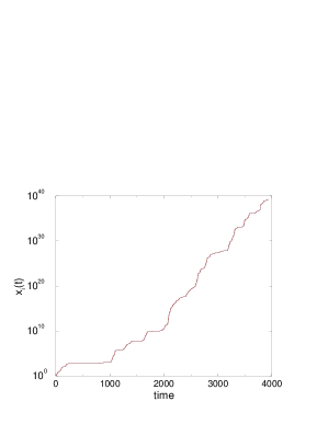
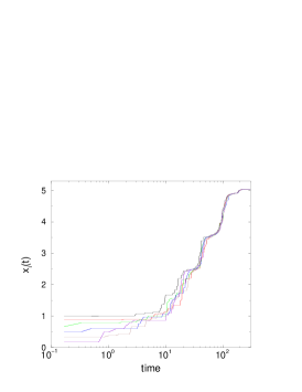
Figure 4: Fitnesses of each agent for a 6-particle system for $m=0.4$ on a linear-log scale (top), and $m=0.44$ on a log-linear scale (bottom).

For a slightly larger $m$, this system exhibits periods of near stasis followed by periods of explosive growth (Fig. 5 bottom). Here lead changes occur at roughly a constant rate and the total number of lead changes grows linearly with time. During periods of rapid advancement, the gap between the strongest and weakest agent is nearly comparable to the fitness (position) of any agent. Conversely, during periods of near stasis, the gap between the strongest and weakest agent is orders of magnitude smaller than the typical fitness.

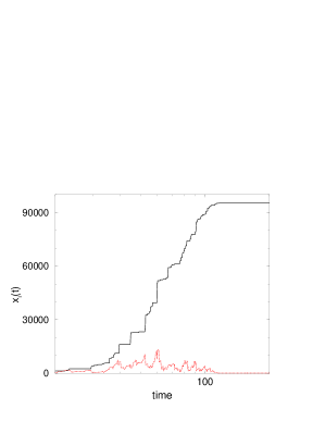
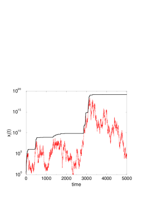
Figure 5: Fitnesses of each agent for a 6-particle system for $m=1.61$ on a log-linear scale (top) and $m=1.64$ on a linear-log scale (bottom). Shown dotted is the distance between the strongest and weakest agent.

Qualitatively similar behavior occurs for more particles, except that the critical values of $m$ that separates leader runaway from stasis and stasis from explosive growth seem to approach 0 and 1, respectively, as the number of particles increases.

VI SUMMARY

We introduced an idealized social competition model where individuals try to better their fitness (a real-valued variable) by advancing relative to the rest of the population: the leader advances to remain ahead of its closest pursuer, while others in the pack advance by a random amount, in proportion to their distance from the leader. When this proportionality constant is too small or too large, the fitness of all the agents grows explosively during short sporadic bursts. These explosive regimes are the analog of the rapid growth of new species after massive die-offs in punctuated evolution. Between these two extremes there is a window of stasis, where the spread of the pack shrinks indefinitely and evolution comes to a stop. Here outliers becomes progressively less likely and extreme achievements disappear; this situation parallels the disappearance of the .400 hitter in baseball mentioned in the introduction.

Basic features of the model already arise in the simple limits of just two agents, and in a deterministic model where agents advance by a fixed multiple of their gap to the leader. These simplified models allow for an exact analysis, yielding specific expressions for the distribution of gaps in the two-agent model, and for the $N$-dependence of the threshold parameters that demarcate between the regimes of stasis and explosive growth in the deterministic model. Our simulation results suggest that similar behavior occurs for a general many-agent system. A full analytical solution of the general many-agent problem seems intractable, however, even in the simplified deterministic version. Thus some basic questions remain unanswered, such as, for example, what is the distribution of agents in the pack in the various regimes of explosive growth, stasis, and at the critical transition points.

Acknowledgments. We thank the Isaac Newton Institute for Mathematical Sciences (Cambridge, England), where this research was started, for its hospitality. Two of us gratefully acknowledge financial support from NSF grant PHY0555312 (DbA) and DMR0535503 (SR).

References

- (1) E. Bonabeau, G. Theraulaz, and J.-L. Deneubourg, Physica A 217, 373 (1995).
- (2) E. Ben-Naim and S. Redner, J. Stat. Mech. L11002 (2005).
- (3) E. Ben-Naim, F. Vazquez, and S. Redner, Eur. Phys. Jour. B 49, 531 (2006).
- (4) K. Malarz, D. Stauffer, K. Kulakowski, Eur. Phys. Jour. B 50, 195 (2006).
- (5) S. J. Gould and N. Eldredge, Paleobiology 3 115 (1977).
- (6) D. M. Raup and J. J. Sepkoski, Proc. Natl. Acad. USA 81, 801 (1984).
- (7) S. J. Gould, Full House: The Spread of Excellence from Plato to Darwin, (Three Rivers Press, New York, 1996).
- (8) See e.g., S. Redner, Am. J. Phys. 58, 267 (1990); J. Aitcheson and J. A. C. Brown, The Lognormal Distribution (Cambridge University Press, London, England, 1957), and references therein.
- (9) For details on analytical continuation to convert an inverse Laplace transform to an inverse Fourier transform, see e.g., J. Mathews and R. L. Walker, Mathematical Methods of Physics, ed. (Addison Wesley, Reading, MA, 1971).
- (10) V. I. Oseledec, Trudy. Mosk. Mat. Obsc. [Moscow Math. Soc.] 19, 197 (1968), (in Russian); D. Ruelle, IHES Publ. Math. 50, 27 (1979); M. Pollicott, Lectures on ergodic theory and Pesin theory on compact manifolds, (Cambridge University Press, 1993).