Numerical Verification of the Weak Turbulent Model for Swell Evolution.

Abstract

The purpose of this article is numerical verification of the theory of weak turbulence. We performed numerical simulation of an ensemble of nonlinearly interacting free gravity waves (swell) by two different methods: solution of primordial dynamical equations describing potential flow of the ideal fluid with a free surface and, solution of the kinetic Hasselmann equation, describing the wave ensemble in the framework of the theory of weak turbulence. In both cases we observed effects predicted by this theory: frequency downshift, angular spreading and formation of Zakharov-Filonenko spectrum $I_{\omega}\sim\omega^{-4}$. To achieve quantitative coincidence of the results obtained by different methods, one has to supply the Hasselmann kinetic equation by an empirical dissipation term $S_{diss}$ modeling the coherent effects of white-capping. Using of the standard dissipation terms from operational wave predicting model (WAM) leads to significant improvement on short times, but not resolve the discrepancy completely, leaving the question about optimal choice of $S_{diss}$ open. In a long run WAM dissipative terms overestimate dissipation essentially.

1 Introduction.

The theory of weak turbulence is designed for statistical description of weakly-nonlinear wave ensembles in dispersive media. The main tool of weak turbulence theory is kinetic equation for squared wave amplitudes, or a system of such equations. Since the discovery of the kinetic equation for bosons by Nordheim [1] (see also paper by Peierls [2]) in the context of solid state physics, this quantum-mechanical tool was applied to wide variety of classical problems, including wave turbulence in hydrodynamics, plasmas, liquid helium, nonlinear optics, etc. (see monograph by Zakharov, Falkovich and L’vov [3]). Such kinetic equations have rich families of exact solutions describing weak-turbulent Kolmogorov spectra. Also, kinetic equations for waves have self-similar solutions describing temporal or spatial evolution of weak – turbulent spectra.

However, in our opinion, the most remarkable example of weak turbulence is wind-driven sea. The kinetic equation describing statistically the gravity waves on the surface of ideal liquid was derived by Hasselmann [4]. Since this time the Hasselmann equation is widely used in physical oceanography as foundation for development of wave-prediction models such as WAM, SWAN and WAVEWATCH: it is quite special case between other applications of the theory of weak turbulence due to the strength of industrial impact.

In spite of tremendous popularity of the Hasselmann equation, its validity and applicability for description of real wind-driven sea has never been completely proven. It was criticized by many respected authors, not only in the context of oceanography. There are at least two reasons why the weak–turbulent theory could fail, or at least be incomplete.

The first reason is presence of the coherent structures. The weak-turbulent theory describes only weakly-nonlinear resonant processes. Such processes are spatially extended, they provide weak phase and amplitude correlation on the distances significantly exceeding the wave length. However, nonlinearity also causes another phenomena, much stronger localized in space. Such phenomena – solitons, quasi-solitons and wave collapses are strongly nonlinear and cannot be described by the kinetic equations. Meanwhile, they could compete with weakly-nonlinear resonant processes and make comparable or even dominating contribution in the energy, momentum and wave-action balance. For gravity waves on the fluid surface the most important coherent structures are white-cappings (or wave-breakings), responsible for essential dissipation of wave energy.

The second reason limiting the applicability of the weak-turbulent theory is finite size of any real physical system. The kinetic equations are derived only for infinite media, where the wave vector runs continuous $d$-dimensional Fourier space. Situation is different for the wave systems with boundaries, e.g. boxes with periodical or reflective boundary conditions. The Fourier space of such systems is infinite lattice of discrete eigen-modes. If the spacing of the lattice is not small enough, or the level of Fourier modes is not big enough, the whole physics of nonlinear interaction becomes completely different from the continuous case. We shall call effects caused by a finite size of a system “mesoscopic effects”. These effects could be important in nature and they certainly should be taken in to account by anyone who performs numerical simulation of wave turbulence.

For these two reasons verification of the weak turbulent theory is an urgent problem, important for the whole physics of nonlinear waves. The verification can be done by direct numerical simulation of the primordial dynamical equations describing wave turbulence in nonlinear medium.

So far, the numerical experimentalists tried to check some predictions of the weak-turbulent theory, such as weak-turbulent Kolmogorov spectra. For the gravity wave turbulence the most important is Zakharov-Filonenko spectrum $F_{\omega}\sim\omega^{-4}$ [5]. At the moment, this spectrum was observed in numerous numerical experiments [6]-[20].

The attempts of verification of weak turbulent theory through numerical simulation of primordial dynamical equations has been started with numerical simulation of 2D optical turbulence [21], which demonstrated, in particular, co-existence of weak-turbulent and coherent events.

Numerical simulation of 2D-turbulence of capillary waves was done in [6], [7], and [8]. The main results of the simulation consisted in observation of classical regime of weak turbulence with spectrum $F_{\omega}\sim\omega^{-19/4}$, and discovery of non-classical regime of “frozen turbulence”, characterized by absence of energy transfer from low to high wave-numbers. The classical regime of turbulence was observed on the grid of $256\times 256$ points at relatively high levels of excitation, while the “frozen” regime was realized at lower levels of excitation, or more coarse grids. The effect of “frozen” turbulence is explained by mesoscopic effects: sparsity of both exact and approximate resonances. The classical regime of turbulence becomes possible due to broadening of resonances by nonlinearity. The classical and the frozen regime could coexist. We call this situation “mesoscopic turbulence”.

In fact, the “frozen” turbulence is close to KAM regime, when the dynamics of turbulence is close to the behavior of integrable system [8].

Simulation of the surface gravity waves turbulence for the first time was done simultaneously by Tanaka [9] and Onorato at al. [10]. Due to limitations of calculation performance of that time computers simulations were limited to dynamical equations and quite short simulation times. After that sime many articles developed these pioneering results [11]-[17]. The nonlinear effects for gravity waves are weaker than for cappilary waves, as a result the influence of the mesoscopic effects is stronger. It makes the simulations much more difficult. In the experiments mentioned above, the grid was fine enough to resolve the spectral tails and observe the weak turbulent Kolmogorov asymptotics $I_{k}\sim k^{-4}$, but it was too coarse to avoid mesoscopic effects in the area of spectral peak. The finest grid $2048\times 4096$ was used by Tanaka, however in his experiments the spectral peak was posed at $k=68$, while the level of nonlinearity was quite small (typical steepness $\mu\simeq 0.07$). More over, his experiment was very short in terms of characteristic time of the waves (only several tens periods of the leading wave). If he would continue his calculations he would observe formation of the weak turbulent Kolmogorov tail as in the work by Onorato at al. [10]. However his spectral peak was seriously damaged by mesoscopic effects.

In this article we present the results of simulation of the surface gravity waves turbulence, namely modelling of swell propagation. All previous experimentalists since Tanaka [9] and Onorato at al. [10] performed only one type of experiments — solution of the primordial dynamical equations. We made two experiments simultaneously. We solved not only dynamical equations but also Hasselmann kinetic equation and compared the results. We think that our results can be considered as the first attempt of direct verification of Hasselmann kinetic equation.

In the dynamic experiment we used less fine grid than Tanaka ($512\times 4096$) but we posed the spectral peak at $k=300$, and our initial steepness was much higher than in the Tanaka case ($\mu\simeq 0.15$). Due to much higher $k$ and stronger nonlinearity we managed basically to suppress the mesoscopic effects. The bulk of energy containing modes satisfies Rayleigh distribution, according to the weak-turbulent scenario. The distribution has a heavy tail of abnormally intensive harmonics (“oligarchs” according to terminology, introduced in the article [15]), but they contain no more than 5% of total energy.

One important point should be mentioned. In our experiments we observed not only weak turbulence, but also additional nonlinear dissipation of the wave energy, which could be identified as the dissipation due to white-capping. We observed fast broadening of the spectra due to multiple harmonics generation. Formation of the broad spectrum with strong small scale tails can be explained and formation of quite sharp structures on waves crests. Further development of these tails is suppressed by an artificial dissipation used in our dynamical experiment. One can say that in such a way we roughly simulated white-capping phenomenon (continuous in time dissipation of energy due to multiple acts of wave braking on the very edge of wave crest, arresting formation of derivative singularity on the sharp wave crest). Of course we cannot simulate directly wave braking phenomenon but one can say that our method provide may be rough but reasonable simulation of this effect.

To reach an agreement with dynamic experiments, we had to add to the kinetic equation a phenomenological dissipation term $S_{diss}$. In this article we examined dissipation terms used in the operational wave-prediction models WAM Cycle 3 and WAM cycle 4 (hereafter referenced as WAM3 and WAM4 correspondingly). Both of these terms overestimate nonlinear dissipation significantly. Term given in WAM3 gives acceptable results on short periods of time (time less than $1000T_{0}$, where $T_{0}$ is the time period of the leading wave of the initial condition). But at the end of simulation ($t=3378T_{0}$) an error in wave action become close to 30%. For WAM4 the situation is even worse. If the characteristic wave length of initial conditions is equal to $22m$, then $3378T_{0}$ is a little bit more than only 3 hours of wave development. Even primitive viscous dissipative term without any simulation of strongly nonlinear events gives us better results. It means that the question about a reasonable formulae for $S_{diss}$ is open for now.

2 Deterministic and statistic models.

In the ”dynamical” part of our experiment surface of the fluid was described by two functions of horizontal variables $x,y$ and time $t$: surface elevation $\eta(x,y,t)$ and velocity potential on the surface $\psi(x,y,t)$. They satisfy the canonical equations [24]

$$\frac{\partial\eta}{\partial t}=\frac{\delta H}{\delta\psi},\;\;\;\;\frac{\partial\psi}{\partial t}=-\frac{\delta H}{\delta\eta},$$ (1)

Hamiltonian $H$ is presented by the first three terms in expansion on powers of nonlinearity $\nabla\eta$

$$\begin{array}[]{l}\displaystyle H=H_{0}+H_{1}+H_{2}+...,\\ \displaystyle H_{0}=\frac{1}{2}\int\left(g\eta^{2}+\psi\hat{k}\psi\right)\mathrm{d}x\mathrm{d}y,\\ \displaystyle H_{1}=\frac{1}{2}\int\eta\left[|\nabla\psi|^{2}-(\hat{k}\psi)^{2}\right]\mathrm{d}x\mathrm{d}y,\\ \displaystyle H_{2}=\frac{1}{2}\int\eta(\hat{k}\psi)\left[\hat{k}(\eta(\hat{k}\psi))+\eta\nabla^{2}\psi\right]\mathrm{d}x\mathrm{d}y.\end{array}$$ (2)

Here $\hat{k}$ is the linear integral operator $\hat{k}=\sqrt{-\nabla^{2}}$, defined in Fourier space as

$$\hat{k}\psi_{\vec{r}}=\frac{1}{2\pi}\int|k|\psi_{\vec{k}}e^{-\mathrm{i}{\vec{k}}{\vec{r}}}\mathrm{d}\vec{k},\;|k|=\sqrt{k_{x}^{2}+k_{y}^{2}}.$$ (3)

Using Hamiltonian (2) and equations (1) one can get the dynamical equations [6]:

$$\begin{array}[]{rl}\displaystyle\dot{\eta}=&\hat{k}\psi-(\nabla(\eta\nabla\psi))-\hat{k}[\eta\hat{k}\psi]+\\ \displaystyle\hfil&+\hat{k}(\eta\hat{k}[\eta\hat{k}\psi])+\frac{1}{2}\nabla^{2}[\eta^{2}\hat{k}\psi]+\\ \displaystyle\hfil&\frac{1}{2}\hat{k}[\eta^{2}\nabla^{2}\psi]+\hat{F}^{-1}[\gamma_{k}\eta_{k}],\\ \displaystyle\dot{\psi}=&-g\eta-\frac{1}{2}\left[(\nabla\psi)^{2}-(\hat{k}\psi)^{2}\right]-\\ \displaystyle\hfil&-[\hat{k}\psi]\hat{k}[\eta\hat{k}\psi]-[\eta\hat{k}\psi]\nabla^{2}\psi+\hat{F}^{-1}[\gamma_{k}\psi_{k}].\end{array}$$ (4)

Here $\hat{F}^{-1}$ corresponds to inverse Fourier transform. We introduced artificial dissipative terms $\hat{F}^{-1}[\gamma_{k}\eta_{k}]$ and $\hat{F}^{-1}[\gamma_{k}\psi_{k}]$, corresponding to pseudo-viscous high frequency damping following recent work [19].

The model (1)-(4) was used in the numerical experiments [6] – [8], [12], [13], [15], [17], [18].

Introduction of the complex normal variables $a_{\vec{k}}$

$$a_{\vec{k}}=\sqrt{\frac{\omega_{k}}{2k}}\eta_{\vec{k}}+\mathrm{i}\sqrt{\frac{k}{2\omega_{k}}}\psi_{\vec{k}},$$ (5)

where $\omega_{k}=\sqrt{gk}$, transforms equations (1) into

$$\frac{\partial a_{\vec{k}}}{\partial t}=-\mathrm{i}\frac{\delta H}{\delta a_{\vec{k}}^{*}}.$$ (6)

To proceed with statistical description of the wave ensemble, first, one should perform the canonical transformation $a_{\vec{k}}\rightarrow b_{\vec{k}}$, which excludes the cubical terms in the Hamiltonian. The details of this transformation can be found in the paper by Zakharov (1999) [25]. After the transformation the Hamiltonian takes the form

$$\begin{array}[]{c}\displaystyle H=\int\omega_{\vec{k}}b_{\vec{k}}b^{*}_{\vec{k}}\mathrm{d}\vec{k}+\frac{1}{4}\int T_{\vec{k}\vec{k}_{1}\vec{k}_{2}\vec{k}_{3}}b_{\vec{k}}^{*}b_{\vec{k}_{1}}^{*}b_{\vec{k}_{2}}b_{\vec{k}_{3}}\times\\ \displaystyle\times\delta_{\vec{k}+\vec{k}_{1}-\vec{k}_{2}-\vec{k}_{3}}\mathrm{d}\vec{k}_{1}\mathrm{d}\vec{k}_{2}\mathrm{d}\vec{k}_{3}.\end{array}$$ (7)

where $T$ is a homogeneous function of the third order:

$$T(\varepsilon\vec{k},\varepsilon\vec{k}_{1},\varepsilon\vec{k}_{2},\varepsilon\vec{k}_{3})=\varepsilon^{3}T(\vec{k},\vec{k}_{1},\vec{k}_{2},\vec{k}_{3}).$$ (8)

Connection between $a_{\vec{k}}$ and $b_{\vec{k}}$ together with explicit expression for $T_{\vec{k}\vec{k}_{1}\vec{k}_{2}\vec{k}_{3}}$ can be found, for example, in [25].

Let us introduce the pair correlation function

$$<a_{\vec{k}}a_{\vec{k}^{\prime}}^{*}>=gN_{\vec{k}}\delta(\vec{k}-\vec{k}^{\prime}),$$ (9)

where $N_{\vec{k}}$ is the spectral density of the wave function. This definition of the wave action is common in oceanography.

We also introduce the correlation function for transformed normal variables

$$<b_{\vec{k}}b_{\vec{k}^{\prime}}^{*}>=gn_{\vec{k}}\delta(\vec{k}-\vec{k}^{\prime})$$ (10)

Functions $n_{\vec{k}}$ and $N_{\vec{k}}$ can be expressed through each other in terms of cumbersome power series [25] of expansion on $\mu$. Here $\mu$ is the characteristic steepness defined as follows

$$\mu=\frac{E^{2}}{N^{2}}\sqrt{2E},$$ (11)

where $E$ is the wave energy and $N$ is the wave action. Following this definition for the Stokes wave of small amplitude

$$\eta=a\cos(kx),$$

$$\mu\simeq ak.$$

On deep water their relative difference between $n_{\vec{k}}$ and $N_{\vec{k}}$ is of the order of $\mu^{2}$ and can be neglected (in most cases experimental results shows $\mu\simeq 0.1$).

Spectrum $n_{\vec{k}}$ satisfies Hasselmann (kinetic) equation [4]

$$\begin{array}[]{l}\displaystyle\frac{\partial n_{\vec{k}}}{\partial t}=S_{nl}[n]+S_{diss}+2\gamma_{k}n_{\vec{k}},\\ \displaystyle S_{nl}[n]=2\pi g^{2}\int|T_{\vec{k},\vec{k_{1}},\vec{k_{2}},\vec{k_{3}}}|^{2}\left(n_{\vec{k_{1}}}n_{\vec{k_{2}}}n_{\vec{k_{3}}}+\right.\\ \displaystyle\left.+n_{\vec{k}}n_{\vec{k_{2}}}n_{\vec{k_{3}}}-n_{\vec{k}}n_{\vec{k_{1}}}n_{\vec{k_{2}}}-n_{\vec{k}}n_{\vec{k_{1}}}n_{\vec{k_{3}}}\right)\times\\ \displaystyle\times\delta\left(\omega_{k}+\omega_{k_{1}}-\omega_{k_{2}}-\omega_{k_{3}}\right)\times\\ \displaystyle\times\delta\left(\vec{k}+\vec{k_{1}}-\vec{k_{2}}-\vec{k_{3}}\right)\,\mathrm{d}\vec{k_{1}}\mathrm{d}\vec{k_{2}}\mathrm{d}\vec{k_{3}}.\end{array}$$ (12)

Here $S_{diss}$ is an empiric dissipative term, corresponding to white-capping.

Stationary conservative kinetic equation

$$S_{nl}=0$$ (13)

has the rich family of Kolmogorov-type [26] exact solutions. Among them is Zakharov-Filonenko spectrum [5] for the direct cascade of energy

$$n_{k}\sim\frac{1}{k^{4}},$$ (14)

and Zakharov-Zaslavsky [27], [28] spectra for the inverse cascade of wave action

$$n_{k}\sim\frac{1}{k^{23/6}},$$ (15)

3 Deterministic Numerical Experiment.

3.1 Problem Setup

The dynamical equations (4) have been solved in the real-space domain $2\pi\times 2\pi$ on the grid $512\times 4096$ with the gravity acceleration set to $g=1$. The solution has been performed by the spectral code, developed in [22] and previously used in [23],[12], [13],[15]. We have to stress out that in the current computations the resolution in $Y$-direction (long axis) is better than the resolution in $X$-direction by the factor of $8$.

This approach is reasonable if the swell is essentially anisotropic, almost one-dimensional. This assumption will be validated by the proper choice of the initial data for computation. As the initial condition, we used the Gaussian-shaped distribution in Fourier space (see Fig. 1):

$$\begin{array}[]{l}\displaystyle\left\{\begin{array}[]{l}\displaystyle|a_{\vec{k}}|=A_{i}\exp\left(-\frac{1}{2}\frac{\left|\vec{k}-\vec{k}_{0}\right|^{2}}{D_{i}^{2}}\right),\left|\vec{k}-\vec{k}_{0}\right|\leq 2D_{i},\\ \displaystyle|a_{\vec{k}}|=10^{-12},\left|\vec{k}-\vec{k}_{0}\right|>2D_{i},\end{array}\right.\\ \displaystyle A_{i}=0.92\times 10^{-6},D_{i}=60,\\ \displaystyle\vec{k}_{0}=(0;300),\omega_{0}=\sqrt{gk_{0}}.\end{array}$$ (16)

The initial phases of all harmonics were random. The average steepness of this initial condition was $\mu\simeq 0.15$ (defined in accordance with Eq.11).

To realize similar experiment in the laboratory wave tank, one has to to generate the waves with wave-length $300$ times less than the length of the tank. The width of the tank would not be less than $1/8$ of its length. The minimal wave length of the gravitational wave in absence of capillary effects can be estimated as $\lambda_{min}\simeq 3cm$. The leading wavelength should be higher by the order of magnitude $\lambda\simeq 30cm$.

In such big tank of $200\times 25$ meters experimentators can observe the evolution of the swell until approximately $700T_{0}$ – still less than in our experiments. In the tanks of smaller size, the effects of discreetness the Fourier space will be dominating, and experimentalists will observe either “frozen”, or “mesoscopic” wave turbulence, qualitatively different from the wave turbulence in the ocean.

To stabilize high-frequency numerical instability, the damping function has been chosen as

$$\begin{array}[]{l}\displaystyle\gamma_{k}=\left\{\begin{array}[]{l}\displaystyle 0,k<k_{d},\\ \displaystyle-\gamma(k-k_{d})^{2},k\geq k_{d},\\ \end{array}\right.\\ \displaystyle k_{d}=1024,\gamma=5.65\times 10^{-3}.\end{array}$$ (17)

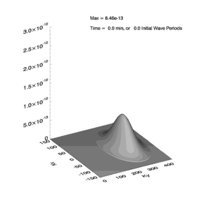
Figure 1: Initial distribution of $|a_{\vec{k}}|^{2}$ on $\vec{k}$-plane.

The simulation was performed until $t=1225$, which is equivalent to $3378\,T_{0}$, where $T_{0}=2\pi/\sqrt{k_{0}}$ is the period of the wave, corresponding to the maximum of the initial spectral distribution.

3.2 Zakharov-Filonenko spectra

Like in the previous papers [10],[12],[13] and [15], we observed fast formation of the spectral tail, described by Zakharov-Filonenko law for the direct cascade $n_{k}\sim k^{-4}$ [5] (see Fig.2). In the agreement with [15], the spectral maximum slowly down-shifts to the large scales region, which corresponds to the inverse cascade [27],[28].

Figure 2: Angle-averaged spectrum $n_{k}=<|a_{\vec{k}}|^{2}>$ in a double logarithmic scale. The tail of distribution fits to Zakharov-Filonenko spectrum.

Also, the direct measurement of energy spectrum has been performed during the final stage of the simulation, when the spectral down shift was slow enough. This experiment can be interpreted as the ocean buoy record – the time series of the surface elevations has been recorded at one point of the surface during $T_{buoy}\simeq 300T_{0}$. The Fourier transform of the autocorrelation function

$$E(\omega)=\frac{1}{2\pi}\int\limits_{-T_{buoy}/2}^{T_{buoy}/2}<\eta(t+\tau)\eta(\tau)>e^{i\omega t}\mathrm{d}\tau\mathrm{d}t.$$ (18)

allows to detect the direct cascade spectrum tail proportional to $\omega^{-4}$ (see Fig.3), well known from experimental observations [29],[30],[31].

Figure 3: Energy spectrum in a double logarithmic scale. The tail of distribution fits to asymptotic $\omega^{-4}$.

In this paper we had no intention to improve results of the previous papers. Inertial interval of the angle-averaged spectra ($\omega$-spectrum also is angle-averaged because it depends only on frequency $\omega\sim\sqrt{k}$) is limited due to anisotropy of the integration domain. In this case we have less than one decade interval and we cannot find an exponent of the Kolmogorov tail surely, however this work was already done in several previous articles (see for instance [13]). Here we limit our observations by qualitative correspondance.

3.3 Is the weak-turbulent scenario realized?

Presence of Kolmogorov asymptotic in spectral tails, however, is not enough to validate applicability of the weak-turbulent scenario for description of wave ensemble. We have also be sure that statistical properties of the ensemble correspond to weak-turbulent theory assumptions.

One should stress out that at the beginning of our experiments $|a_{\vec{k}}|^{2}$ is a smooth function of $\vec{k}$. Only the phases of the individual waves are random. As shows numerical simulation, the initial condition (16) (see Fig.1) does not preserve its smoothness – it becomes rough virtually immediately (see Fig.4).

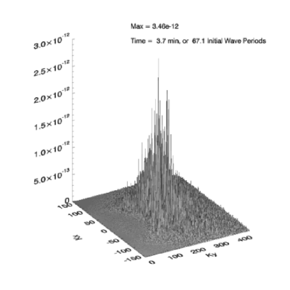
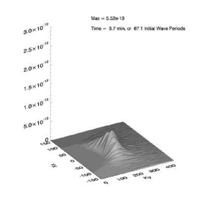
Figure 4: Surface $|a_{\vec{k}}|^{2}$ before (left) and after (right) low-pass filter at the moment of time $t\simeq 67T_{0}$.

The picture of this roughness is remarkably preserved in many details, even as the spectrum down-shifts as a whole. This roughness does not contradict the weak-turbulent theory. According to this theory, the wave ensemble is almost Gaussian, and both real and imaginary parts of each separate harmonics are not-correlated. However, also according to the weak-turbulent theory, the spectra must become smooth after averaging over long enough time of more than $1/\mu^{2}$ periods. Earlier we observed such restoration of the smoothness in the numerical experiments of the $MMT$ model (see [47],[48], [49] and [50]). However, in the experiments discussed in the article, the roughness still persists and the averaging does not suppresses it completely. It can be explained by sparsity of the resonances.

Resonant conditions are defined by the system of equations:

$$\begin{array}[]{c}\displaystyle\omega_{k}+\omega_{k_{1}}=\omega_{k_{2}}+\omega_{k_{3}},\\ \displaystyle\vec{k}+\vec{k}_{1}=\vec{k}_{2}+\vec{k}_{3},\end{array}$$ (19)

These resonant conditions define five-dimensional hyper-surface in six-dimensional space $\vec{k},\vec{k}_{1},\vec{k}_{2}$. In a finite system, (19) turns into Diophantine equation. Some solutions of this equation are known [32], [17]. In reality, however, the energy transport is realized not by exact, but approximate resonances, posed in a layer near the resonant surface and defined by

$$|\omega_{k}+\omega_{k_{1}}-\omega_{k_{2}}-\omega_{k+k_{1}-k_{2}}|\leq\Gamma,$$ (20)

where $\Gamma$ is a characteristic inverse time of nonlinear interaction.

In the finite systems $\vec{k},\vec{k}_{1},\vec{k}_{2}$ take values on the nodes of the discrete grid. The weak turbulent approach is valid, if the density of discrete approximate resonances inside the layer (20) is high enough. In our case the lattice constant is $\Delta k=1$, and typical relative deviation from the resonance surface

$$\frac{\Delta\omega}{\omega}\simeq\frac{\omega_{k}^{\prime}}{\omega}\Delta k=\frac{\omega_{k}^{\prime}}{\omega}\simeq\frac{1}{600}\simeq 2\times 10^{-3}.$$ (21)

Inverse time of the interaction $\Gamma$ can be estimated from our numerical experiments: wave amplitudes change essentially during 30 periods, and one can assume: $\Gamma/\omega\simeq 10^{-2}\gg\frac{\delta\omega}{\omega}$. It means that the condition for the applicability of weak turbulent theory is typically satisfied, but the reserve for their validity is rather modest. As a result, some particular harmonics, posed in certain “privileged” point of $k$-plane could form a network of almost resonant quadruplets and realize significant part of energy transport. Amplitudes of these harmonics exceed the average level essentially. This effect was described in the article [15], where such “selected few” harmonics were called “oligarchs”. If oligarchs realize most part of the energy flux, the turbulence is mesoscopic, not weak.

3.4 Statistics of the harmonics

According to the weak-turbulent scenario, statistics of the $a_{\vec{k}}(t)$ in any given $\vec{k}$ should be close to Gaussian. It presumes that the $PDF$ for the squared amplitudes is

$$P(|a_{\vec{k}}|^{2})\simeq\frac{1}{D}e^{-|a_{\vec{k}}|^{2}/D},$$ (22)

where $D=<|a_{\vec{k}}|^{2}>$ is the mean square amplitude.

To check the equation (22), we need to find the way for calculation of $D(\vec{k})$. If the ensemble is stationary in time, $D(\vec{k})$ could be found for any given $\vec{k}$ by the time averaging. In our case, the process is non-stationary, and we have a problem with determination of $D(\vec{k})$.

To resolve this problem, we used low-pass filtering instead of time averaging. The low-pass filter was taken in the form

$$\begin{array}[]{l}\displaystyle f(\vec{n})=e^{-(|\vec{n}|/\Delta)^{3}},\\ \Delta=0.25\cdot N_{x}/2,\,\,N_{x}=4096.\end{array}$$ (23)

where $\vec{n}$ is integer vector running $K$-space.

This choice of the low-pass filter preserves the values of total energy, wave action and the total momentum within three percent accuracy. The shape of low-pass filtered function is presented on Fig.4.

Now it is possible to average the $PDF$ over different areas in $k$-space. The results for two different moments of time $t\simeq 67.1T_{0}$ and $t\simeq 925T_{0}$ are presented in Fig.5 and Fig.6.

Figure 5: Probability distribution function for relative squared amplitudes $|a_{k}|^{2}/<|a_{k}|^{2}>$. $t\simeq 67T_{0}$. Thin and bold lines – averaging over dissipation and dissipation-free regions of $\vec{K}$-space correspondingly.

Figure 6: Probability distribution function for relative squared amplitudes $|a_{k}|^{2}/<|a_{k}|^{2}>$. $t\simeq 925T_{0}$. Thin and bold lines – averaging over dissipation and dissipation-free regions of $\vec{K}$-space correspondingly.

The thin line gives $PDF$ after averaging over dissipation region harmonics, while bold line presents averaging over the non-dissipative area $|\vec{k}|<k_{d}=1024$. One can see that statistics in the last case is quite close to the Gaussian, while in the dissipation region it deviates from Gaussian distribution. However, deviation from the Guassianity in the dissipation region does not create any problems, since the “dissipative” harmonics do not contain any essential amount of the total energy, wave action and momentum.

One should remember, that the bold lines in the Fig.5 and Fig.6 are the results of averaging over a million of harmonics. Among them there is a population of “selected few”, or “oligarchs”, with the amplitudes exceeding the average value by the factor of more than ten times. The oligarchs exist because our grid is still not fine enough. The contribution of such oligarchs in our case to the total wave action does not exceed 4%. Fifteen leading oligarchs at some moment of time are presented in the Appendix A.

3.5 Two-stage evolution of the swell

Fig. 7-10 demonstrate time evolution of main characteristics of the wave field: wave action, energy, characteristic slope and mean frequency.

Figure 7: Total wave action as a function of time. Solid line — dynamical equations, dashed-dotted line — kinetic equation with artificial viscosity, dashed line — kinetic equation with WAM3 damping term, dotted line — kinetic equation with WAM4 damping term

Figure 8: Total wave energy as a function of time. Solid line — dynamical equations, dashed-dotted line — kinetic equation with artificial viscosity, dashed line — kinetic equation with WAM3 damping term, dotted line — kinetic equation with WAM4 damping term

Figure 9: Average wave slope as a function of time. Solid line — dynamical equations, dashed-dotted line — kinetic equation with artificial viscosity, dashed line — kinetic equation with WAM3 damping term, dotted line — kinetic equation with WAM4 damping term

Figure 10: Mean wave frequency as a function of time. Solid line — dynamical equations, dashed-dotted line — kinetic equation with artificial viscosity, dashed line — kinetic equation with WAM3 damping term, dotted line — kinetic equation with WAM4 damping term

Fig.9 should be specially commented. Here and further we define the characteristic slope as defined in Eq. 11. According to this definition of steepness for the classical Pierson-Moscowitz spectrum $\mu=0.095$. Our initial steepness $\mu\simeq 0.15$ exceeds this value essentially.

Observed evolution of the spectrum can be conventionally separated in two phases. On the first stage we observe fast drop of wave action, slope and especially energy. Then the drop is stabilized, and we observe slow down-shift of mean frequency together with angular spreading. Level lines of smoothed spectra in the first and in the last moments of time are shown in Fig.11-12

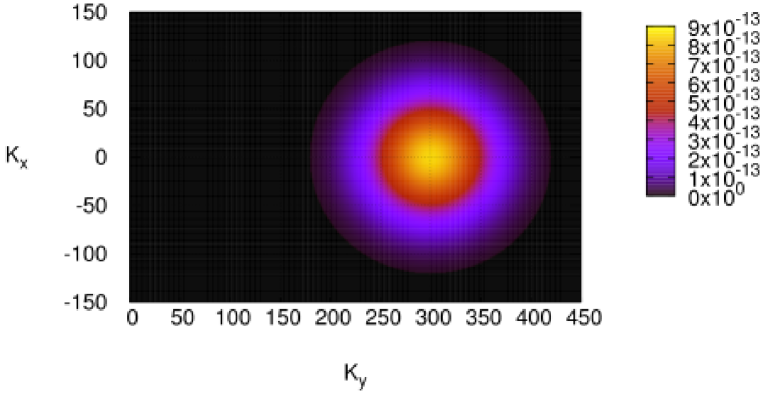
Figure 11: Initial spectrum $|a_{\vec{k}}|^{2}$. $t=0$.

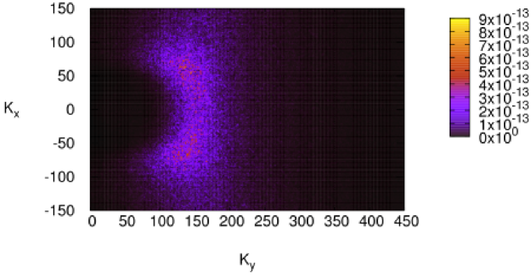
Figure 12: Final spectrum $|a_{\vec{k}}|^{2}$. $t=3378T_{0}$.

Presence of two stages can be understood through the study of the Probability Distribution Functions (PDFs) of the elevations of the surface. In all figures we compare the distribution in experimental results with Gaussian distribution and Tayfun distribution [33]. The later case is just a first correction to Gaussian distribution due to small nonlinearity. We used explicit form of Tayfun distribution following [16]. In the initial moment of time the PDF is Gaussian (see Fig.13). No nonlinear interaction is involved, so Tayfun distribution does not fit at all. However, very soon intensive super-Gaussian tails appear (see Fig.14). They are well described by Tayfun distribution. Then tails decrease slowly (Fig.15), and in the last moment of simulation, when characteristics of the sea are close to Peirson-Moscowitz, the statistics is close to Gaussian again (Fig.16). Moderate tails do exist and, in a good agreement with Tayfun correction, troughs are more probable than crests which in turn can be much larger in absolute value.

Figure 13: PDF for the surface elevation $\eta$ at the initial moment of time. $t=0$.

Figure 14: PDF for the surface elevation $\eta$ at the moment of maximum surface roughness. $t\simeq 14T_{0}$.

Figure 15: PDF for the surface elevation $\eta$ at some middle moment of time. $t\simeq 67.1T_{0}$.

Figure 16: PDF for the surface elevation $\eta$ at the final moment of time. $t=3378T_{0}$.

PDF for $\eta_{y}$ — longitudinal gradients in the first moments of time is Gaussian (Fig.17). Then in a very short period of time strong non-Gaussian tails appear and reach their maximum at $t\simeq 14T_{0}$ (Fig.18). Here $T_{0}=2\pi/\sqrt{k_{0}}$ — period of initial leading wave. Since this moment the non-Gaussian tails decrease. In the last moment of simulation they are essentially reduced(Fig.19).

Figure 17: PDF for $(\nabla\eta)_{y}$ at the initial moment of time. $t=0$.

Figure 18: PDF for $(\nabla\eta)_{y}$ at the moment of maximum surface roughness. $t\simeq 14T_{0}$.

Figure 19: PDF for $(\nabla\eta)_{y}$ at the final moment of time. $t=3378T_{0}$.

Fast growth of non-Gaussian tails can be explained by formation of coherent harmonics. Indeed, $14T_{0}\simeq 2\pi/(\omega_{0}\mu)$ is a characteristic time of nonlinear processes due to quadratic nonlinearity. Note that the fourth harmonic in our system is strongly decaying, hence we cannot see real white caps.

Figures 20-22 present PDFs for gradients in the orthogonal direction.

Figure 20: PDF for $(\nabla\eta)_{x}$ at the initial moment of time. $t=0$.

Figure 21: PDF for $(\nabla\eta)_{x}$ at the moment of maximum surface roughness. $t\simeq 14T_{0}$.

Figure 22: PDF for $(\nabla\eta)_{x}$ at the final moment of time. $t=3378T_{0}$.

Figures 23,24 present snapshots of the surface in the initial and final moments of simulation. Fig.25 is a snapshot of the surface in the moment of maximal roughness $T=4.94\simeq 14T_{0}$.

Figure 23: Surface elevation at the initial moment of time. $t=0$.

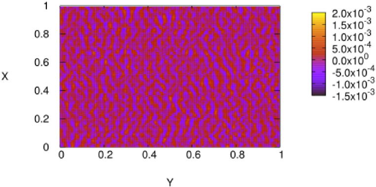
Figure 24: Surface elevation at the final moment of time. $t=3378T_{0}$.

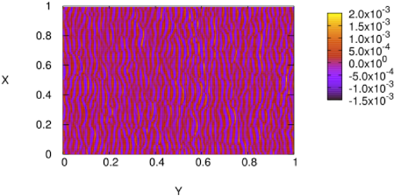
Figure 25: Surface elevation at the moment of maximum surface roughness. $t\simeq 14T_{0}$. Gradients are more conspicuous.

4 Statistical numerical experiment

4.1 Numerical model for Hasselmann Equation

Numerical integration of kinetic equation for gravity waves on deep water (Hasselmann equation) was the subject of considerable efforts for last three decades. The “ultimate goal” of the effort – creation of the operational wave model for wave forecast based on direct solution of the Hasselmann equation – happened to be an extremely difficult computational problem due to mathematical complexity of the $S_{nl}$ term, which requires calculation of a three-dimensional integral at every moment of time.

Historically, numerical methods of integration of kinetic equation for gravity waves exist in two “flavors”.

The first one is associated with works [34], [35], [36], [37], [38] and [39], and is based on transformation of 6-fold into 3-fold integrals using $\delta$-functions. Such transformation leads to appearance of integrable singularities, which creates additional difficulties in calculations of the $S_{nl}$ term.

The second type of models has been developed in works of [40] and [41], [42] and is currently known as Resio-Tracy model. It uses direct calculation of resonant quadruplet contribution into $S_{nl}$ integral, based on the following property: given two fixed vectors $\vec{k},\vec{k_{1}}$, another two $\vec{k_{2}},\vec{k_{3}}$ are uniquely defined by the point “moving” along the resonant curve – locus.

Numerical simulation in the current work was performed with the help of modified version of the second type algorithm. Calculations were made on the grid $71\times 36$ points in the frequency-angle domain $[\omega,\theta]$ with exponential distribution of points in the frequency domain and uniform distribution of points in the angle direction.

To date, Resio-Tracy model suffered rigorous testing and is currently used with high degree of trustworthiness: it was tested with respect to motion integrals conservation in the “clean” tests, wave action conservation in wave spectrum down-shift, realization of self – similar solution in “pure swell” and “wind forced” regimes (see [44], [43], [45]).

Description of scaling procedure from dynamical equations to Hasselman kinetic equation variables is presented in Appendix B.

4.2 Statistical model setup

The numerical model used for solution of the Hasselmann equation has been supplied with the damping term in three different forms:

1. Pseudo-viscous high frequency damping (17) used in dynamical equations;

2. WAM3 viscous term;

3. WAM4 viscous term;

Two last viscous terms are the “white-capping” terms, describing energy dissipation by surface waves due to white-capping, as used in $WAM$ wave forecasting models (in $SWAN$ model the used term has different but close tunable parameters), see [46]:

$$\gamma_{\vec{k}}=C_{ds}\tilde{\omega}\frac{k}{\tilde{k}}\left((1-\delta)+\delta\frac{k}{\tilde{k}}\right)\left(\frac{\tilde{S}}{\tilde{S}_{pm}}\right)^{p}$$ (24)

where $k$ and $\omega$ are wave number and frequency, tilde denotes mean value; $C_{ds}$, $\delta$ and $p$ are tunable coefficients; $S=\tilde{k}\sqrt{H}$ is the overall steepness; $\tilde{S}_{PM}=(3.02\times 10^{-3})^{1/2}$ is the value of $\tilde{S}$ for the Pierson-Moscowitz spectrum (note that the characteristic steepness $\mu=\sqrt{2}S$). It is worth to note that according to [51] theoretical value of steepness for Pierson-Moscovitz spectrum is $S_{PM}\simeq(4.57\times 10^{-3})^{1.2}$. It gives us $\mu\simeq 0.095$.

Values of tunable coefficients for WAM3 case are:

$$C_{ds}=2.36\times 10^{-5},\,\,\,\delta=0,\,\,\,p=4$$ (25)

and for WAM4 case are:

$$C_{ds}=4.10\times 10^{-5},\,\,\,\delta=0.5,\,\,\,p=4$$ (26)

In all three cases we used as initial data smoothed (filtered) spectra (see Fig.4) obtained in the dynamical run at the time $T_{*}=3.65min=24.3\simeq 67.1T_{0}$, which can be considered as a moment of the end of the first “fast” stage of spectral evolution.

The natural question stemming in this point, is why calculation of the dynamical and Hasselmann model cannot be started from the initial conditions (16) simultaneously?

There are good reasons for that:

As it was mentioned before, the time evolution of the initial conditions (16) in presence of the damping term can be separated in two stages: relatively fast total energy drop in the beginning of the evolution and succeeding relatively slow total energy decrease as a function of time, see Fig.8. We explain this phenomenon by existence of the effective channel of the energy dissipation due to strong nonlinear effects, which can be associated with the white-capping as we mentioned in the introduction.

We have started with relatively steep waves $\mu\simeq 0.167$. As we see, at that steepness white-capping is the leading effect. This fact is confirmed by numerous field and laboratory experiments. From the mathematical view-point, the white-capping is formation of coherent structures – strongly correlated multiple harmonics. The spectral peak is posed in our experiments initially at $k\simeq 300$, while the edge of the damping area $k_{d}\simeq 1024$. Hence, only the second and the third harmonic can be developed, while higher harmonics are suppressed by strong dissipation. Anyway, even formation of the second and the third harmonic is enough to create intensive non-Gaussian tail of the $PDF$ for longitudinal gradients. This process is very fast. In the moment of time $T=14T_{0}$ we see fully developed tails. Relatively sharp gradients mimic formation of white caps. Certainly, the “pure” Hasselmann equation is not applicable on this early stage of spectral evolution, when energy intensively dissipates.

As steepness decreases and spectral maximum of the swell down-shifts, the efficiency of such mechanism of energy absorption becomes less important. When the steepness value drops down to $\mu\simeq 0.1$, at approximately $T\simeq 280T_{0}$, the white-capping is negligibly small. Therefore, we decided to start comparison between deterministic and statistical modeling in some intermediate moment of time $T\simeq 67.1T_{0}$.

5 Comparison of deterministic and statistical experiments.

5.1 Statistical experiment with pseudo-viscous damping term.

The first series of statistical experiments has been performed with pseudo-viscous damping term (17).

Fig.7 – 10 show total wave action, total energy, mean wave slope and mean wave frequency as the functions of time.

Fig.31 shows the time evolution of angle-averaged wave action spectra as the functions of frequency for dynamical and Hasselmann equations. We see similar down-shift of the spectral maximum both in dynamic and Hasselmann equations. The correspondence of the spectral maxima amplitudes is not good at all.

It is quite obvious that the influence of the artificial viscosity is not strong enough to reach the correspondence of two models.

5.2 Statistical experiments with WAM3 damping term

The second series of statistical experiments has been done for the choice of WAM3 damping term.

The temporal behavior of total wave action, energy and average wave slope (see Fig.7 – 10) for WAM3 damping term is in better correspondence with dynamical model, than in the case of artificial viscosity term. For initial $50\,min$ duration of the experiment we observe decent correspondence between dynamical and Hasselmann equations. For longer time the WAM3 model, however, deviates from the dynamical model significantly.

As in the artificial viscosity case, the angle-averaged wave action spectra as the function of frequency exhibit distinct down-shift of the spectral maxima for both dynamical and Hasselmann equations (see Fig.32). Correspondence between time evolution of the amplitudes of the spectral maxima is also much better for WAM3 choice of damping, than for artificial viscosity case.

Presumably, WAM3 damping term underestimate the effects of real damping at the very beginning of the evolution (when the effects of white capping are relatively important), and overestimates them on later stages of swell evolution.

5.3 Statistical experiments with WAM4 damping term

The final third series of experiments have been done for the choice of WAM4 damping term.

Fig.7–10 show temporal evolution of the total wave action, total energy, mean wave slope and mean wave frequency, which are divergent in time in this case.

Fig.33 show time evolution of angle-averaged wave action spectra as the functions of frequency for dynamical and Hasselmann equations. While as in the artificial viscosity and WAM3 cases we also observe distinct down-shift of the spectral maxima, the correspondence of the time evolution of the amplitudes of the spectral maxima is worse than in WAM3 case.

This observation is especially surprising in view of the fact that historically WAM4 damping has been invented as an improvement to WAM3 damping term. It is quite obvious that WAM4 damping is too strong for description of the reality at all stages of the swell evolution.

6 Down-shift and angular spreading

The major process of time-evolution of the swell is frequency down-shift. During $T=933T_{0}$ the mean frequency has been decreased from $\omega_{0}=2$ to $\omega_{1}=0.6$. On the last stage of the process, the mean frequency slowly decays as

$$<\omega>\sim t^{-0.067}\simeq t^{-1/15}$$ (27)

The Hasselmann equation has self-similar solution, describing the evolution of the swell $n(\vec{k},t)\sim t^{4/11}F\left(\frac{\vec{k}}{t^{2/11}}\right)$ (see [43], [45]). For this solution

$$<\omega>\sim t^{-1/11}$$ (28)

The difference between (27) and (28) can be explained as follows. What we observed, is not a self-similar behavior. Indeed, a self-similarity presumes that the angular structure of the solution is constant in time. Meanwhile, we observed intensive angular spreading of the initially narrow in angle, almost one-dimensional wave spectrum.

Level lines of the low-pass filtered dynamic and kinetic spectrum at the beginning of the simulation are presented on Fig.26-26. There are ten isolines on every figure. Values of level at maximum and minimum isolines are shown on every picture.

Figure 26: Level lines of the dynamic (left) and the kinetic (right) spectra at $t=67.1\,T_{0}$.

Level lines of the low-pass filtered dynamic and kinetic spectrum for three different damping terms at the end of the simulation are presented on Fig.27-28.

Figure 27: Level lines of the dynamic (left) and the kinetic (right) spectra at $t=3378.2\,T_{0}$.

Figure 28: (left)Level lines of the kinetic spectra in the WAM3 (left) WAM4 and damping cases at $t=3378.2\,T_{0}$.

We observed development of bimodality in both experiments. This is in accordance with field observations [53], [54].

One can see good correspondence between the results of both experiments. Comparison of time-evolution of the mean angular spreading, calculated from action and energy spectra is presented on Fig. 29-30.

Figure 29: Average angular spreading $\left(\int|\theta|n(\vec{k})\mathrm{d}\vec{k}\right)/\left(\int n(\vec{k})\mathrm{d}\vec{k}\right)$ as a function of time, calculated from wave action. Solid line - WAM3, dotted line - WAM4, dashed line - artificial viscosity, stars - dynamical equations

Figure 30: Average angular spreading $\left(\int|\theta|\omega n(\vec{k})\mathrm{d}\vec{k}\right)/\left(\int\omega n(\vec{k})\mathrm{d}\vec{k}\right)$ as a function of time, calculated from wave energy. Solid line - WAM3, dotted line - WAM4, dashed line - artificial viscosity, stars - dynamical equations

We see growing divergence between dynamic and kinetic models. But using WAM3 and WAM4 models leads to worse divergence. This is an additional argument against these variants of white-cap damping.

One can expect that the angular spreading will be arrested at later times, and the spectra will take universal self-similar shape.

Figure 31: Angle-averaged spectrum as a function of time for dynamical and Hasselmann equations for artificial viscosity case.

Figure 32: Angle-averaged spectrum as a function of time for dynamical and Hasselmann equations a function of time for WAM3 case.

Figure 33: Angle-averaged spectrum as a function of time for dynamical and Hasselmann equations a function of time for WAM4 case.

7 Conclusion

1. Our numerical experiment shows that the Hasselmann equation without any additional terms is applicable for description of gravity waves turbulence in the infinite basin only if nonlinearity is low enough. The average wave steepness $\mu=({E^{2}}/{N^{2}})sqrt{2E}$ should be significantly less a certain critical level $\mu_{0}=0.095$. To describe the wave turbulence of a moderate steepness $0.095<\mu<0.15$, one should add to the Hasselmann equation some additional term $S_{diss}$ modeling dissipation due to white-capping. So far there is no any theory making possible to find $S_{diss}$ analytically. This is a great challenge for hydrodynamicists. So far we can suggest that $S_{diss}$ depends on steepness very sharply. Hence the guess that white-capping is the threshold phenomenon formulated by Banner, Babanin, and Young [52] looks very plausible. We did not model too steep waves, but we can conjecture that if $\mu>0.15$, white capping is the leading nonlinear process and the weak-turbulent approach is not applicable at al.

2. Our results are not a surprise for designers of operational models for wave forecasting. They understood necessity to introduce into the models extra dissipative terms many years ago. Another story that the models of $S_{diss}$ routinely used in the WAM and WAVEWATCH models are too crude and do not grasp the most important feature of the white-capping — its threshold nature. In our opinion existing models of $S_{diss}$ overestimate dissipation at small values of steepness and underestimate it at large $\mu$. Moreover, they overestimate dissipation in the area of the spectral peak and underestimate it in the spectral region of high wave numbers. We are planning to offer our own form of $S_{diss}$ extracted from our massive numerical simulation of Euler equation, but it will take some time and toil.

3. We have to stress that we solved maximally idealized model. We did not take into account interaction of swell with atmosphere (see for instance [55], [56] ), interaction with ocean currents, deviation of the wave motion from potentiality as well as influence of turbulence in the surface-atmosphere boundary layer. In the future we plan to establish a contact with experimentalists to develop more realistic model of swell propagation in the real ocean.

4. In one aspect our conclusions are very resolute. All existing experimental wave tanks cannot be used for modelling of the waves propagation in open sea. The mesoscopic effects in wave tanks are too strong for reasonable values of steepness. This pertains only to modeling of kinetics of energy containing region in the vicinity of spectral peak. The rear faces of spectral distributions, spectral tails, can be successfully modelled. This was demonstrated by Toba in his classical work [29]. Toba observed the Zakharov-Filonenko spectrum $I_{\omega}\sim\omega^{-4}$ in the wave tank of moderate size. In our opinion this conclusion is very important. Some authors, trying to find the universal law of fetch dependence of mean energy and mean frequency put together data collected in ocean and in the experimental tanks. This mixed data hardly can be compared with any self sufficient theory. This question is discussed in details in the article [57].

Another conclusion is more pessimistic. The results of numerical experiments show that it is very difficult to reproduce real ocean conditions in laboratory wave tank. Even the size of the tanks of $200\times 200$ meters is not large enough to model ocean due to the presence of wave numbers grid discreteness.

8 Acknowledgments

This work was supported by ONR grant N00014-06-C-0130, US Army Corps of Engineers Grant W912HZ-04-P-0172, RFBR grant 06-01-00665-a, INTAS grant 00-292, the Programme “Nonlinear dynamics and solitons” from the RAS Presidium and “Leading Scientific Schools of Russia” grant, also by and by NSF Grant NDMS0072803. We use this opportunity to greatfully acknowledge the support of these foundations.

A. O. Korotkevich was also supported by Russian President grant for young scientist MK-1055.2005.2.

Also authors want to thank the creators of the open-source fast Fourier transform library FFTW [58] for this fast, portable and completely free piece of software.

Appendix A “Forbes” list of 15 largest harmonics.

Here one can find 15 largest harmonics at the end of calculations in the framework of dynamical equations. Average square of amplitudes in dissipation-less region was taken from smoothed spectrum, while all these harmonics exceed level $|a_{\vec{k}}|^{2}=1.4\times 10^{-12}$. $K_{x}$ $K_{y}$ $|a_{\vec{k}}|^{2}$ $<|a_{\vec{k}}|^{2}>_{f}$ $\frac{|a_{\vec{k}}|^{2}}{<|a_{\vec{k}}|^{2}>}$ -59 155 1.563e-12 0.746e-13 2.095e+1 -37 166 1.903e-12 1.201e-13 1.585e+1 -37 185 1.569e-12 2.288e-13 0.686e+1 -36 162 1.477e-12 0.992e-13 1.489e+1 -33 157 1.442e-12 0.713e-13 2.022e+1 -26 164 3.351e-12 0.847e-13 3.956e+1 -17 189 1.463e-12 2.789e-13 0.525e+1 -14 173 1.408e-12 1.459e-13 0.965e+1 -2 176 1.533e-12 1.697e-13 0.903e+1 0 177 2.066e-12 1.741e-13 1.187e+1 10 179 1.427e-12 1.893e-13 0.754e+1 27 163 1.483e-12 0.832e-13 1.782e+1 31 174 1.431e-12 1.342e-13 1.066e+1 37 173 1.578e-12 1.581e-13 0.998e+1 60 133 1.565e-12 0.345e-13 4.536e+1

Appendix B From Dynamical Equations to Hasselmann Equation.

Standard setup for numerical simulation of the dynamical equations (4) implies $2\pi\times 2\pi$ domain in real space and gravity acceleration $g=1$. Usage of the domain size equal $2\pi$ is convenient because in this case wave numbers are integers.

In the contrary to dynamical equations, the kinetic equation (12) is formulated in terms of real physical variables and it is necessary to describe the transformation from the “dynamical” variables into to the “physical” ones.

Eq.4 are invariant with respect to “stretching” transformation from “dynamical” to “real” variables:

$$\eta_{\vec{r}} = \alpha\eta_{\vec{r}^{\prime}}^{\prime},\,\,\,\,\vec{k}=\frac{1}{\alpha}\vec{k}^{\prime},\,\,\,\,\vec{r}=\alpha\vec{r}^{\prime},\,\,\,\,g=\nu g^{\prime},$$ (29)

$$t = \sqrt{\frac{\alpha}{\nu}}t^{\prime},\,\,\,L_{x}=\alpha L_{x}^{\prime},\,\,\,L_{y}=\alpha L_{y}^{\prime}$$ (30)

where prime denotes variables corresponding to dynamical equations.

In current simulation we used the stretching coefficient $\alpha=800.00$, which allows to reformulate the statement of the problem in terms of real physics: we considered $5026\,m\times 5026\,m$ periodic boundary conditions domain of statistically uniform ocean with the same resolution in both directions and characteristic wave length of the initial condition around $22\,m$. In oceanographic terms, this statement corresponds to the “duration-limited experiment”.

References

- [1] L.W. Nordheim, Proc.R.Soc., A 119, 689 (1928).
- [2] R. Peierls, Ann. Phys. (Leipzig), 3, 1055 (1929).
- [3] V. E. Zakharov, G. Falkovich, and V. S. Lvov, Kolmogorov Spectra of Turbulence I (Springer-Verlag, Berlin, 1992).
- [4] K. Hasselmann, J.Fluid Mech., 12, 48, 1 (1962).
- [5] V. E. Zakharov and N. N. Filonenko, Doklady Acad. Nauk SSSR, 160, 1292 (1966).
- [6] A. N. Pushkarev and V. E. Zakharov, Phys. Rev. Lett. 76, 18, 3320 (1996).
- [7] A. N. Pushkarev, European Journ. of Mech. B/Fluids 18, 3, 345 (1999).
- [8] A. N. Pushkarev and V. E. Zakharov, Physica D 135, 98 (2000)
- [9] M. Tanaka, Journ. Fluid Mech. 444, 199 (2001).
- [10] M. Onorato, A. R. Osborne, M. Serio at al., Phys. Rev. Lett. 89, 14, 144501 (2002). arXiv:nlin.CD/0201017
- [11] K. B. Dysthe, K. Trulsen, H. E. Krogstad and H. Socquet-Juglard, J. Fluid Mech. 478, 1-10 (2003).
- [12] A. I. Dyachenko, A. O. Korotkevich and V. E. Zakharov, JETP Lett. 77, 10, 546 (2003). arXiv:physics/0308101
- [13] A. I. Dyachenko, A. O. Korotkevich and V. E. Zakharov, Phys. Rev. Lett. 92, 13, 134501 (2004). arXiv:physics/0308099.
- [14] N. Yokoyama, J. Fluid Mech. 501, 169 (2004).
- [15] V. E. Zakharov, A. O. Korotkevich, A. N. Pushkarev and A. I. Dyachenko, JETP Lett. 82, 8, 487 (2005). arXiv:physics/0508155.
- [16] H. Socquet-Juglard, K. Dysthe, K. Trulsen, H. E. Krogstad, and J. Liu, J. Fluid Mech., 542, 195 (2005).
- [17] Yu. Lvov, S. V. Nazarenko and B. Pokorni, Physica D 218, 1, 24 (2006). arXiv:math-ph/0507054.
- [18] S. V. Nazarenko, J. Stat. Mech. L02002 (2006). arXiv:nlin.CD/0510054.
- [19] A. I. Dyachenko, F. Dias and V. E. Zakharov, in preparation (2007).
- [20] S. Yu. Annenkov and V. I. Shrira, Phys. Rev. Lett. 96, 204501 (2006).
- [21] A. I. Dyachenko, A C. Newell, A. Pushkarev and V. E. Zakharov, Physica D 57, 96 (1992).
- [22] A. O. Korotkevich, PhD thesis, L.D. Landau Institute for Theoretical Physics RAS, Moscow, Russia (2003).
- [23] A. I. Dyachenko, A. O. Korotkevich and V. E. Zakharov, JETP Lett. 77, 9, 477 (2003). arXiv:physics/0308100
- [24] V. E. Zakharov, J. Appl. Mech. Tech. Phys. 2, 190 (1968).
- [25] V. E. Zakharov, Eur. J. Mech. B/Fluids, 18, 327 (1999).
- [26] A. Kolmogorov, Dokl. Akad. Nauk SSSR 30, 9 (1941) [Proc. R. Soc. London A434, 9 (1991)].
- [27] V. E. Zakharov, PhD thesis, Budker Institute for Nuclear Physics, Novosibirsk, USSR (1967).
- [28] V. E. Zakharov and M. M. Zaslavskii, Izv. Atm. Ocean. Phys. 18, 747 (1982).
- [29] Y. Toba, J. Oceanogr. Soc. Jpn. 29, 209 (1973).
- [30] M. A. Donelan, J. Hamilton and W. H. Hui, Phil. Trans. R. Soc. London, A315, 509 (1985)
- [31] P. A. Hwang at al., J. Phys. Oceanogr. 30, 2753 (2000).
- [32] A. I. Dyachenko and V. E. Zakharov, Phys. Lett., A 190, 144 (1994).
- [33] A. Tayfun, Journ. of Geophys. Res., 85, 1548 (1980).
- [34] S. Hasselmann, K. Hasselmann, T. P. Barnett, J. Phys. Oceanogr., 15, 1378 (1985).
- [35] J. C. Dungey, W. H. Hui, Proc. R. Soc., A368, 239 (1985).
- [36] A. Masuda, J. Phys. Oceanogr., 10, 2082 (1981).
- [37] A. Masuda in: O. M. Phillips, K. Hasselmann, Waves Dynamics and Radio Probing of the Ocean Surface, Plenum Press, New York (1986).
- [38] I. V. Lavrenov, Mathematical modeling of wind waves at non-uniform ocean, Gidrometeoizdat, St.Petersburg, Russia (1998).
- [39] V. G. Polnikov, Wave Motion, 1008, 1 (2001).
- [40] D. J. Webb, Deep-Sea Res., 25, 279 (1978).
- [41] D. Resio, B. Tracy, Theory and calculation of the nonlinear energy transfer between sea waves in deep water, Hydraulics Laboratory, US Army Engineer Waterways Experiment Station, WIS Report 11 (1982).
- [42] D. Resio, W. Perrie, J.Fluid Mech., 223, 603 (1991).
- [43] A. Pushkarev, D. Resio, V. E. Zakharov, Physica D, 184, 29 (2003).
- [44] A. Pushkarev, V. E. Zakharov,6th International Workshop on Wave Hindcasting and Forecasting, November 6-10, Monterey, California, USA), 456 (published by Meteorological Service of Canada) (2000).
- [45] S. I. Badulin, A. Pushkarev, D. Resio and V. E. Zakharov, Nonlinear Processes in Geophysics (2005).
- [46] SWAN Cycle III user manual, http://fluidmechanics.tudelft.nl/swan/index.htm
- [47] V. E. Zakharov, P. Guyenne and F. Dias, Physica D, 152-153, 573 (2001).
- [48] F. Dias, A. Pushkarev and V. E. Zakharov, Physics Reports, 398, 1 (2004).
- [49] F. Dias, P. Guyenne, A. Pushkarev, V. E. Zakharov, Preprint N2000-4, Centre de Methematiques et del leur Appl., E.N.S de CACHAN, 1 (2000).
- [50] P. Guyenne, V. E. Zakharov, F. Dias Contemporary Mathematics, 283, 107 (2001).
- [51] I. R. Young, Wind generated ocean waves, (Elsevier, Amsterdam, the Netherlands, 1999).
- [52] M. L. Banner, A. V. Babanin, and I. R. Young, Journ. Phys. Oceanogr., 30, 12, 3145 (2000).
- [53] K. C. Ewans, Journ. Phys. Oceanogr., 28, 3, 195 (1998).
- [54] D. W. Wang and P. A. Hwang, Journ. Phys. Oceanogr., 31, 5, 1200 (2001).
- [55] W. M. Drennan, H. C. Graber, and M. A. Donelan, Journ. Phys. Oceanogr., 29, 8, 1853 (1999).
- [56] A. A. Grachev, C. W. Fairall, J. E. Hare, J. B. Edsond, and S. D. Miller, Journ. Phys. Oceanogr., 33, 11, 2408 (2003).
- [57] S. I. Badulin, A. V. Babanin, V. E. Zakharov, and D. Resion, submitted in Journ. Fluid Mech. (2007).
-
[58]
http://fftw.org
M. Frigo and S. G. Johnson, Proc. IEEE 93, 2, 216 (2005).