Detecting and localizing the foci in human epileptic seizures

Abstract

We consider the electrical signals recorded from a subdural array of electrodes placed on the pial surface of the brain for chronic evaluation of epileptic patients before surgical resection. A simple and computationally fast method to analyze the interictal phase synchrony between such electrodes is introduced and developed with the aim of detecting and localizing the foci of the epileptic seizures. We evaluate the method by comparing the results of surgery to the localization predicted here. We find an indication of good correspondence between the success or failure in the surgery and the agreement between our identification and the regions actually operated on.

Epilepsy is defined as a condition of chronic unprovoked seizures. It is one of the most common neurologic disorders, affecting more than 50 million people worldwide. About 1/3 of cases are not adequately controlled by medication, causing a severe reduction in independence and quality of life. If an individual’s seizures are stereotyped and appear to have a focal onset, surgical resection may be a consideration. Localizing accurately the epileptic focus (or foci) is therefore essential part of surgical planning. We propose a simple and computationally fast method based on phase synchronization, that is able to correctly localize the foci of epileptic seizures. The method was applied to the data of three patients. The overlap of the location of the electrodes identified by our method and the resected areas was consistent with the degree of surgery success.

I Introduction

Epilepsy is defined as a condition of chronic unprovoked seizures. It is one of the most common neurologic disorders, affecting more than 50 million people worldwide. About 1/3 of cases are not adequately controlled by medication, causing a severe reduction in independence and quality of life. Seizures often begin in one brain region and rapidly spread to other areas of cortex, manifesting in a wide variety of symptoms, ranging from a brief staring spell (absence seizures), to generalized convulsions (grand mal seizures). The mechanisms of seizure spread are not yet well understood. If an individual’s seizures are stereotyped and appear to have a focal onset, surgical resection may be a consideration.

As part of the invasive surgical evaluation, arrays of electrodes are chronically implanted onto the surface of the brain (Fig.1) in order to record the onset and evolution of several spontaneous seizures. The ensemble of signals [called the electrocorticogram (ECoG)] is simultaneously recorded and analyzed for detecting the proper cortical area to be resected schiff . Decisions regarding which areas of cortex to resect are made by board-certified epileptologists, based on careful review of the onset and spread of several spontaneous seizures. The goal is to remove the epileptogenic zone, the minimal area of cortex that is necessary and sufficient to prevent further seizures from recurring, if it is not located in eloquent cortical areas that are critical for normal function.

The clinical challenge is how to analyze the ECoG signals to achieve a simple, automatic, data-driven, fast and reliable identification of the epileptic focus. Traditionally, linear measures, such as correlation coefficients, were utilized to complement the visual inspection. In the last two decades methods based on the nonlinear measures were introduced to the field.

It has been shown that a significant reduction of the dimension of the system CorDim ; lehn01 (as measured by the correlation dimension GP and by the neuronal complexity loss) occur in the vicinity of the epileptic focus, not only during the seizures (ictal periods), but also between seizures (inter-ictal periods).

The interdependence between signals from different sites, studied by means of nonlinear cross-predictability and mutual nonlinear predictability Arnold-InderDep ; Queyen-interDep , also allows the location of the focus. Surrogate-corrected nonlinear measures And06 were shown to correctly identify the focal hemisphere in the inter-ictal recordings. Many of these methods involve the reconstruction of the phase space by time-delay embedding embedding . Such measures calculated from noisy non-stationary time series usually can not be directly related to the dimensionality of the attractor stam05 and the calculations are computationally costly.

Recently, concepts from synchronization analysis were brought to the study of ECoG signals stam05 ; stam ; quian ; schindler ; schevon ; bia06 ; palus01 , leading to a series of promising results on localization and predictability of epileptic seizures. In most of these works the increase in the synchronization was found only during the seizure, while synchronization clusters, identified in bia06 , remain synchronized also during inter-ictal periods. Similar stability of local hyper-synchronous regions was found also in schevon . In spite of demonstrated success, formulation of these methods involve some assumptions, that we would like to relax in our proposed approach, as it will be explained in the next Section.

The aim of this paper is twofold. First, we describe a model-free and fast approach, based on phase synchronization, that is able to identify the epileptic focus. Second, we apply the method to ECoG data of three patients, and show that there is a good correspondence between the success or failure in surgery and the overlap between the area spanned by the electrodes identified by our method and that of the brain tissue actually removed.

II Method

II.1 Patients and ECoG recordings

In this paper we analyze the ECoG data from three female patients with intractable partial complex seizures with secondary generalization, referred to as patients A, B and C, respectively.

Patient A is a 17 years old and had her first seizure at age six. Her magnetic resonance imaging (MRI) was normal, but a positron emission tomography (PET) scan revealed reduced metabolism of the left temporal and parietal lobes. Spontaneous seizures originated in the temporal lobe and spread posteriorly. A total of 80 electrodes were implanted in 4 arrays, with 16 eletrodes at the temporal lobe. A left temporal lobectomy was performed, leaving her seizure-free for the last two years (Engel class I, see Ref. engel for the classification of the surgery outcome).

Patient B is a 12 years old with a history of developmental delay and seizures since 8 month of age. Before surgery she experienced as many as 30 seizures/day. Although her MRI was normal, a PET study revealed general hypometabolism of the cerebral cortex. 96 electrodes in 5 arrays were implanted, with 32 electrodes in frontal grid (F), 32 electrodes in parietal grid (P) and 24 electrodes at the temporal lobe in three strips (AT, ST and PT, cf. Fig. 2). She received a left frontal and occipital topectomy. She had an Engel Class III outcome.

Patient C is a 7 years old and the outcome was Engel class II 16 months after operation, while 3 years after surgery she has frequent seizures. She was implanted with 96 electrodes, 64 of which were in the parietal grid, and 32 electrodes at the temporal lobe.

For all patients all subdural electrode channels were referenced to a scalp electrode on the midline (CPz) and then the grand mean was subtracted from each channel to remove the contribution of the reference electrode.

We have analyzed a total of 24 hours of ECoG recordings (mean 8 hours, range 200 minutes-15 hours 30 minutes), containing a total of 12 seizures (mean 4, range 3-5). The data were recorded with a sampling frequency of 400 Hz and band-pass filtered offline to 0.5-50 Hz using moving overlapping windows and a finite impulse response filter with a Kaiser window.

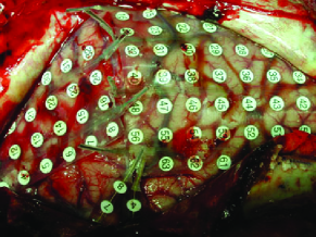
Figure 1: (Color online) Subdural ECoG grid of electrodes placed on the surface of the brain for chronic evaluation of epileptic patients before surgical resection.

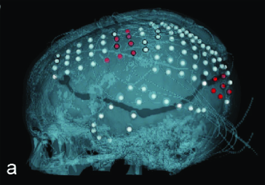
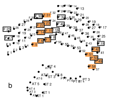
Figure 2: (Color online) The computed tomography (CT) image with marked electrodes (a) and the electrode scheme (b), projected on the plane, for patient B. The arrays of electrodes are labeled according to their position: F- frontal, P- parietal, AT-anterior temporal, ST - sub-temporal, PT - posterior-temporal. The same naming convention is used for all patients. For description of other marks see discussion after Eq. 4.

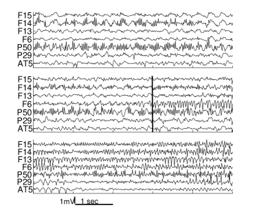
Figure 3: Voltage traces of ECoG signals. Three 10 s portions of voltage traces of 7 electrodes, taken from a multielectrode recording of 96 electrodes of patient B, cf. Fig. 2. The seizure onset is marked by a vertical line. The analysis below indicates that the signals coming from electrodes F6, F14, F15 and P50 belong to the epileptic foci, whereas the F13, P29 and AT5 do not. The voltage scale of 1 mV and the time scale of 1 second are shown below the figure.

II.2 Synchronization Strength Diagrams

To see the main concepts behind the method, consider a one-dimensional oscillatory signal $x(t)$. The associated phase space can be fully reconstructed by using the coordinates $x(t)$, $dx(t)/dt$, $d^{2}x(t)/dt^{2},~{}\dots$, with as many derivatives as needed to exhaust the dimensionality of the system. In such a reconstructed phase space one can then define the Poincaré section by noting the points obtained when the orbit crosses the surface $dx(t)/dt=0$. Obviously, this surface coincides with the points of minima or maxima in the original one-dimensional signal $x(t)$. In this work we focus on the points of maxima, and define the phase $\phi(t)$ of the trajectory by increasing its value by 2$\pi$ after each maximum. Precisely, between the $k$th maximum occurring at $t=t_{k}$ and the $(k+1)$th maximum occurring at $t_{k+1}$, we define the phase over the period of time $t_{k}\leq t\leq t_{k+1}$ using the linear interpolation rose ; bocca02

$$\phi(t)=2\pi k+2\pi\frac{t-t_{k}}{t_{k+1}-t_{k}}\quad(t_{k}<t<t_{k+1})\ .$$ (1)

Note that the resulting monotonically increasing phase does not contain any information about the amplitude of the original signal and thus the results of the analysis are not affected by the amplitude variation sharry .

Phases can be affected by instrumental artifacts; we have carefully ascertained that any signal segments that appear identical in all recording channels were manually excluded from the signal prior to calculation of the phases. It is important to remark that our data feature broad band spectra. Alternative measures of the phase (such as the one based on the Hilbert transform) imply the presence of a prominent spectral peak bocca02 . We would like to avoid any a priori assumptions on the spectral structure of the signals, therefore we opted for the above definition of phase, Eq. 1.

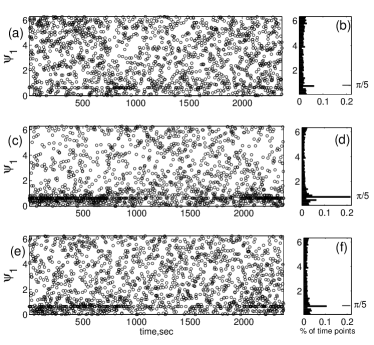
Figure 4: Panels (a),(c) and (e): Synchrograms for 3 neighboring pairs of electrodes along [F13-F14 (a), F15-F14(c)] and across the grid [F6-F14 (e)], calculated for the reference electrode F14 (the signals for F6, F13, F14 and F15 are shown in Fig.3). Since the synchronization line appears at $\psi_{1}=0$, a small phase offset of $\phi_{\rm sh}=\pi/5$ was added to the phase $\phi_{y}$ for clarity. Panels (b),(d), and (f) show the histograms of the phase points distribution within the corresponding synchrogram. Clearly, only one strong line is present in each synchrogram, at the position of the offset phase ($\pi/5$). This corresponds to the 1:1 synchronization without visible phase difference.

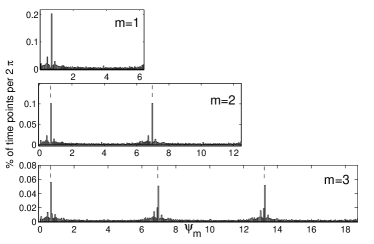
Figure 5: Histograms for synchrograms of orders $m=1,2$ and $3$ calculated for the pair of electrodes F14-F15 (cf. Fig. 4, c and d). The dashed lines mark offset positions $\pi/5,2\pi+\pi/5$ and $4\pi+\pi/5$. The same bin size ( $2\pi/100$) was used in all histograms. The number of strong lines equals to the order of the synchrogram, confirming the 1:1 synchronization. The position of the synchronization lines coincide with the value of the offset phase within $\pm\pi/50$.

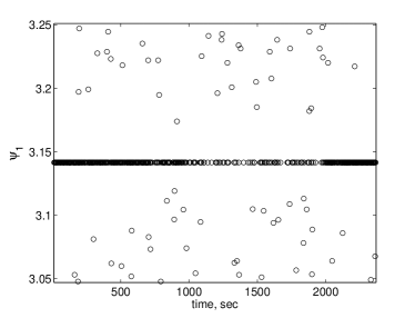
Figure 6: The vicinity of the 1:1 synchronization line for synchrogram of electrodes F14 and F15, with the phase offset $\phi_{\rm sh}=\pi$. Note that the synchronization line is clearly isolated.

The notion of phase synchronization rose ; bocca02 refers to a process wherein a locking of the phases of weakly coupled oscillators is produced, without implying a substantial correlation in the oscillators’ amplitudes. The same concept can be related to our case, for measuring the degree of phase synchronization of two different signals, say $x(t)$ and $y(t)$. Using the basic definition (1), one can indeed produce the phases of each signal, denoted as $\phi_{x}(t)$ and $\phi_{y}(t)$, respectively. Taking $x(t)$ as the reference signal, one can further consider the time points of its maxima $t_{k}$, and read the phase $\phi_{y}(t_{k})$ at these time points. One then defines the following reduced phases $\psi_{m}(t_{k})$ according to

$$\psi(t_{k}) = \phi_{y}(t_{k})~{}{\rm mod}2\pi\ ,$$

$$\psi_{2}(t_{k}) = \phi_{y}(t_{k})~{}{\rm mod}4\pi\ ,$$

$$\dots \ ,$$

$$\psi_{m}(t_{k}) = \phi_{y}(t_{k})~{}{\rm mod}~{}2\pi m\ .$$ (2)

The graphic representation of $\psi_{m}(t_{k})$ vs. $t_{k}$ is called a synchrogram of order $m$. We will consider the signals $x(t)$ and $y(t)$ as synchronized at ratio $n:m$ when the $m$th order synchrogram exhibits $n$ distinct horizontal lines (i.e. fixed reduced phase $\psi_{m}(t_{k})$ for a series of time $t_{k}$). Synchrograms, indeed, have been proved to be useful to visualize and trace transitions between different ratios of phase locking in biological data, as the cardiorespiratory system of a human subject naturekurths , where non-stationarity is often strong. Note that $\psi_{m}(t_{k})$ is, in general, not symmetric, and, within the same pair of signals, may depend on which electrode is taken as a reference bocca02 . An addition of any constant phase $\phi_{\rm sh}$ to $\phi_{y}(t)$ does not change the synchronization ratio, but merely shifts the position of the synchronization lines. Such an offset may facilitate the visualization of the line when it appears close to the edge of the synchrogram.

To exemplify this notion in the present context, we use the data of the patient B. In Fig 2 we show the CT image with the electrode positions marked on it and the plane projection of the electrode placement scheme. In Fig. 3 the three 10 sec portions of signals from seven electrodes are plotted. These portions of the signal correspond to the time near the seizure onset. The signals from five of these electrodes are used in Figs. 4-9.

We present in Fig. 4 synchrograms constructed from the signals associated with three neighboring pairs of electrodes, which display the presence of 1:1 phase synchronization. The fraction of the time, during which the signals are synchronized, differs significantly, albeit the same geometrical distance between these pairs of electrodes.

To test for the presence of more complicated synchronization ratios, we calculated the synchrograms of higher orders. The histograms for them are shown in Fig 5. The number of strong lines in each histogram is equal to the order of the corresponding synchrogram, thus confirming the dominant 1:1 synchronization ratio. Note that this ratio is usually assumed in the methods involving phase difference lehn01 ; schevon ; bia06 . We do not make such an assumption. In fact, any synchronization ratio may be treated on the same footing. In the following analysis we concentrate on the first order synchrograms $\psi_{1}$ with the phase offset $\phi_{\rm sh}=\pi$. The phase points that belong to the synchronization line may be easily extracted from the synchrogram, since they are clearly isolated from other points (see Fig 6).

The present method shares some similarities with the so-called event-synchronization technique quian , though this latter strategy is, in general, unable to distinguish between different types of $n:m$ lockings. The information contained in the synchrograms can be easily employed to extract the level of phase synchronization between all the pairs of electrodes at our disposal. To this aim we define the statistical strength of synchronization $S_{ij}(t)$ (SS) of every given electrode $i$ to any other electrode $j$: we take the synchrogram of electrodes $i$ and $j$, first divide the time axis into windows (in our case of 10 seconds), focusing on the line $\psi(t_{k})=0$. In each such window, we calculate the number $N_{ij}$ of phase points within the range $\phi_{\rm sh}\pm 0.01$ . For $i\neq j$ $S_{ij}(t)$ is defined as $N_{ij}$ normalized by the total number of phase points throughout the measured time interval, with $t$ being assigned to the first time-point in the window. For $i=j$ we set $S_{ij}=0$ for all times. Note that this procedure does not require time averaging and the choice of the time window is dictated by the signal. Precisely, if the time window is too large, short events of strong synchronization will be smeared out and not properly detected, thus reducing significantly the sensitivity of the method. On the other hand, a too short time window would result in a too small number of points over which the fraction is calculated, thus introducing strong noise in the evaluation of the synchronization strength. In the present case, we have chosen a window length of 10 seconds, that represents a good compromise to obtain maximum detail with minimal noise. The calculations were verified with time windows of 1 and 20 seconds.

The calculation is repeated for all signals as a reference in turn, since $S_{ij}\neq S_{ji}$ in general. The study of asymmetry is beyond the scope of this paper.

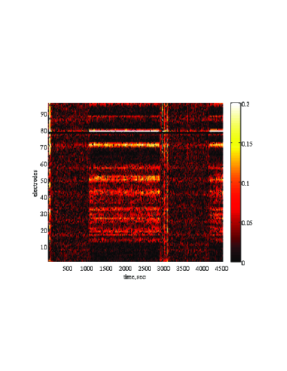
Figure 7: (Color online) A typical SSD for a focal electrode [here, F14 (i=78)]. The electrodes here are numbered and correspond to: 1-8 (AT1-AT8), 9-12 (ST1-ST4), 13-58 (P13-P58), 59-64 (PT3-PT8), 65-96 (F1-F32). The time span of the diagram is 1 hour 30 minutes.

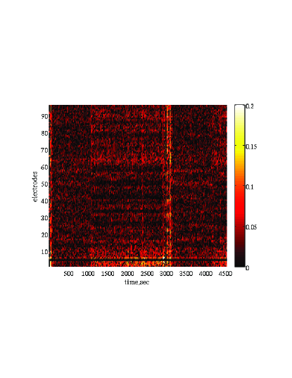
Figure 8: (Color online) A typical SSD for a non-focal electrode [here, AT5 (i=5)]. Electrodes are numbered as in Fig. 7. The time span of the diagram is 1 hour 30 minutes.

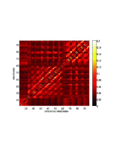
Figure 9: (Color online) A typical mean pair-wise synchronization matrix $\bar{S}_{i,j}$, computed from the same $S_{ij}$ as shown in Figs. 7 and 8, for the time interval (2000,2600) sec.

We refer to the diagram in which $S_{ij}(t)$ is displayed as the Strength of Synchronization Diagram (SSD). We color code the values of $S_{ij}(t)$ such that black is zero and white is the highest.

Two such typical diagrams [using as reference electrodes the specific electrodes F14 ($i=78$) and AT5 ($i=5$)] and $j$ from 1 to 96 are presented in Figs. 7 and 8. The diagrams correspond to a part of the record one and a half hour long, containing two subsequent seizures. The electrodes in these figures are numbered and correspond to: 1-8 (AT1-AT8), 9-12 (ST1-ST4),13-58 (P13-P58), 59-64 (PT3-PT8), 65-96 (F1-F32) (cf. Fig 2).

Note that a “strength of synchronization” of, say, 0.2, means that the signals are synchronized 20% of the time within the given time window.

The SSD provides a clear scenario of synchronization dynamics between these two seizures. The diagrams start with the final stages of the first seizure (ending at about $t\approx 20$ seconds) with a high synchronization strength in almost all channels. Then the synchronization is lost for about 15 minutes. It then reappears at $t\approx 1100$ seconds. In Fig. 7, showing SSD for the reference electrode F14, the most strong synchronization to the group of neighboring electrodes F6-8 ($i=70-72$), F15-16 ($i=79-80$) and F22-23 ($i=86-87$) is evident, while a larger group of electrodes is synchronized with F14 at lower strength. Interestingly, this electrode demonstrates similar level of synchronization strength with a spatially remote P grid, especially with electrodes P49-PG52 ($i=49-52$). At the same time, the electrode AT5 (Fig.8) becomes weakly synchronized with only few neighboring electrodes from the same strip. The next seizure occur between $t\approx 3000$ seconds and $t\approx 3240$ seconds. Starting around $t=2940$ with a decrease in synchronization the event proceeds to exhibit high synchronization between all the electrodes, starting around $t=3000$. After $t\approx 3240$ the synchronization is again lost and regained by F14 at about $t=4300$ seconds, as it did at $t\approx 1100$.

It is crucial to stress that the SSD patterns presented in Figs. 7 and 8 are qualitatively preserved over all seizures of the same patient in our data. Moreover, the groups of strongly synchronized electrodes are preserved throughout all records, although at varying strength. The desynchronization following the seizure, apparent in Figs. 7 and 8, corresponds to the post-ictal state, detected at the time of recording.

Similar behavior was found in the data of two other patients. In a patient A’s data only four pairs of electrodes remain synchronized during all available records. Two of these pairs were placed at the temporal lobe. During the seizures, a particularly strong synchronization was found in the signals coming only from AT and ST electrodes. For patient C three independent groups of strongly synchronized electrodes were found, while the overall behavior was similar to that of patient B.

III Results and Discussion

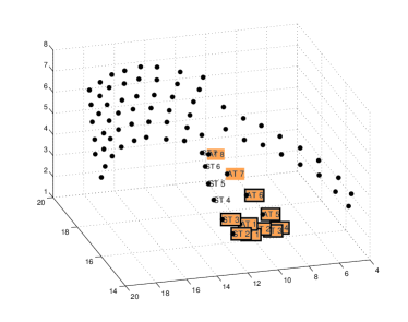
Figure 10: (Color online) The geometric spread of the electrodes, for the patient A. The viewing angle was chosen to best present the resected area. Only relevant electrodes are labeled. The electrodes with synchronization strength exceeding the threshold value $\bar{S}$ are marked by a rectangle. The electrodes chosen for resection are highlighted.

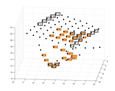
Figure 11: (Color online) The electrodes scheme for the patient C. The viewing angle was chosen to best present the resected areas. Only relevant electrodes are labeled for clarity. The electrodes are marked as in Fig 10.

Previous observations involving different linear and non-linear measures bia06 ; schevon ; towle99 ; doron06 ; quyen05 indicate that the values of the corresponding measures are altered over tumors and regions thought to be part of the epileptogenic zone. The regions of such a locally enhanced or suppressed activity are stable and have well defined edges. Since we found high synchronization strength during epileptic seizures, we identify the foci of epileptic activity with those regions that statistically preserve a high degree of synchronization at all times. Thus our definition of the foci of epileptic seizures is the ensemble of those electrodes that, besides being strongly synchronized to each other during the ictal period, remain also synchronized above a chosen threshold during the inter-ictal period. To identify this ensemble, we now compute the time average of $\bar{S}_{ij}$ according to

$$\bar{S}_{ij}\equiv T^{-1}\sum_{t_{k}=1}^{T}S_{ij}(t_{k})\ ,$$ (3)

where the time interval $(1,T)$ does not include a seizure. An example of the resulting mean pair-wise synchronization matrix $\bar{S}_{ij}$ is shown in Fig. 9. $\bar{S}_{i,j}$ converges well for $T>60$ seconds. Clearly, the synchronization strength between electrodes within a given grid is higher than between spatially remote electrodes. For a collection ${\cal E}_{\rm ref}$ of $N_{\rm ref}$ reference electrodes and a collection ${\cal E}_{\rm el}$ of $N_{\rm el}$ electrodes (cf. Fig. 9) we define the mean $\bar{S}$ as:

$$\bar{S}\equiv\frac{1}{N_{\rm el}N_{\rm ref}}\sum_{i\in{\cal E}_{\rm ref}}\sum_{j\in{\cal E}_{\rm el}}\bar{S}_{ij}\ .$$ (4)

For the diagram shown in Fig. 9, we calculated $\bar{S}$ and the standard deviation $\sigma$ of $\bar{S}_{ij}$ for each of five grids and between the grids. The value of $\bar{S}$ within the grid, averaged over five grids is $0.056$ (varying $0.047-0.065$ for different grids). The standard deviation $\sigma$ within the grid, averaged over five grids is $\sigma=0.034$ (ranging $0.03-0.042$ for different grids). The value of $\bar{S}$ averaged over all inter-grid combination of electrodes is $0.038$ (range $0.031-0.045$) within $\sigma=0.007$ (range $0.004-0.0125$). At the same time, the SS of the strongly synchronized group ranges in the interval $0.1-0.2$, being more than three standard deviations above the corresponding mean value. The difference is especially striking for the inter-grid synchronization, found between the group in F grid (F6-7, F14-16), and the remote group in P grid (P49, P50). These values are typical for all data of patient B, except for post-ictal periods. Similar values of $\bar{S}_{ij}$ were found for patients A and C, although no such remote synchronization was detected. This observation is consistent with the relations between values of mean phase coherence of the electrodes pairs that belong to the local hypersynchrony regions and those that are outside of these regions, found in schevon .

To localize the foci we need to choose a threshold value $\bar{S}_{\rm th}$, such that only electrode pairs with $\bar{S}_{ij}>\bar{S}_{\rm th}$ will be selected as belonging to the focus. Although for these pairs usually both $\bar{S}_{ij}$ and $\bar{S}_{ji}$ were above the threshold, we always used the largest of the two to compare with $\bar{S}_{\rm th}$. Clearly, the number of selected electrodes is a strong function of $\bar{S}_{\rm th}$. To compare with the actual selection we chose $\bar{S}_{\rm th}$, such that the number of electrodes designated by the present procedure agrees as much as possible with the number chosen by the epileptologists. It turned out that chosen values of $\bar{S}_{\rm th}$ are larger than the value of $\bar{S}$ by at least three standard deviations.

The results, that refer to calculations over the entire set of available data, are displayed in Figs. 2, 10 and 11. We color those electrodes that were chosen for the operation, and we put a rectangle on every electrode that is identified by our method.

For patient A, the SS was relatively low in the inter-ictal periods. On the other hand, during the seizure, the entire region, covered by AT and ST strips was synchronized at a level of 0.6-0.7. We included in the selection 9 electrodes, that showed highest pairwise synchronization. They all are placed within the resected area, see Fig. 10. This patient was seizure-free after the surgery.

We have shown in Figs 7-9 that patient B had two remote groups of electrodes that remained inter-ictally synchronized. As seen in Fig 2, the chosen subset of strongly synchronized electrodes overlap with both foci, resected during surgery. Out of 13 electrodes marked for resection, 9 were identified also by us. However, we have found also other electrodes, that belong to the same focus (in the frontal grid), as well as adjacent electrodes from the parietal grid. The outcome of the surgery was a improvement in patient’s condition, who however did not become seizure-free.

As for patient C (cf. Fig.11), the operated area and our chosen set of electrodes overlap only partially. Out of 30 electrodes marked by epileptologists, only 9 were chosen also by us. An additional strongly synchronized group was found at the edge of the parietal grid, indicating the possibility for another, not resected focus. After initial improvement, this patient did not benefit from the surgery.

In summary, we pointed out that a simple and computationally fast method to detect phase synchrony in ECoG signals was able to detect and localize the multiple foci of epilepsy. The method does not require any assumptions about the spectral features of the signal or the nature of the synchronization between the signals. The measurement of the synchronization strength from the synchrogram amounts to a straightforward count of the data points within a chosen interval. The synchronization scenario in the long recordings is characterized by repeated patterns from one seizure to the next one. For each patient, we found a subset of electrodes, that statistically preserve a high degree of synchronization at all times. These subsets overlap fully or partially with the areas chosen for resection. In patient B we correctly identified the existence of two distant foci. In patient C we also identified the presence of additional focus, not operated on. The overlap of the location of the electrodes identified by our method and the resected areas was consistent with the degree of surgery success.

Although it is not reasonable to draw any final conclusions on the basis of the study of only three patients, these observations suggest that this method may become a useful tool to help improve the outcome of the surgical treatment of epilepsy.

Aknowledgments

We thank Itai Doron and Tomer Gazit for fruitful discussions. This work was partially supported by a EU grant under the GABA project. S.B. acknowledges a visiting fellowship granted by the Yeshaya Horowitz Association through the Center for Complexity Science.

References

- (1) S.J. Schiff, Nature Medicine 4, 1117 (1998); B. Litt and J. Echauz, The Lancet Neurology 1, 22 (2002);
- (2) G.Wildman, K.Lehnertz, U. Urbach,and C.E.Elger, Epilepsia 41, 811, 2000;
- (3) K. Lehnertz, R.G. Andrzejak, J. Arnhold, T.Kreuz, F. Mormann, C. Reike, G. Wildman and C.E. Elger, J. Clin. Neurophysiol. 18, 209, 2001
- (4) P. Grassberger and I. Procaccia, Physica D 9 189, (1983), Phys, Rev. Lett. 50 346, (1983).
- (5) J. Arnhold, P. Grassberger, K. Lehnertz , C.E. Elger, Physica D 134 419 (1999).
- (6) M. Le Van Quyen C. Adam, M. Baulac, J. Martinerie, F. J. Varela, Brain Res. 792, 24, 1998; M. Le Van Quyen, J. Martinerie, C. Adam, F.J. Varela, Physica D 127 250,(1999).
- (7) R.G. Andrzejak, F. Mormann, G. Wildman, T. Kreuz, C.E. Elger, K. Lehnertz, Epilepsy Res., 69, 30, 2006
- (8) F. Takens, in: D.A. Rand, L.S. Young (Eds.), Lecture Notes in Mathematics, vol. 898, Springer, Berlin, 1981, p. 366.
- (9) C.J. Stam, Clinical Neurophysiology 116, 2266, 2005
- (10) C.J. Stam, B.W. van Dijk, Physica D163, 236 (2002).
- (11) R. Quian Quiroga, T. Kreuz and P. Grassberger, Phys. Rev. E66, 041904 (2002).
- (12) K. Schindler, H. Leung, Ch.E. Elger and K. Lehnertz, Brain 130, 65 (2007).
- (13) S. Bialonski and K. Lehnertz, Phys Rev E 74, 051909, 2006;
- (14) C.A. Schevon, J. Cappell, R. Emerson, J. Isler, P. Grieve, R. Goodman, G. Mackhann Jr., H. Weiner, W. Doyele, R. Kuzniecky, O. Devinsky, and F. Gilliam., NeuroImage 35, 140 (2007)
- (15) M. Paluš, V. Komárek, Z. Hrnčíř, and K. Štěrbová, Phys Rev E 63, 046211, 2001
- (16) M.G. Rosenblum, A.S. Pikovsky and J. Kurths, Phys. Rev. Lett. 76, 1804 (1996);
- (17) S. Boccaletti, J. Kurths, D.L. Valladares, G. Osipov and C.S. Zhou, Phys. Rep. 366, 1 (2002).
- (18) P.E. McSharry, L.A. Smith and L. Tarassenko, Nature Medicine 9, 241 (2003).
- (19) S. Schafer, M.G. Rosenblum, J. Kurths and H.H. Abel, Nature 392, 239 (1998).
- (20) J. Engel Jr, P.C. van Ness, T. B. Rasmussen, L.M. Ojemann (1993). Outcome with respect to epileptic seizures. In: J. Engel, Jr. (ed.), Surgical Treatment of the Epilepsies, 2nd ed. New York: Raven Press, pp. 609621.
- (21) V. L. Towle, R.K. Carder, L. Khorasani, D. Lindberg ,J. Clin. Neurophysiol. 16, 528, (1999)
- (22) I. Doron, E. Hulata, I. Baruchi, V. L. Towle and E. Ben Jacob Phys. Rev. Lett. 96 258101 (2006).
- (23) M. Le Van Quyen, J. Soss, V. Navarro, R. Robertson,M. Chavez, M. Baulac, J. Martinerie, Clinical Neurophysiology 116, 559 (2005)