Seeking for Simplicity in Complex Networks, and Its Consequences for Cascade Failures

Abstract

Complex networks can be understood as graphs whose connectivity deviates from those of regular or near-regular graphs, which are understood as being ‘simple’. While a great deal of the attention so far dedicated to complex networks has been duly driven by the ‘complex’ nature of these structures, in this work we address the identification of simplicity, in the sense of regularity, in complex networks. The basic idea is to seek for subgraphs exhibiting small dispersion (e.g. standard deviation or entropy) of local measurements such as the node degree and clustering coefficient. This approach paves the way for the identification of subgraphs (patches) with nearly uniform connectivity, therefore complementing the characterization of the complexity of networks. We also performed analysis of cascade failures, revealing that the removal of vertices in ‘simple’ regions results in smaller damage to the network structure than the removal of vertices in the heterogeneous regions. We illustrate the potential of the proposed methodology with respect to four theoretical models as well as protein-protein interaction networks of three different species. Our results suggest that the simplicity of protein interaction grows as the result of natural selection. This increase in simplicity makes these networks more robust to cascade failures.

The rise of the complex networks research area was ultimately motivated by the finding that graphs obtained from natural or human-made structures tended to present intricate connectivity when compared to regular (e.g. lattices and meshes) or nearly-regular graphs (e.g. Flory and Erdős-Rényi networks). Given their structured connectivity, complex networks have provided excellent models for several ‘complex’ real-world systems ranging from the Internet to protein-protein interaction (e.g. Boccaletti et al. (2006); da F. Costa et al. (2007)). Yet, the dicotomy between simplicity and complexity continues to provide the motivation for related investigations.

The purpose of the present work is precisely to develop means to identify simplicity and regularity in complex networks in order not only to obtain better characterization of such structures, but also to investigate how such features can affect respective dynamics such as cascade failures. More specifically, the motivation for finding regularities in complex networks includes but is not limited to the following issues: (1) the properties and distribution of regular patches can help the characterization, understanding and modeling of complex networks; (2) the presence of regular patches in a complex network may suggest a hybrid nature of that network (e.g. a combination of the regular and scale-free paradigms); and (3) regular patches can have strong influence on dynamical processes taking place on the network.

In graph theory, a regular graph is characterized by having all its nodes with exactly the same degree. However, such a definition is limited in the sense that it is still possible to obtain a large diversity of such ‘regular’ graphs. Figure 1 presents three examples of ‘regular’ graphs. All nodes in these graphs exhibit the same degree, equal to four. While the structures in (a) and (c) have more ‘regular’ connectivity, the graph in (b) looks rather irregular. Actually, even the structure in (c) has irregularities if we consider measurements such as the individual clustering coefficient. It is clear from such an example that identical node degree is not enough to ensure uniform connectivity.

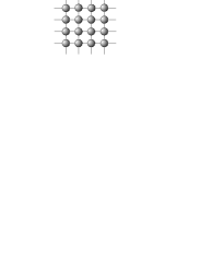
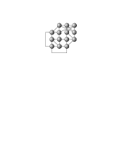
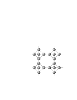
Figure 1: Three examples of ‘regular’ graphs, with all nodes with degree equal to 4.  

As we are interested in characterizing and identifying regularity (i.e. ‘simplicity’) in complex networks, the first important step consists of stating clearly what is meant by regularity, uniformity or simplicity. Perhaps the most strict imposition of regularity on a network is that every node would be undistinguishable from any other node whatever the considered measurements. Therefore, identical measurements (e.g. node degree, clustering coefficient, hierarchical degrees, etc.) would be obtained for any of the nodes in the perfectly regular network. In this sense, regularity becomes closely related to symmetries in the networks.

However, as we want to achieve increased flexibility, in this work we relax the above definition and propose that a graph (or subgraph) is regular whenever all its nodes present similar values for a set of measurements. Therefore, this definition is relative to the allowed degree of measurements dispersion, as well as the selection of the own set of measurements. Interestingly, traditional regularity in graph theory can be understood as a particular instance of the above definition in the case of null dispersion of node degree. Here we allow some tolerance for the variability of the measurements (e.g. in order to cope with incompleteness or noise during the network construction).

In order to characterize the local vertex structure, we considered the degree, clustering coefficient, neighboring degree and the locality index. The degree of each of any of its nodes $i$, henceforth abbreviated as $k(i)$, is defined as the number of immediate neighbors of $i$. The clustering coefficient of that node, represented as $cc(i)$, is calculated by dividing the number of edges between the immediate neighbors of $i$, i.e. $n_{E}(i)$, by the maximum possible number of connections between those nodes, i.e. $n_{E}(i)=k(i)(k(i)-1)/2$. The average neighboring degree $r(i)$ (e.g. Maslov and Sneppen (2002)) of a node $i$, corresponds to the average of the degrees of the immediate neighbors of $i$. The locality index $\mathrm{loc}(i)$ of a node $i$ corresponds to the ratio between the number of connections among the set of nodes comprising $i$ and its immediate neighbors divided by the sum of the edges connected to all those nodes Costa et al. (2006). This measurement has been motivated by the matching index Kaiser and Hilgetag (2004), which is adapted here in order to reflect the ‘internality’ of the connections of all the immediate neighbors of a given reference node, instead of a single edge.

In order to find the regular patches, the set of measurements defining homogeneity needs to be previously selected. Though such a set may include just the node degree (compatible with the traditional concept of regular graphs), because we want to impose more strict demands on regularity it is necessary to consider additional features describing the network connectivity around each node. Each vertex $i$ is represented by a vector with $M$ measurements, $X_{i}$, which is normalized da F. Costa et al. (2007) in order to have zero means and unit standard deviation. Then, the network, which is represented by the set of such vectors $X=\{X_{1},X_{2},\dots,X_{N}\}$ is projected into a two-dimensional space by considering principal component analysis – PCA (e.g. Duda et al. (2001); Johnson and Wichern (1988); da F. Costa and Jr. (2001); da F. Costa et al. (2007)). Such a statistical mapping implements a linear transformation (actually a rotation in the phase space) that ensures that the maximum dispersion of the points will be achieved along the initial projection axes (i.e. those corresponding to the largest absolute values of eigenvalues of the covariance matrix of the data). In addition, such a transformation optimally removes the redundancy of the data, which is fundamental in our analysis since local measurements are known to be correlated in most real-world networks Ravasz and Barabási (2003).

Having chosen the set of measurements and defined the projection, it is necessary to identify those nodes which are characterized by small dispersion of the measurements. Vertices with similar topological features tend to be mapped close one another in the two-dimensional space. However, visual inspection can provide inaccurate results because of the form of the distribution of points in the projection. Thus, we estimated the probability density in the 2D space by considering the non-parametric Parzen windows approach Parzen (1962); Duda et al. (2001). This method involves convolving the feature vectors (represented as Dirac’s deltas in the 2D projected space) with a two-variated Gaussian function (a normal distribution), allowing the interpolation of the probability density. In this way, high concentrations of points yield peaks in the probability density, which correspond to respective classes of vertices with homogeneous connectivity.

After determining the probability density of the node measurements as mapped into the two-dimensional projection, it is necessary to identify the obtained clusters of regular nodes. This is performed starting with the highest peak of the density. A cluster is created and associated to this peak, and its value is assigned to a control variable $V$. The value of $V$ is successively decreased and used to threshold the density, from which eventual new peaks are searched. In case a new peak appears, a new cluster is defined. Whenever two peaks merge, as a consequence of the progressive reduction of $V$, their respective clusters are subsumed, creating a branch in the hierarchical structure of clusters. When $V$ reaches its final value of 0, a tree representing the progressive merging of the peaks (and respective clusters) is obtained. The more significative clusters are identified by taking the clusters corresponding to the longest segments in the obtained tree.

However, the nodes defining a cluster do not necessarily correspond to a regular patch, as they might not be connected in the original graph. Therefore, the last step in the regular patch detection corresponds to obtaining the connected subgraphs for each considered homogeneous class in the distribution. Three indicators of the regularity of the network under analysis are considered in the current work: (i) the number of detected peaks $P$, (ii) the relative size of the maximum component identified considering all detected peaks, and (iii) index of dispersion of the measurements inside the largest regular region. The value of $P$ defines the number of different structures that can be found in the network. These structure can be thought of as generalized types of motifs, because they do not have regular pre-defined structures Milo et al. (2002), but are statistically similar. In order to compare results obtained for networks with different sizes, we define the simplicity coefficient as the the ration between the number of vertices in the largest connected region ($S$) and the network size ($N$),

$$\Sigma=\frac{S}{N}.$$ (1)

In addition, since the regularity can vary inside the largest regular region, we can define a super-regularity coefficient. The elements of the first eigenvector associated to the largest eigenvalue, $\vec{v}_{1}$, provide the dispersion of each respective measurement. Therefore, the level of regularity of the region can be quantified in terms of the coefficient of variation of the elements of such eigenvector, i.e. the super-regularity coefficient can be given by

$$\Gamma=\frac{\sigma_{\vec{v_{1}}}}{\langle\vec{v_{1}}\rangle}\left(\frac{1}{1+\frac{\sigma_{\vec{v_{1}}}}{\langle\vec{v_{1}}\rangle},}\right)$$ (2)

where $\langle\vec{v_{1}}\rangle$ is the average and $\sigma_{\vec{v_{1}}}$ is the standard deviation of $\vec{v_{1}}$. It can be shown that $0\leq\Gamma\leq 1$. Note that networks presenting values of $\Sigma$ and $\Gamma$ close to one tend to be highly regular regarding all the considered measurements.

We illustrate the above methodology by considering the network in Figure 2(a). First, a set of measurements is extracted and the vertices are projected into a two dimensional space. Note that the projection using principal component analysis is necessary only when more than two measurements are considered. We took into account two different configurations of measurements: (i) $M_{1}=\{k(i),cc(i)\}$, and (ii) $M_{2}=\{k(i),cc(i),r(i),loc(i)\}$. In the first case, the two main regular regions are composed by the vertices $R1=\{21,24,25,26,30,31,35,36,40,42,43,44\}$ and $R2=\{22,23,27,28,29,32,33,34,37,38,39\}$. While most of the vertices corresponding to region $R1$ belong to the border of the regular region of Figure 2(a), the vertices of $R2$ are internal to that region. In the latter case, i.e. considering a larger set of measurements, the connected main region corresponds to the vertices $R=\{22,23,24,26,27,28,29,30,31,32,33,34,35,36,37,38,39,\\ 40,41,42,43,44,45\}$, which forms the regular region presented in Figure 2(a). Our analysis of network models and real-world networks took into account these four local measurements.

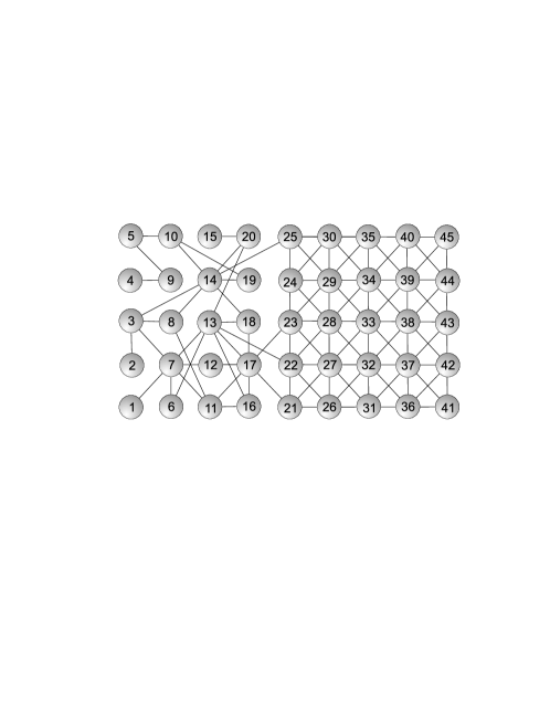
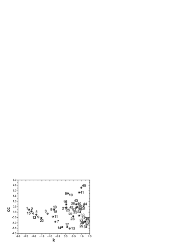
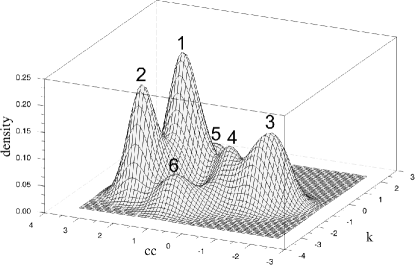
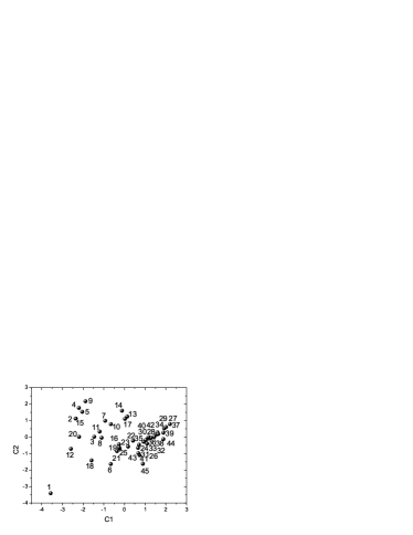
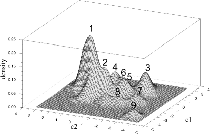
Figure 2: Illustration of the method to determine the simple patches in the network(a). (b) Distribution of the degree and cluster coefficient of each vertex and (c) the respective probability density function. The PCA projection of the measurements $M=\{k(i),cc(i),r(i),loc(i)\}$ into the two-dimensional space (d) and the respective probability density (e). The numbers in (c) and (e) indicate the order of the peaks, from the highest to the lowest.

In order to verify the importance of simple regions in networks under dynamic aspects, we considered the analysis of cascade failures. Cascade failures result in avalanche of breakdowns over the network when nodes and links are sensitive to overloading Motter and Lai (2002); Motter (2004). For a given network, a quantity of information (or energy) can be interchanged between pairs of nodes following the shortest paths distances at each time step. The capacity of a node $i$, $C_{i}$, is proportional to its initial load $L_{i}$, $C_{i}=(1+\alpha)L_{i}$, which is the maximum load that $i$ can handle. We represent the load $i$ by the betweenness centrality Motter and Lai (2002); Motter (2004). When a single node is removed from the network, the dynamics of redistribution of flows starts over the network and cascades can be triggered. Indeed, such removals change the shortest paths between nodes and, consequently, the distribution of the loads, creating overloads on some nodes. For $\alpha=0$, it is guaranteed that at time $t=0$ no node is overloaded and the system is working properly. Larger values of $\alpha$ increase the capacity of nodes and reduce the chance of cascade breakdown.

The analysis of cascade fails is performed by monitoring the avalanches when a single node in the regular and irregular regions is removed, independently. The damage caused by a cascade is quantified in terms of the relative size $G$ of the largest component, $G=N_{f}/N$, where $N_{f}$ is the size of the largest component after the avalanche.

Figure 3 shows the value of $G$ when a single vertex is removed in the largest simple and non-simple (the remainder of the network) regions for the Erdős-Rényi (ER), Knitted (KT) Costa (2007), Barabási-Albert (BA) and Krapivsky-Redner (NL) (based on non-linear preferential attachment, $P_{i\rightarrow j}=k_{j}^{0.5}/\sum_{u}k_{u}^{0.5}$) Krapivsky and Redner (2001) theoretical network models. Each point in the scatterplot corresponds to an average of the relative size of the resulting component $G$ after removing of each vertex $i$ in the simple and non-simple regions.

As we can see, the removal of vertices in the simple region tends to cause smaller damage on the network than the removal of vertices in the heterogeneous region for all models. This property had already been observed considering the whole network, in which homogenous networks tend to be more robust under fails and target attacks Motter and Lai (2002); Motter (2004). Therefore, the simpler regions are fundamental to network robustness. In addition, the curves obtained for models with similar structures, as BA e NL, present similar behaviors. The same happens with the ER and KT network models — the latter corresponding to the most regular model in our analysis Costa (2007), which is reflected in Table 1.

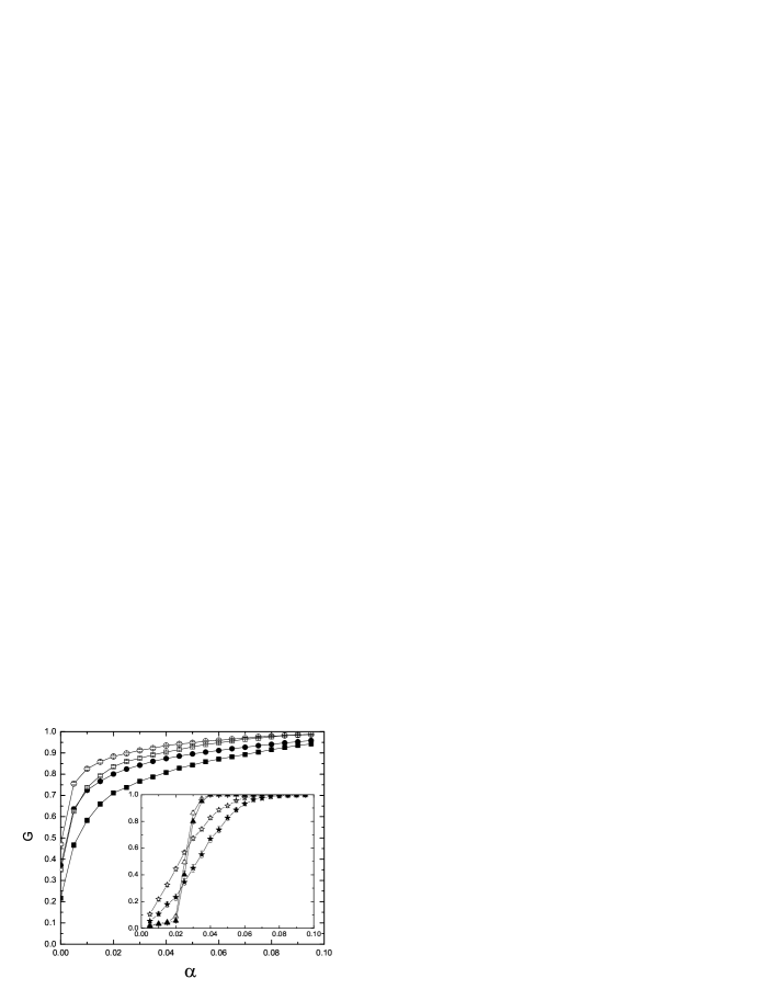
Figure 3: Cascading failure in BA (circles) and NL (squares) network models, and in ER (stars) and KT (triangles) (in the inset). The removal of vertices in the simple regions are represented by white symbols and in the heterogeneous regions by black symbols. Each curve corresponds to an average of $G$ after removing every vertex in each region, while the errors bars represent the standard deviations.

The protein databases were obtained from the Biogrid repository for protein interactions Stark et al. (2006). The analysis of the protein-protein interaction networks of the progressively more evolved species Sacharomyces cerevisiae, Drosophila melanogaster and Homo sapiens allowed us to investigate how the simplicity of the connections has changed during evolution under natural selection. As we can see in Table 1, the level of simplicity clearly increases with evolution — the protein interaction network of the H. sapiens is the most regular. The super-regularity coefficient also increases with the complexity of the organism. A possible explanation of this remarkable phenomena is related to protein evolution. Since hubs tend to evolve more slowly than less connected proteins, because they are more important in the organism, the addition of new connections due to mutation and duplication tend to favor the proteins that are not hubs, therefore increasing regularity Fraser et al. (2002). This process implies that more robust networks are obtained for more complex organisms. Considering the cascade effect on the protein interaction networks, we observed that the removal of vertices in regular region tends to be less destructive than removal in the non-regular region, as also observed for the BA and NL network models in Figure 3.

While analyzing the effect of the regularity on the largest regular regions in BA, NL and the three protein-protein interaction networks, which are scale-free networks, we observed that there is a positive correlation between the super-regularity coefficient and the average of the relative size $G$ of the largest component for $0\leq\alpha\leq 0.1$ — the obtained Pearson coefficient is 0.7. This indicates that the more regular the regions, the more robust they are under removal of vertices in such regions. Moreover, we investigated the effect of the variation of each four considered measurements ($k(i),cc(i),r(i)$ and $loc(i)$) and observed that each of them is correlated to the average of the relative size $G$. Therefore, we can conclude that the smaller the variation of the local measurements inside the largest regular region, the more robust the network is with respect to the cascade dynamics. This is a consequence of the homogeneous distribution of shortest paths in such regions — as the vertices tend to have similar properties, their betweenness centrality becomes similar. This effect was identified in every considered networks. Indeed, vertices with the highest betweenness tend to be outside the regular regions, since such vertices generally present distinct local properties (such as the hubs). These vertices tend to be the outliers in the PCA projection.

Table 1: The simplicity in different networks.

Network	$N$	$\langle k\rangle$	$\langle cc\rangle$	$P$	$\Sigma$	$\Gamma$
S. cerevisiae	5439	28.4	0.20	24	0.13	0.44
D. melanogaster	7286	6.84	0.02	38	0.54	0.47
H. Sapiens	8792	7.13	0.07	32	0.75	0.60
Barabási-Albert	1000	8	0.04	34	0.45	0.34
Krapivsky-Redner	1000	8	0.02	30	0.50	0.36
Erdős-Rényi	1000	8	0.01	25	0.60	0.43
Knitted	1000	8	0.01	10	0.70	1.0

The reported method for identifying regular subgraphs (or patches) within complex networks, as well as the respectively obtained results, illustrated and corroborated the importance of considering patchwise regularity in order to characterize and obtain insights about the properties of theoretical and real-world networks. Several are the possibilities for further investigations opened by this work, which include but are not limited to the consideration of other real-world networks, selection of additional topological measurements, and analysis of evolution of simplicity in some biological networks, as the brain, food webs and genetic networks. In addition, our methodology can be applied to the identification of more general types of motifs, defined by similar structures. These motifs may not have fully regular structure, as defined currently Milo et al. (2002), but be characterized by statistically uniform properties.