Sivashinsky equation in a rectangular domain

Abstract

The (Michelson) Sivashinsky equation of premixed flames is studied in a rectangular domain in two dimensions. A huge number of 2D stationary solutions are trivially obtained by addition of two 1D solutions. With Neumann boundary conditions, it is shown numerically that adding two stable 1D solutions leads to a 2D stable solution. This type of solution is shown to play an important role in the dynamics of the equation with additive noise.

I Introduction

The Sivashinsky equation Sivashinsky (1977) (or Michelson Sivashinsky equation depending on the authors) is a non linear equation which describes the time evolution of premixed flames. Because of the jump of temperature (and thus of density) across the flame, a plane flame front is submitted to a hydrodynamic instability called the Darrieus-Landau instability. The conservation of normal mass flux and tangential velocity across the front leads to a deflection of streamlines which is the main cause of this instability. A more detailed description of this instability can be found in the book of Williams Williams (1985) (see also, in the approximation of potential flow in the burnt gases, the elementary electrostatic explanation in Denet (2002), where essentially the flame is described as a surface with a uniform charge density). At small scales, the instability is damped by diffusive effects: the local front propagation velocity is modified by a term proportional to curvature, the coefficient ahead of the curvature term is called the Markstein length. A geometrical non linear term, which limits ultimately the growth of the instability, is caused by the normal propagation of the flame. The Sivashinsky equation, obtained as a development in powers of a gas expansion parameter, i.e. for a small jump of temperature, or equivalently for a flow almost potential in the burnt gases, represents a balance between the evolution due to these three effects, Darrieus Landau instability, stabilization by curvature and normal propagation of the flame.

The qualitative agreement between the Sivashinsky equation and direct numerical simulations, generally performed with periodic boundary conditions has been excellent even with large gas expansion Rastigejev and Matalon (2006), and also when gravity is included Denet and Bonino (1994). It has been shown in a classic paper of the field Thual et al. (1985) (following Lee and Chen (1982), where the pole decomposition was introduced) that the 1D solution of the Sivashinsky equation in the absence of noise was attracted for large times toward stationary solutions, with poles aligned in the complex plane, called coalescent solutions. It was shown analytically in Vaynblatt and Matalon (2000a)Vaynblatt and Matalon (2000b) that each solution, with a given number of poles, is linearly stable in a given interval for the control parameter (either the domain width or more often the Markstein length with a domain width fixed to $2\pi$).

In a recent paper Denet (2006) (hereafter called I) the present author has been interested in the behavior of the Sivashinsky equation in 1D, but with Neumann boundary conditions (zero slope at each end of the domain), a situation which, although more realistic than periodic boundary conditions, had not attracted much interest over the years. Actually, periodic boundary conditions lead to a symmetry which is not present in the case of a flame in a tube, i.e. every lateral translation of a given solution is also a solution. Presented in a different way, a perturbation on the flame can grow, reach the cusp (the very curved part of the front, pointing toward the burnt gases) and then decay, but after having caused a global translation of the original solution. This is not possible with Neumann boundary conditions, but it was supposed that this difference with periodic boundary conditions was unimportant. The surprise was however that stable stationary solutions in the Neumann case involved a number of solutions with two cusps (and the corresponding poles) at each end of the domain, called bicoalescent solutions. This type of solution of the Sivashinsky equation was already introduced in Guidi and Marchetti (2003), although this last article did not obtain those which are stable with Neumann boundary conditions. The author would like to mention here two articles which he did not cite in I , namely Gutman and Sivashinsky (1990), where some bicoalescent solutions with Neumann boundary conditions were first obtained, and Travnikov et al. (2000) where bicoalescent solutions were obtained in direct numerical simulations. In this last paper, one solution was not completely stationary, because of the effect of noise, but another solution was actually almost stationary. Of course the computer time needed for such a simulation is probably one hundred times more than the equivalent Sivashinsky equation simulation, with all sorts of possible sources of noise, so obtaining really stationary bicoalescent solutions in this case is a challenging task.

Coming back to I, we can summarize the 1D results of this paper in the following way:

1. Bicoalescent solutions were obtained, stable with Neumann boundary conditions. Simulations performed without noise tend to these solutions.

2. The new solutions led to a bifurcation diagram with a large number of stationary solutions, where particularly the number of solutions multiply when the Markstein length, presented above, which controls the stabilizing influence of the curvature term, decreases

3. The bicoalescent solutions play a major role in the dynamics of the equation with additive noise. In the case of moderate white noise, the dynamics is controlled by jumps between different bicoalescent solutions.

In the present paper, we shall be interested in the Sivashinsky equation with Neumann boundary conditions, but in two dimensions in a rectangular domain. Another nice property of the equation (apart from the pole decomposition in 1D) is that 2D solutions can be formed by the simple addition of two 1D solutions, one for each coordinate Joulin (1996). The exact counterpart of I will be obtained:

1. Sums of two bicoalescent solutions are stable in 2D with Neumann boundary conditions. The time evolution of the equation without noise tends toward these solutions

2. With sums of a large number of 1D solutions, a really huge number of 2D solutions can be obtained.

3. The sums of bicoalescent solutions play also a major role in the dynamics in two dimensions in the presence of noise.

II Solutions in elongated domains

The Sivashinsky equation in one dimension can be written as

$$\phi_{t}+\frac{1}{2}\phi_{x}^{2}=\nu\phi_{xx}+I\left(\phi\right)$$ (1)

where $\phi\left(x\right)$ is the vertical position of the front. The Landau operator $I\left(\phi\right)$ corresponds to a multiplication by $\left|k\right|$ in Fourier space, where $k$ is the wavevector, and physically to the destabilizing influence of gas expansion on the flame front (known as the Darrieus-Landau instability, and described in the introduction). $\nu$ is the only parameter of the equation (the Markstein length) and controls the stabilizing influence of curvature. The linear dispersion relation giving the growth rate $\sigma$ versus the wavevector is, including the two effects:

$$\sigma=\left|k\right|-\nu k^{2}$$ (2)

As usual with Sivashinsky-type equations, the only non linear term added to the equation is $\frac{1}{2}\phi_{x}^{2}$. In the flame front case, this term is purely geometrical : the flame propagates in the direction of its normal, a projection on the vertical ($y$) direction gives the factor $\cos\left(\theta\right)=1/\sqrt{1+\phi_{x}^{2}}$, where $\theta$ is the angle between the normal and the vertical direction, then a development valid for small slopes of the front leads to the term $\frac{1}{2}\phi_{x}^{2}$. The Sivashinsky equation is typically solved numerically on $[0,2\pi]$ with periodic boundary conditions. In I it has also been solved on $[0,2\pi]$ with only symmetric modes, which corresponds to homogeneous Neumann boundary conditions on $[0,\pi]$ (zero slope on both ends of the domain). The two dimensional version of the Sivashinsky equation is

$$\phi_{t}+\frac{1}{2}\left(\nabla\phi\right)^{2}=\nu\Delta\phi+I\left(\phi\right)$$ (3)

where the Landau operator $I\left(\phi\right)$ corresponds now to a multiplication by $\sqrt{k_{x}^{2}+k_{y}^{2}}$ in Fourier space, $k_{x}$ and $k_{y}$ being the wavevectors in the $x$ and $y$ directions. All dynamical calculations, are performed by Fourier pseudo-spectral methods (i.e. the non linear term is calculated in physical space and not by a convolution product in Fourier space). The method used is first order in time and semi-implicit (implicit on the linear terms of the equation, explicit on $\frac{1}{2}\phi_{x}^{2}$). No particular treatment of aliasing errors is used. The 2D Sivashinsky equation is solved in $[0,2\pi]*[0,2b]$ with only symmetric modes, which corresponds to homogeneous Neumann boundary conditions in the rectangular domain $[0,\pi]*[0,b]$ .

Pole solutions (Thual et al. (1985)) of the 1D Sivashinsky equation are solutions of the form:

$$\phi=2\nu\sum_{n=1}^{N}\left\{\ln\left(\sin\left(\frac{x-z_{n}(t)}{2}\right)\right)+\ln\left(\sin\left(\frac{x-z_{n}^{*}(t)}{2}\right)\right)\right\}$$ (4)

where $N$ is the number of poles $z_{n}(t)$ in the complex plane. Actually the poles appear in complex conjugate pairs, and the asterisk in Equation 4 denotes the complex conjugate. In all the paper, the number of poles will also mean number of poles with a positive imaginary part. The pole decomposition transforms the solution of the Sivashinsky equation into the solution of a dynamical system for the locations of the poles. In the case of stationary solutions, the locations of the poles are obtained by solving a non linear system:

$$-\nu\sum_{l=1,l\neq n}^{2N}\cot\left(\frac{z_{n}-z_{l}}{2}\right)-i\textnormal{sgn}\left[{\textstyle\textnormal{Im}}\left(z_{n}\right)\right]=0\;\;\;\;\;n=1,\cdots,N$$ (5)

where $\textnormal{Im}\left(z_{n}\right)$ denotes the imaginary part and sgn is the signum function. This non linear system is solved by a variant of Newton method.

With periodic boundary condition, the usual result is that in the window $2n-1$$\leq 1/\nu$$\leq 2n+1$, $n=1,2,\cdots$ there exists $n$ different monocoalescent stationary solutions (all the poles have the same real part), with $1$ to $n$ poles, and the solution with the maximum number of poles $n$ is asymptotically stable. For a particular value of $1/\nu$, the number $n(\nu)$ such that $2n-1$$\leq 1/\nu$$\leq 2n+1$ is called the optimal number of poles.

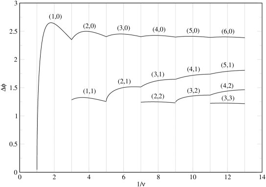
Figure 1: Stable stationary solutions in 1D: amplitude $\Delta\phi$ vs $1/\nu$. All the different branches are only plotted for the values of $1/\nu$ where they are stable. A notation like (3,2) means that 3 poles are located at $x=0$, and 2 poles at $x=\pi$

With Neumann boundary conditions, in each of the intervals $\left[2n-1,2n+1\right]$ of the parameter $1/\nu$, not only one asymptotically stable solution, but $n+1$, of the form $\left(l,n-l\right)$ with $l=0,1,$$\cdots,n$ where $l$ poles coalesce at $x=0$ and $l-n$ coalesce at $x=\pi$, were obtained in I. (The bicoalescent type of solutions have been recently introduced in Guidi and Marchetti (2003)). In Figure 1 is shown a bifurcation diagram with all the possible stable stationary solutions (plotted only, contrary to I, in the domain where they are stable) versus $1/\nu$. What is actually plotted is the amplitude $\Delta\phi$ (maximum minus minimum of $\phi$) versus $1/\nu.$ As can be seen, when the optimal number of poles increases with $1/\nu$, the number of stable stationary bicoalescent solutions is also increasing. The stability of these solutions is not proved analytically, nor by a numerical study of the linearized problem, we use only numerical simulations of the Sivashinsky equation, with the different bicoalescent solutions plus some small perturbations as initial conditions, and the solution returns toward the unperturbed solution.

In a square domain $[0,2\pi]*[0,2\pi]$, it has been remarked in Joulin (1996) that if $\phi_{1}(x)$ and $\phi_{2}(x)$ are solutions of the 1D Sivashinsky equation (1), then $\phi_{1}(x)+\phi_{2}(y)$ (we use here $\phi_{1}\oplus\phi_{2}$ as a notation for this sum, whose amplitude is the sum of the amplitudes of $\phi_{1}$ and $\phi_{2}$) is a solution of (3) in two dimensions, and that the stationary solution obtained numerically in this case for periodic boundary conditions Michelson and Sivashinsky (1982) is simply a sum of two monocoalescent 1D solutions. Let us note that, if it is absolutely obvious that sums are solutions of the 2D equation, the stability of these solutions has never been proved analytically, and can only be inferred from a small number of numerical simulations.

In the case of rectangular domains $[0,2\pi]*[0,2b]$, sums are also solutions of the equation, with $\phi_{2}$ now solution of the 1D Sivashinsky equation with parameter $1/\nu$ in domain $[0,2b]$, which can be obtained by an appropriate rescaling from the solution in $[0,2\pi]$ with parameter $1/\nu_{1}=(1/\nu)(b/\pi)$.

A particularly simple case is the limit where $b$ is very small, where the only solution with parameter $1/\nu$ in domain $[0,2b]$ is simply the flat $(0)$ solution $\phi_{2}=0$. As a sum of the previously described bicoalescent solutions in $[0,2\pi]$ added to the flat solution in the other direction, we have simply a way to observe the bicoalescent solutions in two dimensions. We have observed numerically (not shown here, the behavior is very similar to the 1D case) for Neumann boundary conditions, that these sums $\left(l,n-l\right)\oplus(0)$ are stable . As an example, for $1/\nu=10$ and $b=\pi/10$ we show in Figure 2 a perspective view of the three different stationary bicoalescent solutions $\left(5,0\right)\oplus(0)$, $\left(4,1\right)\oplus(0)$, $\left(3,2\right)\oplus(0)$ (from top to bottom). In all the figures, the whole domain $[0,2\pi]*[0,2b]$ is plotted, the solution with Neumann boundary conditions corresponds only to one fourth of the domain $[0,\pi]*[0,b]$ . We have found it clearer to show the whole domain (contrary to I), because some solutions are very difficult to distinguish if plotted in $[0,\pi]*[0,b]$. Although these solutions are very sensitive to noise (although less than the pure 1D solutions) it could be possible to observe in direct numerical simulations and experimentally the solutions with the lower amplitude, which are the least sensitive to noise. In experiments, the solutions should also survive heat losses (important in narrow channels) and not be too much perturbed by gravity (i.e. have a large enough Froude number) in order to be observed .

III solutions in square domains

We now turn to stationary solutions in square domains $[0,2\pi]*[0,2\pi]$ with Neumann boundary conditions. Sums of bicoalescent solutions produce also in this case stable stationary solutions. The purpose of this section is to give details on the consequences of this simple addition property. We show first the different types of solutions obtained by addition of stable bicoalescent solutions in 1D. We insist on the fact that these solutions are linearly stable and give a specific example of the time evolution of one such solution with some small perturbations. Finally two bifurcation diagrams are provided, one is the 2D equivalent of Figure 1 with the stable solutions plotted only in their stable domain. The second contains all the solutions obtained by addition of all the branches found in 1D in I, and as the reader will see, a really huge number of branches are created in this way.

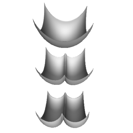
Figure 3: Perspective view of the (from top to bottom) $\left(5,0\right)\oplus(5,0)$, $\left(5,0\right)\oplus(4,1)$, $\left(5,0\right)\oplus(3,2)$ stationary solutions for $1/\nu=10$. The solution is plotted in the interval $[0,2\pi]*[0,2\pi]$ because it is easier to visualize. Actually, Neumann boundary conditions are satisfied in $[0,\pi]*[0,\pi]$ (one fourth of the domain shown).

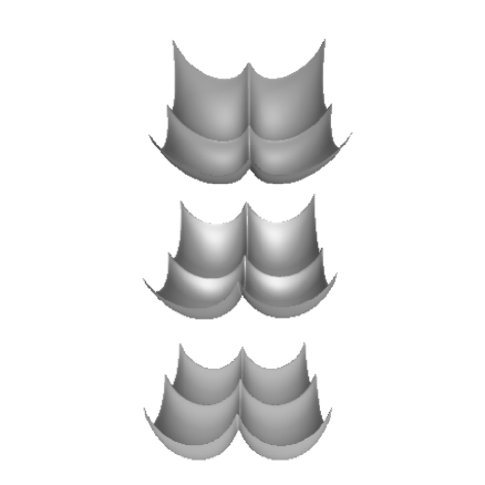
Figure 4: Perspective view of the (from top to bottom) $\left(4,1\right)\oplus(4,1)$, $\left(4,1\right)\oplus(3,2)$, $\left(3,2\right)\oplus(3,2)$ stationary solutions for $1/\nu=10$. The solution is plotted in the interval $[0,2\pi]*[0,2\pi]$ because it is easier to visualize. Actually, Neumann boundary conditions are satisfied in $[0,\pi]*[0,\pi]$ (one fourth of the domain shown).

In Figures 3 and 4 are shown the six stable solutions obtained from the three 1D solutions of Figure 2 for $1/\nu=10$. In Figure 3 can be seen (in perspective view, for the whole domain $[0,2\pi]*[0,2\pi]$), from top to bottom the $\left(5,0\right)\oplus(5,0)$, $\left(4,1\right)\oplus(5,0)$and $\left(3,2\right)\oplus(5,0)$ solutions. In Figure 4 can be seen the three remaining solutions $\left(4,1\right)\oplus(4,1)$, $\left(3,2\right)\oplus(4,1)$ and $\left(3,2\right)\oplus(3,2)$. All these solutions are found to be linearly stable, although all the solutions of Figure 3 ($(5,0)\oplus$ something) are extremely sensitive to noise. It must be pointed out that most of these solutions would have been almost impossible to find from a time integration of the 2D Sivashinsky equation (Equation (3)) because of this sensitivity to noise, and it is likely that obtaining them from a steady version of (3) would have been very difficult too.

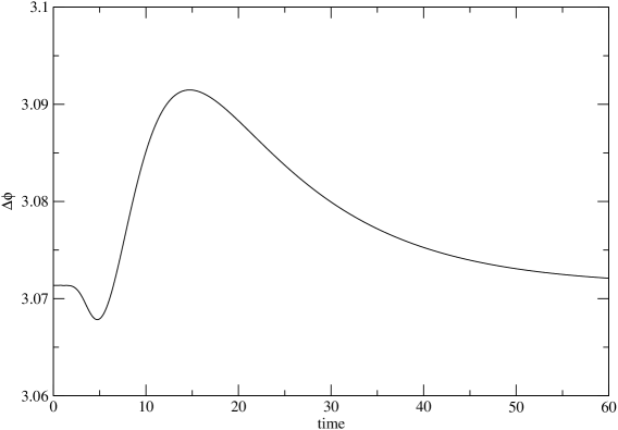
Figure 5: Amplitude vs time for $1/\nu=10$ , starting from a $(4,1)\oplus(3,2)$ solution. A gaussian white noise (amplitude $a=0.001$ ) is imposed on this solution when time is smaller than $0.5$. The solution returns exponentially toward the initial solution.

In Figure 5, we have an example showing the stability of the $\left(3,2\right)\oplus(4,1)$ solution. We start from this solution and add an additive white noise to Equation (3) when the time is below $0.5$. This white noise is gaussian, of deviation one, and we multiply it by an amplitude $a=0.001$. It can be seen that after the noise is stopped, the solution tends exponentially back toward the $\left(3,2\right)\oplus(4,1)$ solution. Similar figures would be obtained with the other solutions of Figures 3 and 4, except that higher amplitude solutions would need an even lower noise in order not to jump immediately toward a lower amplitude solution.

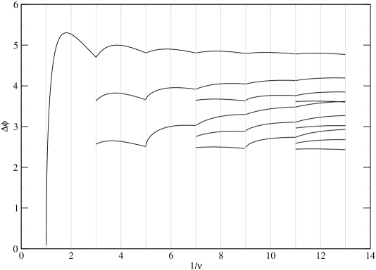
Figure 6: Stable stationary solutions in 2D for a square domain : amplitude $\Delta\phi$ vs $1/\nu$. All the different branches are only plotted for the values of $1/\nu$ where they are stable. The 2D linearly stable solutions are obtained by addition of the corresponding 1D linearly stable solutions of Figure 1.

In Figure 6 is shown the strict 2D equivalent of Figure 1: the bifurcation diagram showing the amplitude versus $1/\nu$ for all the solutions which are linearly stable, only plotted in their domain of stability. For $1/\nu<3$ there is only one possibility $\left(1,0\right)\oplus(1,0)$. For $3<1/\nu<5$ we have three branches (from higher to lower amplitudes) $\left(2,0\right)\oplus(2,0)$ $\left(1,1\right)\oplus(2,0)$ and $\left(1,1\right)\oplus(1,1)$. For the value $1/\nu=10$ we have the six solutions of Figures 3 and 4, that is from higher to lower amplitudes the $\left(5,0\right)\oplus(5,0)$, $\left(4,1\right)\oplus(5,0)$ $\left(3,2\right)\oplus(5,0)$ $\left(4,1\right)\oplus(4,1)$, $\left(3,2\right)\oplus(4,1)$ and $\left(3,2\right)\oplus(3,2)$ solutions. Higher values of $1/\nu$ would correspond to an increasing number of stable stationary solutions.

Naturally, neither Figure 1 (in 1D) or Figure 6 (in 2D) contain all the possible stationary solutions. In 1D Guidi and Marchetti Guidi and Marchetti (2003) have introduced the concept of interpolating solutions, which are unstable solutions connecting different branches of stable solutions in the previous bifurcation diagrams. In I, the present author has shown that this leads to a complex network of solutions, which was called web of stationary solutions. But now in two dimensions, we have the possibility, when two branches $\phi_{1}$ and $\phi_{2}$ exist for a parameter $1/\nu$ to create the 2D branch $\phi_{1}\oplus\phi_{2}$. This construction leads to a bifurcation diagram (with as before $1/\nu<14$, i.e. not very large flames) with a truly huge number of different stationary solutions (several thousands of branches). The comparison with Figure 6 shows that most of these solutions are linearly unstable.

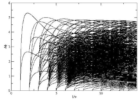
Figure 7: Stationary solutions in 2D for a square domain : amplitude $\Delta\phi$ vs $1/\nu$ (figure with all the solutions obtained by addition of 1D stationary solutions). When two 1D branches found in I coexist for a certain value of $1/\nu$, a 2D branch is created, whose amplitude is the sum of the 1D amplitudes.

The author would like to insist here on different points. First, it is only possible to obtain such an incredible number of stationary solutions because of two properties of the Sivashinsky equation, the pole decomposition, which transforms the search of stationary solutions in one dimension in a 0D problem, then the possibility to add 1D solutions in order to get 2D rectangular solutions of the Sivashinsky equation. In the Kuramoto-Sivashinsky equation case (a non linear equation with a different growth rate but the same non linear term) the pole decomposition is not available, but nevertheless a lot of 1D stationary solutions have been obtained Greene and Kim (1988). The Kuramoto-Sivashinsky equation shares with the Sivashinsky equation the possibility to create 2D solutions by adding two 1D solutions, so actually in this case we have also a very large number of branches. These rectangular solutions are not as physically relevant in the Kuramoto-Sivashinsky equation case. Contrary to the Sivashinsky equation, where stable stationary solutions are basically as large as possible and are thus rectangular in a rectangular domain, it seems likely that in the Kuramoto-Sivashinsky case, the most interesting solutions would have an hexagonal symmetry (hexagonal cells are also observed for the Sivashinsky equation with stabilizing gravity Denet (1993)). Stationary solutions of the Sivashinsky equation with hexagonal symmetry should exist too, and the author conjectures that the order of magnitude of the number of solutions with hexagonal symmetry should be approximately the same as those with rectangular symmetry. Apparently there is no trivial way to construct hexagonal solutions, so unfortunately, until some progress is made, obtaining the hexagonal equivalent of Figure 7 is almost impossible. We have here an example emphasizing the fact that as the smoothing effect (viscosity, curvature, surface tension …) decreases, we are not able to generate correctly all the simple solutions of a given set of partial differential equations (Sivashinsky and Kuramoto-Sivashinsky equations, Navier Stokes …) even with the aid of computers.

IV evolution with noise

In the previous section we have shown numerically that the sums of linearly stable 1D bicoalescent solutions lead to linearly stable 2D solutions. However, even a linearly stable solution could have a very small basin of attraction. So in this section, we study the effect of noise on the solutions of the Sivashinsky equation in a square domain, with Neumann boundary conditions. The important solutions will be the solutions that are reasonably resistant to the applied noise.

This noise used here is simply an additive noise, added to the right-hand side of Equation (3). We choose the simplest possible noise, a white noise (in space and time), which is gaussian, has deviation one and is multiplied by an amplitude $a$. But contrary to Figure 5, this noise will be applied at each time step. We use in all the simulations presented the same parameter $1/\nu=10$, the stationary solutions corresponding to this parameter have been presented in the previous section. We recall that in I, for the one dimensional version of the Sivashinsky equation with moderate noise, the evolution was analysed in terms of jumps between the available bicoalescent stationary solutions. We would like to show here that in 2D, the sums of bicoalescent solutions also play an important role in the dynamics.

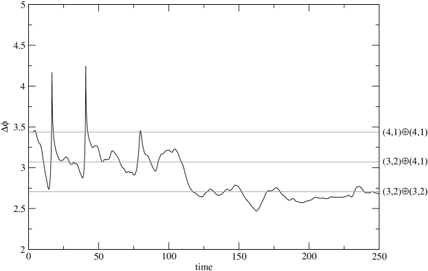
Figure 8: Amplitude vs time for $1/\nu=10$ and $a=0.01$ (low noise amplitude). Deexcitation from the $(4,1)\oplus(4,1)$ solution toward the $(3,2)\oplus(3,2)$ solution. This diagram suggests that the solution is first close to the $(3,2)\oplus(4,1)$ solution, then from the $(3,2)\oplus(3,2)$ solution, i.e. that the solution with the lowest amplitude is the most noise resistant.

In Figure 8, starting from an initial condition which is the $\left(4,1\right)\oplus(4,1)$ stationary solution, is plotted the amplitude of the solution versus time, for a noise amplitude $a=0.01$, with also straight lines corresponding to the amplitudes of the lowest amplitude stationary solutions, i.e. those of Figure 4. The stationary solutions with higher amplitudes (those of Figure 3) apparently are too sensitive to noise to play any role in the dynamics. It is seen in Figure 8 that because of the noise, the solution departs quickly from the $\left(4,1\right)\oplus(4,1)$ solution, and that it seems that, during the time evolution, the solution is close (apart from some violent peaks in the amplitude) to the $\left(3,2\right)\oplus(4,1)$ solution for some time, then finally the amplitude decreases again to be near that of the $\left(3,2\right)\oplus(3,2)$ solution.

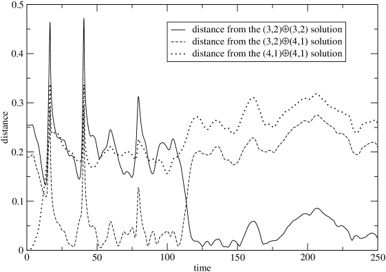
Figure 9: Distance to the main stationary solutions vs time for $1/\nu=10$ and $a=0.01$. A distance is a norm of the difference between the solution at a given time and the stationary solution. This diagram makes it possible to verify if a solution at a given time is indeed close to a stationary solution.

In order to prove that the solution is indeed close to the previously mentioned solutions, because after all very different solutions could have similar amplitudes, we plot in Figure 9 for the same simulation, what we have called the distance between the solution at a given time and the sums of bicoalescent solutions, which is simply the L1 norm of the difference between both solutions. The spatial mean value of all solutions is adjusted here to have the same value. Normally, it is necessary to measure the distance between the solution and all symmetries of a given sum of bicoalescent solutions (i.e. you can interchange the poles at $0$ and $\pi$ in the $x$ and $y$ directions) but for the low amplitude $a=0.01$, it has not been necessary, and we plot only the distance from the relevant solutions.

As we start from the $\left(4,1\right)\oplus(4,1)$ solution, the distance to this solution is zero initially, and we can see that, although the amplitude seems to indicate that at some time, one is again close to this solution, this is not the case. On the contrary, the solution returns regularly close to the $\left(3,2\right)\oplus(4,1)$ solution for times lower than $110$, then there is a transition toward something close to the $\left(3,2\right)\oplus(3,2)$ solution, the solution departs slightly from this last solution for some time, possibly toward a linearly unstable stationary solution, and returns toward it at the end of the simulation. As Figure 6 remotely looks like energy levels in atomic physics, one could be tempted to interpret the evolution of the two previous figures with a small noise (apparently in 2D the solution is less sensitive to a given amplitude of the white noise compared to 1D simulations) as a sort of deexcitation from the high amplitude level $\left(4,1\right)\oplus(4,1)$ toward first $\left(3,2\right)\oplus(4,1)$, then toward the fundamental level $\left(3,2\right)\oplus(3,2)$. Indeed, between the sums of bicoalescent solutions, if all are linearly stable, the solutions with the lower amplitude seems to be more resistant to the action of noise.

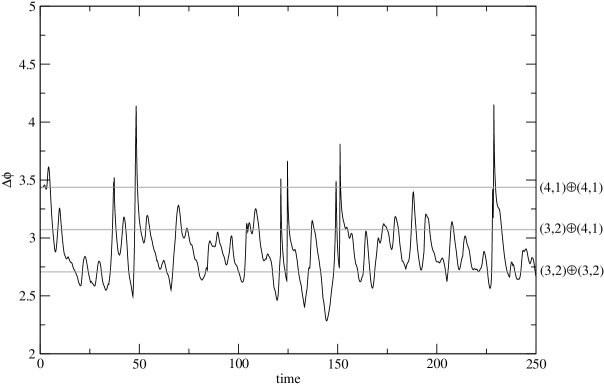
Figure 10: Amplitude vs time for $1/\nu=10$ and $a=0.1$ (moderate noise amplitude). This figure suggests that the solution is often close to the $(3,2)\oplus(3,2)$ solution. It will be shown in the following figures that it is close to the $(3,2)\oplus(4,1)$ solution only for times around $50$.

To better understand the effect of noise, we present now a simulation with a larger noise amplitude $a=0.1$ , ten times larger than the previous case (we recall that this noise amplitude should be compared to the laminar flame velocity, which is normalized to $1$ in this paper). In Figure 10 is plotted the amplitude versus time, with as before straight lines with the amplitude of the important sums of bicoalescent solutions. The initial condition is also the $\left(4,1\right)\oplus(4,1)$ solution. Apparently this last solution is too sensitive to noise to play a meaningful role in the dynamics, although it happens that some peaks in the amplitude could involve solutions not too far from this initial solution. As the distance to this solution is never really small, even in the peaks, we shall not comment further on this solution. On the other hand, it seems that a lot of time is spent with an amplitude close to that of the $\left(3,2\right)\oplus(3,2)$ solution (which we have called previously the fundamental level), and perhaps some time with an amplitude close to the $\left(3,2\right)\oplus(4,1)$ solution (the first excited level).

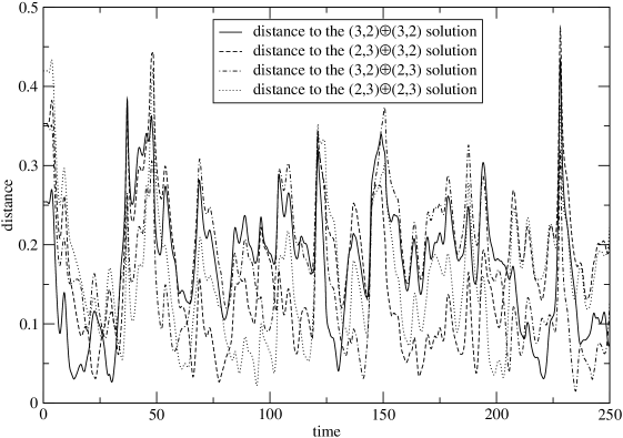
Figure 11: Distance to the different symmetries of the $(3,2)\oplus(3,2)$ solution vs time for $1/\nu=10$ and $a=0.1$. The noise is sufficiently large to induce transitions between the different symmetries of this fundamental level.

In order to see what is really occurring, we now turn to figures of the distance (defined above) to these two solutions versus time (for the same simulation of Figure 10). However, for a higher amplitude, we have to include the four different symmetries of these solutions in the analysis (i.e. for instance $\left(3,2\right)\oplus(4,1)$ $\left(3,2\right)\oplus(1,4)$ $\left(2,3\right)\oplus(4,1)$ $\left(2,3\right)\oplus(1,4)$ ) . In Figure 11 is shown the distance to the four symmetries of the $\left(3,2\right)\oplus(3,2)$ solution. The distance to one of the four symmetries is indeed often small (but not very small for this value of the noise) during the time evolution. Then because of the noise, perturbations are created that lead the amplitude to increase as the perturbation is convected toward one of the cusps, and the solution often comes back toward another symmetry of the fundamental level.

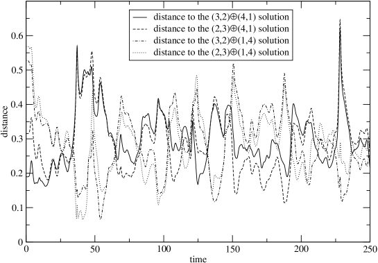
Figure 12: Distance to the different symmetries of the $(3,2)\oplus(4,1)$ solution (first excited level) vs time for $1/\nu=10$ and $a=0.1$. The solution is only close to one symmetry of the $(3,2)\oplus(4,1)$ solution for times around $50$ (after apparently a transition from a $(3,2)\oplus(3,2)$ solution).

In Figure 12 is shown the distance to the four symmetries of the $\left(3,2\right)\oplus(4,1)$ solution (the first excited level) (always for the same simulation). It is seen that the solution is only reasonably close to this type of solution at times close to $50$. At other times, minima of the distance are not very small and the solution is often closer to the $\left(3,2\right)\oplus(3,2)$ solution. In I, we have presented the evolution of the 1D Sivashinsky equation with a moderate additive noise as a series of jumps between bicoalescent solutions. In 2D the situation is relatively similar, with the sums of bicoalescent solutions playing the same role. However, the noise amplitude necessary to cause jumps seems much higher in 2D, and practically speaking during the previous simulation, only the fundamental (the solution with the lowest amplitude) and first excited levels were obtained. It should also be noted that the degenerescence (the four possible symmetries) of the fundamental level is probably important in the evolution (for instance for $1/\nu=12$ the fundamental level would be $\left(3,3\right)\oplus(3,3)$, which does not lead to other solutions by symmetry, so that it should be less likely to obtain the fundamental level in this case).

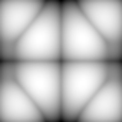
Figure 13: Solution at time $120.1$ for $1/\nu=10$ and $a=0.1$, plotted as a grayscale figure (white: minimum of $\phi$, black: maximum of $\phi$). The solution is plotted in the interval $[0,2\pi]*[0,2\pi]$. Presence of an oblique perturbation which has grown on a sum of bicoalescent solutions. This perturbation will reach one corner in the figure, be damped, and the solution will again be close to a sum of bicoalescent solutions.

Before closing this section, let us insist on the fact that, if the solution regularly returns toward sums of bicoalescent solutions, the fronts we obtain are not sums for each time. Figure 13, where is plotted a front of the previous simulation for time $120.1$ (just before a peak of the amplitude in Figure 10) , should be a clear example of this property. In this Figure, the whole domain $[0,2\pi]*[0,2\pi]$ is plotted as before, but this time as a grayscale figure, white corresponding to the minimum of $\phi$, black to the maximum. Essentially, an oblique perturbation has grown on a front that was previously a sum. This oblique perturbation moves toward each corner of Figure 13, and the amplitude peak corresponds to the moment where the perturbation reaches the corner. Then the solution is attracted again toward a sum of bicoalescent solutions.

To summarize this section on the effect of noise, the fact that all the sums of bicoalescent solutions with the optimal number of poles are linearly stable does not prove that they can be practically observed. On the contrary, the solutions with the larger amplitude have a basin of attraction so small that they can almost never be seen. We have introduced an analogy with atomic physics by calling the bicoalescent solution with the lowest amplitude the fundamental level, other solutions the excited levels. In the examples shown, only the fundamental and first excited levels (and their symmetries) were obtained during the time evolution of the Sivashinsky equation excited by an additive noise. We recall that in I, it was shown in 1D that the evolution with noise was completely different with periodic boundary conditions, where only the largest amplitude monocoalescent solution was linearly stable (even if extremely sensitive to noise). In this case, the solution regularly returns close to the highest amplitude solution. With Neumann boundary conditions, this is just the opposite, the solution prefers to be close to the lowest amplitude, almost symmetric, sum of bicoalescent solutions.

V conclusion

In this paper, we have used the possibility to create two dimensional rectangular stationary solutions from the addition of two 1D stationary solutions in order to generate a huge number of stationary solutions of the Sivashinsky equation. With Neumann boundary conditions, the addition of two stable 1D bicoalescent solutions leads to stable 2D solutions, which also play a role in the dynamics when an additive noise is added to the equation. However, with noise, only the sums of bicoalescent solutions with the lowest amplitude (which are less sensitive to noise) have a reasonable chance to be observed. More precisely, jumps between different symmetries of the lowest amplitude sum, or between the two sums with the lower amplitude, are obtained in the simulations. Although we have used a white noise in this paper, experiments, submitted to a residual turbulence, should behave in a similar way. In order to have a large enough Froude number for gravity effects to be negligible, flames with a sufficiently large laminar flame velocity would have to be chosen.

Figure 2: Perspective view of the (from top to bottom) $\left(5,0\right)\oplus(0)$, $\left(4,1\right)\oplus(0)$, $\left(3,2\right)\oplus(0)$ stationary solutions for $1/\nu=10$ and $b=\pi/10$. The solution is plotted in the interval $[0,2\pi]*[0,2b]$ because it is easier to visualize. Actually, Neumann boundary conditions are satisfied in $[0,\pi]*[0,b]$ (one fourth of the domain shown).

References

- Sivashinsky (1977) G. Sivashinsky, Acta Astronautica 4, 1117 (1977).
- Williams (1985) F.A. Williams, Combustion Theory (Benjamin Cummings, Menlo Park, CA, 1985).
- Denet (2002) B. Denet, Phys. Fluids 14, 3577 (2002).
- Rastigejev and Matalon (2006) Y. Rastigejev and M. Matalon, J. Fluid. Mech. 554, 371 (2006).
- Denet and Bonino (1994) B. Denet and J.L. Bonino, Combust. Sci. Tech. 99, 235 (1994).
- Thual et al. (1985) O. Thual, U. Frisch, and M. Hénon, J. Phys. France 46, 1485 (1985).
- Lee and Chen (1982) Y. Lee and H. Chen, Phys. Scr. 2, 41 (1982).
- Vaynblatt and Matalon (2000a) D. Vaynblatt and M. Matalon, Siam J. Appl. Math. 60, 679 (2000a).
- Vaynblatt and Matalon (2000b) D. Vaynblatt and M. Matalon, Siam J. Appl. Math. 60, 703 (2000b).
- Denet (2006) B. Denet, Phys. Rev. E 74, 036303 (2006).
- Guidi and Marchetti (2003) L. Guidi and D. Marchetti, Physics Letters A 308, 162 (2003).
- Gutman and Sivashinsky (1990) S. Gutman and G. Sivashinsky, Physica D 43, 129 (1990).
- Travnikov et al. (2000) O. Travnikov, V. Bychkov, and M. Liberman, Phys. Rev. E 61, 468 (2000).
- Joulin (1996) G. Joulin, Image des Mathématiques Modélisation de la combustion (CNRS, 1996), chap. Dynamique des fronts de flamme, p. 53.
- Michelson and Sivashinsky (1982) D. Michelson and G. Sivashinsky, Combustion and Flame 48, 211 (1982).
- Greene and Kim (1988) J. Greene and J. Kim, Physica D. 33, 99 (1988).
- Denet (1993) B. Denet, Combust. Sci. Tech. 92, 123 (1993).