Multi-directed Eulerian growing networks

Abstract

We introduce and analyze a model of a multi-directed Eulerian network, that is a directed and weighted network where a path exists that passes through all the edges of the network once and only once. Networks of this type can be used to describe information networks such as human language or DNA chains. We are able to calculate the strength and degree distribution in this network and find that they both exhibit a power law with an exponent between 2 and 3. We then analyze the behavior of the accelerated version of the model and find that the strength distribution has a double slope power law behavior. Finally we introduce a non-Eulerian version of the model and find that the statistical topological properties remain unchanged. Our analytical results are compared with numerical simulations.

I Introduction.

Many naturally occurring systems appear as chains of repeated elements. Such systems, such as human language, DNA chains, etc.., often encode and transport information. Markov processes have been adopted to model those chainsM . Unfortunately Markov chains are not able to describe long range correlations that exist within these structures. Thus complex growing networks appear to be a more suitable modeling tool.

In this paper we study written human language as a complex growing network. Since the discovery by Zipf 1 that language exhibits a complex behavior, and the application of Simon’s theories3 to growing networks4 , this topic has been examined by a number of scientists l1 ; l2 ; l3 ; l4 .

A useful way to build a network from a text is to associate a vertex to each sign of the text, that is both words and punctuation, and to put a link between two vertices if they are adjacent in the text. In a previous paper ap we showed that it is necessary to consider a directed and weighted network to understand the topological properties of this language network, in which the weight of each link in the network represents the number of directed links connecting two vertices. Directed links in such a network are necessary since they need to describe systems in which a syntax is defined and where attachments rules between the objects are not reflexives ap .

When networks are built in this way, from a chain of repeated elements, a weighted adjacency matrix is obtained that is well known graph in graph theory: the multi-Eulerian graphg . Eulerian means that there exists a path in the graph passing through all the links of the network once and only once, while the prefix:”multi” refers to the fact the adjacency matrix allows multiple links between two vertices.

In order to describe the evolution of a multi-directed graph we need to introduce the formalism of weighted networksw ; w1 . These are characterized by a weighted adjacency matrix $W=\{w_{ij}\}$ whose elements $w_{ij}$ represent the number of directed links connecting vertex $i$ to vertex $j$. We define the degree $k_{i}^{out/in}$ of vertex $i$ as the number of out/in-nearest neighbours of vertex $i$ and we have $k_{i}^{out/in}=\sum_{j}\Theta(w_{ij/ji}-\frac{1}{2})$. We define the out/in-strength $s_{i}^{out/in}$ of vertex $i$ as the number of outgoing/incoming links of vertex $i$, that is $s_{i}^{out/in}=\sum_{j}w_{ij/ji}$. Analytically the Eulerian condition means that the graph must be connected and it must have $s_{i}^{in}=s_{i}^{out}$ for every $i$.

In this work we first develop and analyze a model for a general multi-directed Eulerian growing network. Then, since human language is an accelerated growing network,we extend our model to its accelerated version, and find results similar to those in l1 . More recent works on accelerated growing networks can be find in p ; x . To conclude we introduce and analyze the non-Eulerian version of our model. This last step allows us to build a directed network without initial vertex attractiveness. As far as we are aware, this is the first time a model for directed networks has been proposed without the help of this ingredient. The resulting power laws exponents, tunable between $2$ and $3$, are very interesting since they fit with those found within most of the real networks4 ; d .

II Model A

First we introduce a model for the multi-directed Eulerian growing network which we will call $ModelA$. The Eulerian condition (hereafter EC) states that every newly introduced edge has to join the last connected vertex, so that every newly introduced in-link implies a constrained out-link from the last connected vertex. This is equivalent to say that $s_{i}^{in}=\sum_{j}w_{ij}=\sum_{j}w_{ji}=s_{i}^{out}=s$, for every $i$, with the global constraint the network must be connected (Fig.1). With the last condition our calculations become easier since we have to consider one quantity, that is $s$, instead of two.

We start with a chain of $2m$ connected vertices. At each time step we create a new vertex and $m+2$ new directed edges (Fig.1). At each time step

a- The new vertex will acquire one in-link with the constraint that the network must respect the EC.

b- The remaining $m+1$ in-links will be attached to old vertices with probability proportional to their in-strength with the constraint that the network must respect the EC.

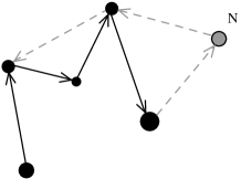
Figure 1: Growth mechanism for model A with $m=1$. Dashed grey arrows represent $m+2$ newly introduced edges.

To calculate the strength distribution for the model, we use the fact that with the EC the in-strength will be exactly the same as the out-strength distribution. We write the equation for the strength evolution $s(t,t_{i})$ at time $t$ for the vertex born at time $t_{i}$ as:

$$\frac{ds(t,t_{i})}{dt}=(m+1)\frac{s(t,t_{i})}{\sum_{i}s(t,t_{i})}.$$ (1)

The right hand side of the last equation takes into account that $m+1$ vertices acquire a link with probability proportional to their normalized strength $\frac{s_{i}}{\sum s_{i}}$. Considering that the total number of in/out-links at time $t$ is $\sum_{i}s(t,t_{i})=(m+2)t$ and integrating Eq.1 with the initial condition $s(t_{i},t_{i})=1$ we obtain

$$s(t,t_{i})=\left(\frac{t}{t_{i}}\right)^{\frac{m+1}{m+2}}.$$ (2)

Using the fact that

$$P(s,t)=-\frac{1}{t}\frac{\partial t_{i}}{\partial s(t,t_{i})}|_{s(t,t_{i})=s(t)}$$ (3)

from Eq.2 we obtain:

$$P(s,t)=\frac{m+2}{m+1}s^{-\frac{2m+3}{m+1}}$$ (4)

which is a stationary power-law distribution with exponent between $2$ and $3$. In particular it will be $3$ for $m=0$, and it will tend to $2$ for increasing values of $m$.

In order to calculate the degree distribution we consider that each time the strength of a vertex increases by 1, the degree of the vertex increases if and only if the vertex links with a new neighbor. This process implies higher order correlations. We will approximate this process as an uncorrelated one and compare our results with simulations. Hence the equation governing the evolution of the degree is

$$\frac{dk(t,t_{i})}{dt}=\left[1+m\left(1-\frac{k(t,t_{i})}{t}\right)\right]\frac{s(t,t_{i})}{\sum s(t,t_{i})}.$$ (5)

To understand this equation we have to notice that the degree of a vertex grows at a rate proportional to its normalized strength, as in Eq.2, but, when the strength of a vertex increases by 1, the probability that the degree of the vertex $i$ increases by 1 is $(1-k(t,t_{i})/t)$. In fact $k(t,t_{i})$ is the number of nearest neighbors of vertex $i$, while $t$ represents the total number of vertices at time $t$. Note that for $m=0$, $k(t,t_{i})=s(t,t_{i})$ as we would expect.

We substitute Eq.2 in Eq.5 and we integrate it to obtain

$$k(t,t_{i})=\frac{(m+1)m^{m+1}}{t_{i}^{m+1}}\exp{\left(\frac{mt^{-\frac{1}{m+2}}}{t_{i}^{\frac{m+1}{m+2}}}\right)}\left\{\Gamma\left[-(m+1),\frac{m}{t_{i}^{\frac{m+1}{m+2}}}t^{-\frac{1}{m+2}}\right]+C\right\}$$ (6)

where $\Gamma(a,b)$ is the incomplete Gamma function and $C$ is an integration constant to be determined by the initial conditions $k(t_{i},t_{i})=1$. For $m=0$ the right hand side of Eq.6 is an indefinite form. Nevertheless, taking the limit for $m\rightarrow 0$, we find again the result of Eq.2, as we predicted.

We are interested in the behavior of the network for large values of $t$, so that we expand the first incomplete Gamma function for small values of its second argument. Then we take the limit of the expression for $t\rightarrow\infty$ and obtain

$$k(t,t_{i})\approx\left(\frac{t}{t_{i}}\right)^{\frac{m+1}{m+2}}.$$ (7)

Using again Eq.3 for the degree we get

$$P(k,t)\propto k^{-\frac{2m+3}{m+1}}$$ (8)

which is again a stationary power-law distribution with exponent between 2 and 3.

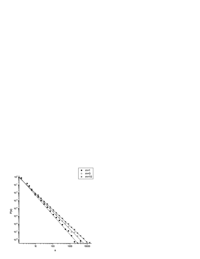
Figure 2: Results from a 250000 vertices simulation for model A for different values of $m$. On the left the strength distribution is compared with Eq.4. On the right the degree distribution is compared with Eq.8. Simulation results are points while lines represent the analytical results.

To check Eq.6 we integrated it for different values of $m$ and fixed $t$. This integral represents the number of occupied cells of the adjacency matrix and can be compared with results obtained by simulations. The results are shown in Fig.3. As we can see the uncorrelated approximation is very good for small values of $m$, but it fails to reproduce the behavior of the system for larger values of $m$, when correlations are stronger.

In Fig.2 we plot the simulations results against Eq.4 and Eq.8 for different values of $m$. In the case of the strength distribution the goodness of the fit is excellent, while in the case of the degree distribution the approximate result of Eq.8 gives just an approximate fit for large values of $m$, and it is because of the growing strength of correlations in the network for large values of $m$.

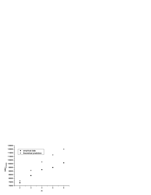
Figure 3: Comparison between the numerical integration of Eq.6 and numerical simulations. This integral represents the number of occupied cells of the adjacency matrix evaluated for $t=20000$ and varying values of $m$, while the empirical data count the effective number of occupied cells.

III Model B

In this section we build and analyze a multi-directed accelerated growing Eulerian network that is an accelerated version of the previous model and we will call it $ModelB$. In order to do this we replace the constant addition of $m$ edges at each time step with a number of edges $m^{\prime}$ that grows linearly with time, that is $m^{\prime}=\alpha t$. In this way at every time step we have an increasing number of edges added to the network. The obtained results and the used techniques are similar to the ones used in l1 . Nevertheless this extension of the previous model is designed to get closer to the topology of real language networks, as they display an accelerated evolution, and it is important for completeness in the discussion of the subject.

Keeping this in mind we can describe our modified model. We start with a chain of some connected vertices. At each time step we create a new vertex and $\alpha t+2$ new directed edges (Fig.1). In particular at each time step

a- The new vertex will acquire one in-link with the constraint the network must follow EC.

b- The remaining $\alpha t+1$ in-links will be attached to old vertices with a probability proportional to their in-strength with the constraint the network must follow EC.

The coefficient $\alpha$ will be chosen to fit with that found in real language networksap .

The equation for the strength evolution of the strength of vertex $i$ is

$$\frac{ds(t,t_{i})}{dt}=(\alpha t+1)\frac{s(t,t_{i}))}{\int_{0}^{t}dt_{i}s(t,t_{i})}.$$ (9)

The right hand side of the last equation takes into account that $\alpha t+1$ vertices can acquire a link with probability proportional to their normalized strength $\frac{s(t,t_{i})}{\int_{0}^{t}dt_{i}s(t,t_{i})}$. The integral at the denominator in the right hand side of Eq.9 represents the total strength of the network and is $\frac{1}{2}\alpha t^{2}+2t$.

Solving Eq.9 with initial condition $s(t_{i},t_{i})=1$ we obtain

$$s(t,t_{i})=\left(\frac{t}{t_{i}}\right)^{\frac{1}{2}}\left(\frac{\alpha t+4}{\alpha t_{i}+4}\right)^{\frac{3}{2}}.$$ (10)

To calculate the strength distribution we use the fact that

$$P(s,t)=-\frac{1}{t}(\frac{\partial s(t,t_{i})}{\partial t_{i}})^{-1}|_{t_{i}=s(t,t_{i})}$$ (11)

and we get

$$P(s,t)=\frac{2t_{i}}{ts}$$ (12)

where $t_{i}(s,t)$ is the solution of Eq.10.

This distribution has two regimes separated by a cross-over given approximatively by $s_{cross}\approx(\alpha t)^{\frac{1}{2}}(\frac{\alpha}{8}t+\frac{1}{2})^{\frac{3}{2}}$.

Below this point Eq.12 scales with a power law as

$$P(s)\propto s^{-\frac{3}{2}}$$ (13)

while, for $s>s_{cross}$,

$$P(s)\propto s^{-3}.$$ (14)

These results are well confirmed by numerical simulations as shown in Fig.4.

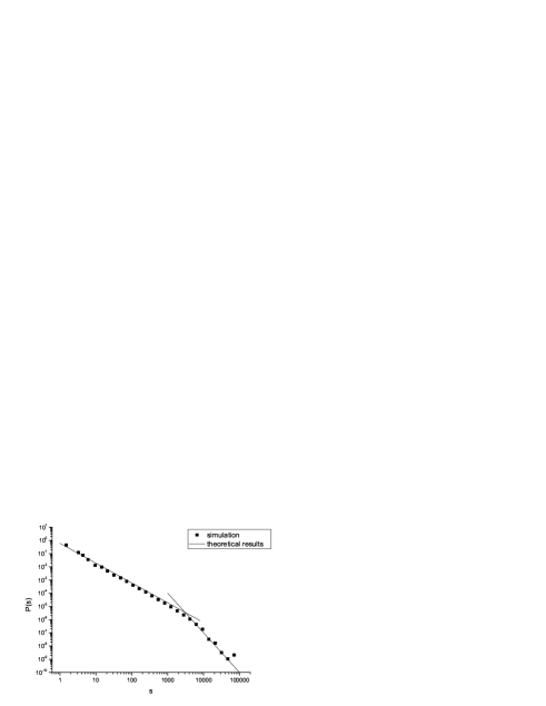
Figure 4: Comparison between the numerical simulation for model B in a network of 50000 vertices and Eq.13 and Eq.14.

IV Model C

To complete this work we introduce a non-Eulerian version of model A and we call it $ModelC$.

We start with $2m$ randomly connected vertices. At each time step we create a new vertex and $m+2$ new directed edges. In particular at each time step

a- The new vertex will acquire one in-link and one out-link.

b- The remaining $m+1$ out-links will be attached to old vertices with probability proportional to their out-strength.

c- The remaining $m+1$ in-links will be attached to old vertices with probability proportional to their out-strength.

For this model the same equations apply as with the Eulerian Model A with the same arguments, so that it displays equivalent topological properties, that is weight, strength and degree distributions. The main difference at this level of observation is that in the Eulerian case $s^{in}=s^{out}$ in an exact sense, while in this case this condition holds only on average.

V Conclusions

In this work we contextualize phenomena that manifest as a continuous chain of repeated elements in a novel way, within the framework of network theory. We show that such phenomena, such as human language, DNA chains, etc.., are described by Eulerian graphs. Eulerian graph topology ensures that every newly connected vertex of the network is connected to the last linked vertex. So we introduce and analyze different kinds of growing networks built to produce an Eulerian graph. We are able to find the main topological properties for this kind of network and we find that the resulting exponents for the strength and degree distributions are compatible with those of real networks. We then extend our model to a non-Eulerian one.

It is worth noting that, in the context of the standard network analysis, no striking differences emerge between the Eulerian network and its non-Eulerian counterpart. We performed a clustering coefficient analysis, but it was not worth showing it, since the differences between the average number of triangles formed in the network in the Eulerian and non-Eulerian case didn’t differ significatively. Even a Shannon entropy analysis wouldn’t define any relevant difference between the two different growing mechanisms, since it is based on the frequency of the elements more than on their structural organization. Considering this and the fact that the geometry of the two different networks are so dissimilar, dissimilar as a tree and a chain, we would like to emphasize the lack of statistical tools, in network theory, to characterize in a significant statistical way the different morphologies of different networks.

This work is mainly focused on the analysis of written human language, but it is also important for the study of directed and weighted growing networks. An important extension of these models, that could be taken into consideration for further investigations, is the growth of a network governed by local growing rules. We showed in a previous workap that local growing rules are important to reproduce interesting features of human language and must be taken into account to generate a syntax-like structure.

- (1) A.L. Barabasi, R. Albert, H. Jeong, Physica A 272, 173 (1999).
- (2) A. Barrat, M. Barthelemy, R. Pastor-Satorras, A. Vespignani, Proc. Natl. Acad. Sci. USA 101, 3747 (2004).
- (3) A. Barrat, M. Barthelemy, A. Vespignani, Phys. Rev. E 70, 066149 (2004).
- (4) G. Chartrand, L. Lesniak, Graphs & digraphs, Chapman & Hall, 1996.
- (5) S.N. Dorogovtsev, J.F.F. Mendes, A.N. Samukhin, Phys. Rev. Lett. 85, 4633 (2000).
- (6) S.N. Dorogovtsev, J.F.F. Mendes, Proc. Roy. Soc. London B 268, 2603 (2001).
- (7) R. Ferrer i Cancho, R.V. Sole, Proc. Roy. Soc. London B 268, 2261 (2001).
- (8) A.P. Masucci, G.J. Rodgers, Phys. Rev. E 74, 026102 (2006).
- (9) M.A. Montemurro, P.A. Pury, Fractals 10, 451 (2002).
- (10) P. Sen, Phys. A, 346, 139 (2005).
- (11) H.A. Simon, Biometrika 42, 425 (1955).
- (12) O.V. Usatenko, V.A. Yampol’skii, Phys. Rev. Lett. 90, 110601 (2003).
- (13) G.K. Zipf, Human Behaviour and the Principle of Least Effort, Addison-Wesley Press, 1949.
- (14) X. Yu, Z. Li, D. Zhang, F. Liang, X. Wang, X. Wu, J. Phys. A 39, 14343 (2006).
- (15) There is a large on-line bibliography on linguistic and cognitive networks at http://complex.ffn.ub.es/ ramon/linguistic_and_cognitive_networks.html