Abstract

A new mean field statistical mechanics model of two interacting groups of spins is introduced and the phase transition studied in terms of their relative size. A jump of the average magnetization is found for large values of the mutual interaction when the relative percentage of the two populations crosses a critical threshold. It is shown how the critical percentage depends on internal interactions and on the initial magnetizations. The model is interpreted as a prototype of resident-immigrant cultural interaction and conclusions from the social sciences perspectives are drawn.

1 Introduction

In the last few decades the statistical mechanics approach has seen an impressive expansion in fields as diverse as combinatorial optimization, finance, biology and others. Its success relies upon the fact that every problem of many interacting parts may be studied by its methods and techniques. Our plan in this work is to introduce a statistical mechanics model with the purpose of describing two homogeneous groups of individuals whose interaction is imitative within the same group but may be imitative or counter-imitative between different groups. Such a model may represent a first attempt toward the construction of a statistical mechanics theory of the phenomenon of cultural interchange. When two populations come in contact, like in the case of immigration but also in a more general context through the media, it is often seen how cultural traits are sometimes mixed, while some other times one of the two dominates and prevails on the other. Examples are found in linguistics, as well as in opinion forming dynamics ([1],[2],[3]). One interesting feature of those changes is that sometimes they appear to be smoothly varying with the relative proportions of the two groups, some other times the crossing of a critical value triggers a jump of the observed quantity [4]. What we are building here is the mean field theory of the two population problem i.e. we consider every individual interacting with every other with the same strength. In future works we plan to introduce a more realistic model by allowing randomness of the interaction strength like in the Sherrington-Kirkpatrick spin glass model ([5] [6]) and also a more structured network connection like, for instance, the one predicted by the small-world theory [7] [8]. We want to stress that, although our model is inspired by the Curie-Weiss theory of ferromagnetism, the problem we deal with here is quite different because we do not study the phase transition in terms of the temperature but in terms of the relative size of the two populations.

The dictionary we plan to follow is easily explained by saying that a cultural trait is considered for simplicity as a dichotomic variable $\sigma_{i}=\pm 1$. The interaction between particles is built up as a sum of pairwise interactions and plays the role of cultural interaction between two individuals $i$ and $j$ as described by a potential, or a cost function, which simply reflects the will to “agree” or “disagree” among the two. The two attitudes of imitation or counter-imitation lie on a well established socio-psychological background [9, 10, 11]; on the other hand they have also a robust mathematical-physical ground since they have been used to study many particles theory of ferromagnetic and anti-ferromagnetic interactions.

The problem we have addressed with the help of an equilibrium statistical mechanics model is to establish whether -in the case of two populations placed in contact- there may be a phase transition in the average cultural trait from one of the two original cultural traits to the other. If so, for which value of the relative percentage of the two populations it happens. Moreover, we want to establish how the critical size depends on the original parameters in order to predict or potentially avoid unwanted dramatic phenomena sometimes occurring in society.

The parameters describing our system are $m_{1}^{*}$ and $m_{2}^{*}$ i.e. the magnetizations of the two populations prior to their interaction which represent the two culture legacies, the couplings $J_{1,1}$, $J_{2,2}$ which measure the strength of the imitation within each group and $J_{1,2}$ which measure the strength of the imitation or counter-imitation among the two groups. The phase transition is tuned by the parameter $\alpha=N_{1}/N$ which counts the percentage of immigrants, $1-\alpha=N_{2}/N$ being the fraction of residents.

Our results, explained in detail in section 3, show that when the mutual interaction between the two groups $J_{1,2}$ is small enough the transition from the resident to the immigrant culture is smooth. But for large values of the interaction there is a critical value of the immigrant percentage $\alpha_{c}$ crossing which the system undergoes a sudden change from the resident to the foreign culture.

We find moreover that high values of the culture legacy favour both the emergence of the immigrant culture ($\alpha_{c}$ decreases with $m_{1}^{*}$) and the persistence of the local culture ($\alpha_{c}$ increases with $m_{2}^{*}$) as intuition would suggest. On the contrary, a high internal imitation (high coesion and low diversification) makes each culture weaker toward the other ($\alpha_{c}$ increases with $J_{1,1}$ and decreases with $J_{2,2}$). This last result is rather counter-intuitive but not surprising since in social sciences it is often seen how a diversified culture dominates an opinionated one. From a technical point of view the dependence of $\alpha_{c}$ on $J_{1,1}$ and $J_{2,2}$ is explained by the detailed balance between energy and entropy, the second being the leading term in those situations in which a phase transition occurs.

2 The Model

The model we introduce is defined by the Hamiltonian

$$H(\sigma)=-\frac{1}{2N}\sum_{i,j=1}^{N}J_{ij}\sigma_{i}\sigma_{j}-\sum_{i}h_{i}\sigma_{i}\;,$$ (2.1)

see [12] for some results on the model.

The symbol $\sigma_{i}$ represents the opinion of the $i^{th}$ individual of the total population, which can either take value $\sigma_{i}=+1$ or $\sigma_{i}=-1$. We consider only the case of symmetric matrices $J_{i,j}$. The general case can be easily reduced to the symmetric one by standard methods.

We divide the total population $I$ into a partition of 2 subsets $I_{1}\cup I_{2}=I$, of $N_{1}=|I_{1}|$ and $N_{2}=|I_{2}|$ with $N_{1}+N_{2}=N$. Given two individuals $\sigma_{i}$ and $\sigma_{j}$ , their mutual interaction parameter $J_{ij}$ depends on their respective subsets, as specified by the matrix

$$\begin{array}[]{ll}\\ N_{1}\left\{\begin{array}[]{ll}\\ \end{array}\right.\\ N_{2}\left\{\begin{array}[]{ll}\\ \\ \\ \end{array}\right.\end{array}\!\!\!\!\!\!\!\!\begin{array}[]{ll}\quad\overbrace{\qquad}^{\textrm{$N_{1}$}}\overbrace{\qquad\qquad}^{\textrm{$N_{2}$}}\\ \left(\begin{array}[]{c|ccc}\mathbf{J_{11}}&&\mathbf{J_{12}}\\ \hline\cr&&&\\ \mathbf{J_{12}}&&\mathbf{J_{22}}\\ &&&\\ \end{array}\right)\end{array}$$

The interacting system is therefore described by three degrees of freedom: $J_{11}$ and $J_{22}$ tune the interactions within each of the two subsets, and $J_{12}$ controls the interaction between two individuals belonging to different sets. We assume $J_{11}>0$ and $J_{22}>0$, whereas $J_{12}$ can be either positive or negative.

Analogously, the field $h_{i}$ takes two values $h_{1}$ and $h_{2}$, depending on the subset containing $\sigma_{i}$, as described by the following vector:

$$\begin{array}[]{ll}N_{1}\left\{\begin{array}[]{ll}\\ \end{array}\right.\\ N_{2}\left\{\begin{array}[]{ll}\\ \\ \\ \end{array}\right.\!\!\!\!\!\!\end{array}\!\!\!\!\!\!\left(\begin{array}[]{ccc|c}h_{1}\\ \hline\cr\\ h_{2}\\ \\ \end{array}\right)$$

By introducing the magnetization of a subset $I$ as

$$m_{I}(\sigma)\;=\;\frac{1}{|I|}\sum_{i\in I}\sigma_{i}$$

and indicating by $m_{1}$ and $m_{2}$ the magnetizations within the subsets $I_{1}$ and $I_{2}$ and by $\displaystyle{\alpha=\frac{N_{1}}{N}}$ the fraction of the first group on the whole, we may easily express the Hamiltonian per particle as

$$\frac{H(\sigma)}{N}=\!\!\!\! - \!\!\!\!\frac{1}{2}\left[J_{11}\alpha^{2}m_{1}^{2}\!+\!2J_{12}\alpha(1\!-\!\alpha)m_{1}m_{2}\!+\!J_{22}(1\!-\!\alpha)^{2}m_{2}^{2}\right]-h_{1}\alpha m_{1}-h_{2}(1-\alpha)m_{2}$$

In order to study the thermodynamical properties of the model it is interesting to observe that the Hamiltonian is left invariant by the action of a group of transformations. The group is described by $G=\mathbb{Z}_{2}\times\mathbb{Z}_{2}\times\mathbb{Z}_{2}$.

We can represent a point in our parameter space as $(\mathbf{m},\mathbf{J},\mathbf{h},\mathbf{\hat{\alpha}})$, where

$$\mathbf{m}=\left(\begin{array}[]{c}m_{1}\\ m_{2}\end{array}\right),\quad\mathbf{J}=\left(\begin{array}[]{cc}J_{11}&J_{12}\\ J_{12}&J_{22}\end{array}\right),\quad\mathbf{h}=\left(\begin{array}[]{c}h_{1}\\ h_{2}\end{array}\right),\quad\mathbf{\hat{\alpha}}=\left(\begin{array}[]{cc}\alpha&0\\ 0&1-\alpha\end{array}\right).$$

Therefore, given the limitations on the values of our parameters, the whole parameter space is given by $S=[-1,1]^{2}\times\mathbb{R}^{2}\times\mathbb{R}_{+}\times\mathbb{R}^{2}\times[0,1]$.

If we consider the representation of $G$ given by the $8$ matrices

$$\left(\begin{array}[]{cc}\epsilon_{1}&0\\ 0&\epsilon_{2}\end{array}\right),\quad\epsilon_{i}=+1\textrm{ or }-1\quad\textrm{ and }\quad\left(\begin{array}[]{cc}0&\eta_{1}\\ \eta_{2}&0\end{array}\right),\quad\eta_{i}=+1\textrm{ or }-1$$

we can consider the action of $G$ on $S$ as given by

$$\phi:G\times S\rightarrow S$$

where

$$\phi[\mathbf{M},(\mathbf{m},\mathbf{J},\mathbf{h},\mathbf{\hat{\alpha})}]=(\mathbf{M}\mathbf{m},\;\mathbf{M}\mathbf{J}\mathbf{M^{-1}},\;\mathbf{M}\mathbf{h},\;\mathbf{M}\mathbf{\hat{\alpha}}\mathbf{M^{-1}})$$

for every $\mathbf{x}\in S$ and $\mathbf{M}\in G$ and it’s straightforward to check that

$$H(\mathbf{x})=H(\phi(\mathbf{M},\,\mathbf{x})).$$

This can be easily done by writing the Hamiltonian per particle in vector notation as

$$\frac{H(\mathbf{m},\mathbf{J},\mathbf{h},\mathbf{\hat{\alpha})}}{N}=\!\!-\frac{1}{2}\langle\mathbf{\hat{\alpha}}\,\mathbf{m},\mathbf{J}\mathbf{\hat{\alpha}}\,\mathbf{m}\rangle-\langle\mathbf{h},\mathbf{\hat{\alpha}}\,\mathbf{m}\rangle.$$

In order to obtain the analytic solution of the proposed model we consider the Boltzmann-Gibbs measure of weight

$$p(\sigma)=\frac{e^{-H(\sigma)}}{\sum_{\sigma}e^{-H(\sigma)}}$$

and in particular we want to compute the average total magnetization per particle on that state

$$\langle m\rangle\;=\;\frac{1}{N}\frac{\sum_{\sigma}\sum_{i}\sigma_{i}e^{-H(\sigma)}}{\sum_{\sigma}e^{-H(\sigma)}}\;.$$

For that purpose, it is useful to compute the pressure

$$P\;=\;\frac{1}{N}\log\sum_{\sigma}e^{-H(\sigma)}\;.$$

One can show (see [13]) that in the thermodynamical limit ($N\to\infty$) the pressure can be expressed as:

$$P=\sup_{\mu_{1},\mu_{2}}f(\mu_{1},\mu_{2}),$$ (2.2)

where

$$f(\mu_{1},\mu_{2}) = \frac{1}{2}\bigg{(}J_{11}\alpha^{2}\mu_{1}^{2}+J_{22}(1-\alpha)^{2}\mu_{2}^{2}+2J_{12}\alpha(1-\alpha)\mu_{1}\mu_{2}\bigg{)}+$$ (2.3)

$$+\ \alpha h_{1}\mu_{1}+(1-\alpha)h_{2}\mu_{2}+$$

$$+\ \alpha\left(-\frac{1+\mu_{1}}{2}\ln\left(\frac{1+\mu_{1}}{2}\right)-\frac{1-\mu_{1}}{2}\ln\left(\frac{1-\mu_{1}}{2}\right)\right)+$$

$$+\ (1-\alpha)\left(-\frac{1+\mu_{2}}{2}\ln\left(\frac{1+\mu_{2}}{2}\right)-\frac{1-\mu_{2}}{2}\ln\left(\frac{1-\mu_{2}}{2}\right)\right)\ .$$

The first two lines represent the internal energy contribution and the second the entropy in a state of magnetization ${\bf\mu}=(\mu_{1},\mu_{2})$.

Once we have the pressure it’s easy to show that $\langle m\rangle$, in the thermodynamical limit, can be written as

$$\langle m\rangle=\alpha\langle m_{1}\rangle+(1-\alpha)\langle m_{2}\rangle$$ (2.4)

where $\langle m_{1}\rangle$ and $\langle m_{2}\rangle$ (the average magnetizations within the subsets $I_{1}$ and $I_{2}$) are found to be the maximizers of $f(\mu_{1},\mu_{2})$ in (2.2).

The stationarity condition for the function $f(\mu_{1},\mu_{2})$ in (2.2) gives

$$\left\{\begin{array}[]{lll}\mu_{1}&=&\tanh(J_{11}\alpha\mu_{1}+J_{12}(1-\alpha)\mu_{2}+h_{1})\\ \mu_{2}&=&\tanh(J_{12}\alpha\mu_{1}+J_{22}(1-\alpha)\mu_{2}+h_{2})\\ \end{array}\right.$$ (2.7)

This system has generically nine solutions, four of which are stable solutions corresponding to relative maxima. These can be found numerically by interpreting the (2.7) as a fixed point equation of a two dimensional map. Similar physical systems do appear in the litterature in the study of metamagnets (see [15] and [14]) but they only deal with a simplyfied subcase of the (2.7) which correspond to search the solutions on a submanifold of the entire phase space. Moreover the way the magnetic fields are coupled to the pre-interaction magnetizations is completely unusual and unprecedented in physics. See also [16] for the use of the mean field ferromagnetic equations for a single population.

In our model the values of $h_{1}$ and $h_{2}$ shall not be considered as independent parameters but as functions of the average magnetizations and internal interactions in each original population when there is no mutual interaction between the two.

Denoting by $m^{*}_{1}$ and $m^{*}_{2}$ the magnetization values at equilibrium within the population 1 and 2 respectively, one has:

$$\left\{\begin{array}[]{c}h_{1}=\tanh^{-1}(m^{*}_{1})-J_{1,1}m^{*}_{1}\\ h_{2}=\tanh^{-1}(m^{*}_{2})-J_{2,2}m^{*}_{2}\end{array}\right.$$ (2.10)

So our main quantity $\langle m\rangle$ is a function of five parameters:

$$\langle m\rangle=\langle m\rangle(\alpha,J_{11},J_{22},J_{12},m^{*}_{1},m^{*}_{2})\ .$$ (2.11)

3 Numerical results

We have analyzed the numerical solutions of the system (2.7) and studied the behaviour in terms of the free parameters.

The main quantity we study is $\langle m\rangle$. In the sociological context it may represent the average opinion of the interacting system consisting of the population of immigrants and residents.

In particular, two main questions are addressed. First, what are the conditions that may lead to an instability of $\langle m\rangle$ in terms of the fraction of immigrants $\alpha$? Second, how does the critical behaviour depends on the free parameters?

As discussed in the previous section we may restrict our study to the case of $J_{1,2}\geq 0$. The behaviour in the other regime can be deduced by symmetry.

The results can be summarised in the following way.

Figure 1: $\langle m\rangle$ as a function of $J_{1,2}$ and $\alpha$

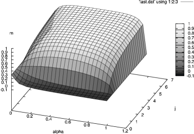
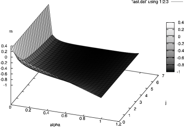
Figure 1 shows the total average magnetization $\langle m\rangle$ as a function of $\alpha$ and the mutual interaction strength $J_{1,2}$.

What we see is that when $J_{1,2}$ is small enough the magnetization is smoothly varying in $\alpha$ from $m^{*}_{2}$ to $m^{*}_{1}$ i.e. the value of the magnetization within the residents and immigrants before the mutual interaction takes place. But when the $J_{1,2}$ crosses a critical value we observe that the magnetization exhibits a discontinuous transition. The value of $\alpha$ at which the discontinuity occurs does not depend on $J_{1,2}$. This means that the critical $\alpha_{c}$ depends on the four parameters $J_{1,1},J_{2,2},m^{*}_{2},m^{*}_{1}$. Numerical results show that $\alpha_{c}$ can be arbitrarily small for a suitable choice of the parameters it depends on. It is interesting then to investigate how $\alpha_{c}$ depends on the interactions and on the original values of the magnetizations.

We first present the results concerning the dependence of $\langle m\rangle$ in terms of the original magnetization within populations 1 and 2, i.e. the opinion of the immigrants and residents before interaction. In order to do so we study the following interaction matrix for $j\in[0,7]$

$$\mathbf{J}=\left(\begin{array}[]{cc}1\quad j\\[10.0pt] j\quad 1\end{array}\right)$$ (3.12)

where $J_{11}=J_{22}=1$ and $J_{12}=j>0$. We work with $\alpha\in[0,1]$, and study $\langle m\rangle$ w.r.t. $\mathbf{m^{*}}=(m^{*}_{1},m^{*}_{2})$.

The dependence of $\alpha_{c}$ in terms of the cultural legacies $\mathbf{m^{*}}$ appears to be rather intuitive: the more the immigrant population is polarised (large negative values of $m_{1}^{*}$), the less is the amount of immigrants necessary to induce a phase transition. Equivalently, the more the resident population is polarised (large positive value of $m_{2}^{*}$ ) the larger is $\alpha_{c}$.

Figure 2: Magnetization surface when (a) $\mathbf{m}^{*}=(-0.05,0.3)$; (b) $\mathbf{m}^{*}=(-0.2,0.3)$; (c) $\mathbf{m}^{*}=(-0.3,0.3)$; (d) $\mathbf{m}^{*}=(-0.5,0.3)$; (e) $\mathbf{m}^{*}=(-0.95,0.3)$; (f) bottom graph: $\mathbf{m}^{*}=(-0.3,-0.9)$; top graph: $\mathbf{m}^{*}=(0.3,0.9)$.

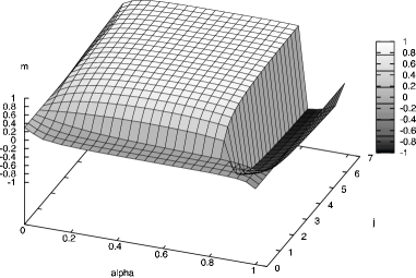
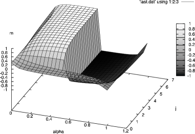
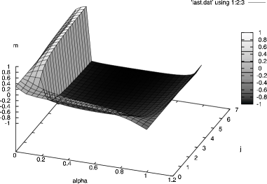
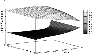
Pictures (a)-(f) in Figure 2 show some cases of surface $M_{\mathbf{m^{*}}}(j,\alpha)$ for $m^{*}_{2}=0.3$ and several $m^{*}_{1}$. The values of $\alpha_{c}$ increase from 0 to 1 when $m^{*}_{1}$ varies from -0.05 to -0.95 (pictures (a) to (e)), while there is no abrupt transition when both $m^{*}_{1}$ and $m^{*}_{2}$ are positive (picture (f), top). The surface is symmetrical when taking both $m^{*}_{1}$ and $m^{*}_{2}$ negative (picture (f), bottom).

Socially speaking, the transition has to be read as follows: for large enough intercultural interactions $j$, when $\alpha<\alpha_{c}$ the resident culture prevails, while when $\alpha>\alpha_{c}$ the immigrant culture prevails. An abrupt switch occurs when $\alpha=\alpha_{c}$. Consequently, the critical value shows what fraction of immigrants is necessary to make the resident opinion lose its leadership over the entire population.

The value of $\alpha_{c}$ varies with $\mathbf{m^{*}}$. We may build a surface ${\cal S}_{\alpha_{c}}$ (Figure 3) where $\alpha_{c}$ is a function of the non-interacting configuration $\mathbf{m}^{*}$ with $m^{*}_{1}\in[-1,0]$ and $m^{*}_{2}\in[0,1]$. We may notice that $\alpha_{c}=\frac{1}{2}$ when $m^{*}_{1}=-m^{*}_{2}$ and the surface has the symmetry: $\alpha_{c}(m^{*}_{1},m^{*}_{2})=1-\alpha_{c}(-m^{*}_{2},-m^{*}_{1})$. The value of $\alpha_{c}$ is almost constant $\alpha_{c}=0$ when $\mathbf{m}^{*}\in T_{1}=\{-1\leq m^{*}_{1}\leq-\frac{1}{2}\ ,0\leq m^{*}_{2}\leq-\frac{1}{2}-m^{*}_{1}\}$. Due to the symmetry, $\alpha_{c}=1$ when $\mathbf{m}^{*}\in T_{2}=\{-\frac{1}{2}\leq m^{*}_{1}\leq 0\ ,\ \frac{1}{2}\leq m^{*}_{2}\leq\frac{1}{2}-m^{*}_{1}\}$.

Figure 3: The transition value $\alpha_{c}$ for the ferromagnetic model as a function of the non-interacting configuration $(m^{*}_{1},m^{*}_{2})$ with $m^{*}_{1}\in[-1,0]$ and $m^{*}_{2}\in[0,1]$.

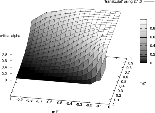
The $\alpha$-critical surface ${\cal S}_{\alpha_{c}}$ shows what is the amount of immigrants necessary to have a change, given the initial cultures of the two non-interacting populations. Its behaviour agrees with intuition: the stronger the immigrant original culture, the smaller the percentage of them necessary to lead the opinion i.e. the critical percentage decreases with the immigrant culture strength. Viceversa the percentage increases with a stronger resident culture.

We shall now investigate the dependence of $\alpha_{c}$ on $J_{1,1}$ and $J_{2,2}$. To do this we start from Figure 1 and increase $J_{1,1}$ from 0.9 to 1.05, leaving the other parameters unchanged.

Figure 4: Magnetization surfaces (a) before and (b) after increasing the immigrant population’s interaction parameter $J_{11}$. (c) $\alpha_{c}$ strictly increases with $J_{11}$.

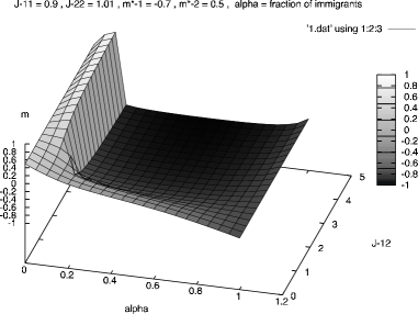
The result of this variation is Figure 4: comparing it with the original picture, shown on the side, we see how the discontinuity in the surface has been drawn forward to a bigger value of $\alpha_{c}$: the critical percentage turns out to be increasing with the strength of the immigrant interaction $J_{1,1}$. The more the immigrants tend to imitate each other, the less effective their influence is in the interacting system. This result may seem at odds with intuition, and suggests that a more diversified population is more likely to impose its cultural traits.

This turns out to be a general feature of our simulations. Consider Figure 4: we have set $J_{1,2}=2$ and we have let $J_{11}$ vary between 0 and 1.2. As a result, we see how $\alpha_{c}$ increases monotonically with $J_{11}$.

Similarly, by symmetry considerations, it is straightforward that an increase in the interaction strength within population 2 ($J_{22}$) will lead to a decrease in $\alpha_{c}$.

Figure 5: $\alpha_{c}$ as a function of $J_{1,1}$ and $J_{2,2}$

As a consequence, our study of the model reveals that an increase in the interaction strength within a population doesn’t reinforce the population’s own position within the total magnetization but, on the contrary, hastens the discontinuous transition towards the competing population’s culture. The dependence of $\alpha_{c}$ on $J_{11}$ and $J_{22}$ is summarised by Figure 5.

4 Comments

In this paper we have analyzed a two population mean field statistical mechanics spin model. The study of its phase structure in terms of the relative proportions of the two populations has been carried on. We have seen that the average magnetization of the two interacting populations may vary smoothly when the interchange coefficient is small, but also abruptly when the coefficient is large. The critical value of the relative proportion has been studied in terms of both the initial values of the magnetizations within each population and a standard behaviour has been found. More intriguing is the observed dependence of the critical percentage in terms of the internal cohesion of each group. Due to a fine balance between internal energy and entropy we find that a strong cohesion penalizes the group.

The model proposed is the simplest statistical mechanics model for the phenomenon of cultural contact, especially in the case of the residents and immigrants interaction. The dictionary associates a dichotomic opinion (like being in favour or against death penalty) to the two values of the spins. The interaction between two individuals is mapped into a ferromagnetic term in the Hamiltonian. The mean values within residents and immigrants of the country opinions are considered as cultural legacies and are compared to the average of the interacting mixed populations. The main result of this work from the social science perspective is to show that statistical mechanics predicts the possibility to have cultural dramatic changes during social contact. Moreover, it shows that the resident culture is more stable in its ability to survive the immigrant influence when imitation between residents is low and diversification is high. Equivalently, the power of the immigrant culture to take over and spread into the new country is lowered by a high internal imitation and low diversification.

From the mathematics and physics point of view our model generalizes the theory of the metamagnets introduced in [14] and [15]. The presence of extra degrees of freedom, in particular the pre-interaction magnetizations, in the two dimensional map makes our system difficult to study even though we may express the solution in a variational form like in the mean field theories: for instance it is not known yet what is the analytical condition needed to ensure the phase transition nor a detailed knowledge of its nature. Even simplified cases in which the solution is searched in submanifold of the entire phase space are not exactly solvable in a rigorous mathematical sense (see [17]); we will return on the rigorous results available in a future contribution [13].

Acknowledgments: we thank C. Giardinà and S.Ghirlanda for useful discussions.

References

- [1] Ben-Naim E., Redner S., Krapivsky P.L., Bifurcation and patterns in compromise processes, Physica D, 183: 190-204, 2003.
- [2] Friedkin N.E., Johnson E.C., Social influence and opinion, J. Math.Sociol., 28:193-205, 1990.
- [3] Weisbuch G., Deffuant G., Amblard F., Nadal J.-P., Meet, Discuss and Segregate!, Complexity, 7, 3: 55-63, 2002.
- [4] Q. Michard, J.-P. Bouchaud, Theory of collective opinion shifts: from smooth trends to abrupt swings, cond-mat/0504079, to appear in Quality and Quantity
- [5] D.Sherrington, S.Kirkpatrick, Solvable Model of a Spin Glass Phys. Rev. Lett., 35, 1975
- [6] Mezard, Parisi, Virasoro, Spin Glass Theory and Beyond, World Scientific, 1987
- [7] Watts D.J. and Strogatz S., Collective dynamics of ‘small-world’ networks, Nature, 394: 440, 1998
- [8] Klemm K., Eguiluz V.M., Toral R., San Miguel M., Nonequilibrium transitions in complex networks: A model of social interaction, Phys. Rev. E 67: 026120.1-026120., 2003
- [9] Bond R., Smith P. B., Culture and conformity: A meta-analysis of studies using Asch s (1952b,1956) line judgment task, Psychological Bulletin: 119, 111-137, 1996
- [10] Michinov E. and Monteil J.M., The similarity-attraction relationship revisited: divergence between affective and behavioral facets of attraction, European Journal of Social Psychology, 32: 485-500, 2002
- [11] Byrne D., An overview (and underview) of research and theory within the attraction paradigm, Journal of Personality and Social Psychology, 14: 417-431, 1997
- [12] Contucci P., Ghirlanda S., Modeling society with statistical mechanics: an application to cultural contact and immigration, physics/0606062, to appear in Quality and Quantity, 2006
- [13] Contucci P., Gallo I., In preparation
- [14] Kincaid J.M., Cohen E.G.D., Phase diagrams of liquid helium mixtures and metamagnets: experiment and mean field theory, Physics Letters C, 22: 58-142, 1975
- [15] Galam S., Yokoi C. S. O., Salinas S. R., Metamagnets in uniform and random fields, Phys. Rev. B, 57: 8370-8374, 1998
- [16] Durlauf S. N., How can statistical mechanics contribute to social science?, Proc Natl Acad Sci U S A , 96: 10582-10584, 1999
- [17] Kulske C., Le Ny A., Spin-Flip Dynamics of the Curie-Weiss Model: Loss of Gibbsianness with Possibly Broken Symmetry, Communications in Mathematical Physics, 271: 431-454, 2007