A Zeeman Slower based on magnetic dipoles

Abstract

A transverse Zeeman slower composed of an array of compact discrete neodymium magnets is considered. A simple and precise model of such a slower based on magnetic dipoles is developed. The theory of a general Zeeman slower is modified to include spatial nonuniformity of the slowing laser beam intensity due to its convergence and absorption by slowed atoms. The slower needs no high currents or water cooling and the spatial distribution of its magnetic field can be adjusted. In addition the slower provides a possibility to cool the slowed atoms transversally along the whole length of the slower. Such a slower would be ideal for transportable optical atomic clocks and their future applications in space physics.

I Introduction

The sources of slow atoms based on laser cooling of their translation degree of freedom are widely used in many modern atomic physics experiments. At the present time a Zeeman slower Phillips is the most efficient slower of that type. Recently a maximal flux of cold Rb atoms as high as $3.2\times 10^{12}\,$at/s, produced by a Zeeman slower with an additional section for the transverse laser cooling of atoms, has been demonstrated Slowe . For some alkali atoms like Rb and Cs a Zeeman slower can be substituted with more compact sources based on magneto-optical traps Riis ; Dieckmann ; Ovchinnikov , the typical flux of which is between $10^{9}$ and $10^{10}\,$at/s. The most intense source of that type based on two-dimensional magneto-optical trap is able to produce the flux of $6\times 10^{10}\,$at/s Schoser . On the other hand, for many other atoms and experimental conditions a Zeeman slower is the only choice. A standard Zeeman slower uses a special current-carrying coil to create a proper spatial distribution of the magnetic field along its axis, the purpose of which is to compensate a Doppler shift of the decelerated atoms with a corresponding Zeeman shift.

An advantage of a Zeeman slower based on permanent magnets is that it does not need high currents and corresponding cooling of its coils. The existent approach to such a permanent Zeeman slower consists in substitution of standard Zeeman coils with analogous ring-like magnets made of plastic-bonded permanent magnets Adler , which can be machined to any form prior their magnetization. The disadvantage of these magnets is that they are not as strong as dense magnets and their strength is subject to fluctuations due to the inconsistancy of the density of the magnetic material.

In this paper it is proposed to use an array of small neodymium magnets to create a required magnetic field distribution of a Zeeman slower. A simple model of the slower, based on point-like magnetic dipoles is introduced. It is shown that this model works well even for magnets of a size comparable to their distance from the axis of the slower. The design of such a slower includes a possibility to vary the distances of the individual magnets from the axis of the slower, which allows fine tuning of the magnetic field.

In the first part of the paper the existent standard theory of a Zeeman slower is extended to apply it to a cooling laser beam with a nonuniform distribution of its intensity along the axis of the slower. It is shown how the absorption of the cooling light can be included in calculation of the most optimal spatial distribution of the magnetic field of the slower. It is proposed in the case of a nonuniform laser field to use instead of a standard design parameter $\eta$ a slightly different parameter $\epsilon$, which relates the designed local deceleration of atoms to its maximum possible value at the same location at given laser intensity. It is shown that the most optimal cooling of the decelerated atoms takes place at $\epsilon=0.75$.

In the first section a numerical approach to the calculation of the optimal spatial distribution of the magnetic field of a Zeeman slower is described for a general case of a cooling laser beam with non-uniform intensity distribution. In the second section Zeeman slowers based on permanent magnetic dipoles are discussed. In the outlook section the construction of a transverse Zeeman slower based on neodymium magnets and its applications are discussed. Finally, in the conclusion the main results are summarized.

II General theory of Zeeman slower

In a Zeeman slower atoms are decelerated in a counterpropagating resonant laser beam due to momentum transfer from spontaneously scattered photons. An existent analytical theory of a Zeeman slower Napolitano ; Metcalf is based on uniform deceleration of atoms in a field of a laser beam with uniform intensity distribution. In practice intensity of the slowing laser beam is never uniform. There are several reasons for that. First, to increase an overlap of the laser beam with the expanding atomic beam and to provide some additional transverse cooling of the decelerated atoms, convergent laser beam is usually used. Second, absorption of laser light by slowed atoms essentially changes the distribution of intensity of light along the axis of a Zeeman slower.

Below a procedure of numerical calculation of the magnetic field distribution of a Zeeman slower is described for a general case of a slowing laser beam with non-uniform spatial distribution of its intensity. To keep it simple, dependence of the light intensity along only one of the coordinates z, which is the axis of a Zeeman slower, is considered.

The spontaneous light pressure force is given by

$$F(v,z)=\frac{\hbar k\Gamma}{2}\frac{s_{0}(z)}{1+s_{0}(z)+4[\delta_{0}+kv-\mu^{\prime}B(z)/\hbar]^{2}/\Gamma^{2}},$$ (1)

where $k$ is the wave vector of light, $s_{0}(z)$ is the local on-resonance saturation parameter of the atomic transition, $\Gamma$ is the linewidth of the transition, $\delta_{0}$ is the laser frequency detuning, $v$ is the velocity of the atom, $\mu^{\prime}$ is the magnetic moment for the atomic transition and $B(z)$ is the local magnitude of the magnetic field. The velocity dependence of the force is determined by the effective frequency detuning $\Delta_{eff}=\delta_{0}+kv-\mu^{\prime}B(z)/\hbar$, which includes the Doppler shift $kv$ of the atomic frequency. The maximum value of the local deceleration, provided by the force, is achieved at exact resonance, when $\Delta_{eff}=0$, and is given by

$$a_{max}(z)=\frac{\hbar k\Gamma}{2m}\frac{s_{0}(z)}{1+s_{0}(z)},$$ (2)

where m is the mass of the atom. Although the maximum deceleration can be used to estimate the shortest possible length of a Zeeman slower, this can not be realised in practice. At exact resonance an equilibrium between the inertial force of the decelerated atoms and the light force is unstable and any slight increase of the atomic velocity due to imperfection of the magnetic field distribution or spontaneous heating of atoms will lead to decrease of the decelerating force and subsequent loss of atoms from the deceleration process. In practice the deceleration of atoms is realized at a fraction of the maximum deceleration

$$a(z)=\epsilon a_{max}(z),$$ (3)

where $\epsilon<1$. Note that the coefficient $\epsilon$ in our case corresponds to the ratio between the reduced local acceleration and the maximum possible acceleration at the same location, which is a function of the local saturation parameter $s_{0}(z)$. In a standard treatment Napolitano ; Metcalf a similar coefficient $\eta$ appears, which relates the actual deceleration to the maximum possible deceleration at infinite intensity of laser light. When the deceleration is less than $a_{max}$ the decelerated atoms stay on the low-velocity wing of the Lorentzian velocity profile of the light force (1) and andergo stable deceleration. The corresponding equilibrium velocity $v(z)$ of the decelerated atoms, which is less than the resonant velocity $v_{res}(z)=(\mu^{\prime}B(z)/\hbar-\delta_{0})/k$, is determined by

$$kv(z)=kv_{res}(z)-\frac{\Gamma}{2}\sqrt{(1+s_{0}(z))\frac{1-\epsilon}{\epsilon}}.$$ (4)

The most optimal offset of the equilibrium velocity $v(z)$ from the resonant velocity $v_{res}(z)$ is achieved at a point where the derivative of the force (1) reaches its maximum, because the damping of the relative motion of atoms around this point is maximal. It is easy to show that within our definition of the $\epsilon$ coefficient (3) this most optimal cooling condition is achieved exactly at $\epsilon=0.75$. The damping coefficient of the force decreases with the increas of the intensity of the laser field. Therefore, choosing of the most optimal intensity of the cooling beam for a Zeeman slower is a compromise between having a large deceleleration force and low velocity spread of the decelerated atoms. Usually the saturation parameter of a Zeeman slower is chosen to be about 1.

The procedure of calculation of the spatial distribution of a Zeeman slower looks as follows. First, the actual velocity of the slowing atoms is calculated numerically according to the formula

$$\frac{dv(z)}{dz}=\epsilon\frac{\hbar k\Gamma}{2m}\frac{s_{0}(z)}{1+s_{0}(z)},$$ (5)

After that the resonant velocity can be determined from the eq. (4) and the corresponding distribution of the magnetic field calculated as

$$B(z)=\hbar(\delta_{0}+kv_{res}(z))/\mu^{\prime}.$$ (6)

The distribution of the saturation parameter $s_{0}(z)$ on the axis of the slower has to be taken according to the convergence of the cooling laser beam and its absorption by the slowed atoms. If the influence of the convergence of the laser beam to the spatial distribution of the saturation parameter is easy to include, but the calculation of the absorption of light by the decelerated atoms is not so straightforward. The problem of the propagation of atoms and light through each other while they are mutually interacting is difficult to solve. On the other hand, it can be easily solved by inverting the direction of motion of the atoms and calculating their acceleration along the laser beam, starting from the end edge of a Zeeman slower. For atoms copropagating with the laser beam, the change of the atomic velocity, which is responsible for the local density of atoms, and the change of the intensity of light at each point inside the slower can be simultaneously computed from their values at the preceding spatial step. The corresponding distribution of the saturation parameter along the Zeeman slower can be found from the equation

$$\frac{ds_{0}(z^{\ast})}{dz^{\ast}}=-s_{0}(z^{\ast})n(z^{\ast})\frac{\sigma_{0}\epsilon}{1+s_{0}(z^{\ast})}+s_{0}(z^{\ast})\frac{2}{l_{0}-z^{\ast}},$$ (7)

where $z^{\ast}=z_{f}-z$ is a coordinate along the direction of propagation of the laser beam, which starts at the end point $z=z_{f}$ of the Zeeman slower, $n(z^{\ast})$ is the local density of atoms, $\sigma_{0}$ is the resonant light scattering cross section and $l_{0}$ is the distance from the end edge of the slower to the waist of the converged laser beam. The first term in the right side of the equation is responsible for the absorption of light and the second one for the convergence of the laser beam. It is supposed that the focal plane of the laser beam is located outside the slower, such as $l_{0}$ is larger than its length. In this one-dimensional problem the density means the number of atoms per unit length along the $z$-axis of the slower. The local density of the slowed atoms at $z^{\ast}$ is given by

$$n(z^{\ast})=\frac{A}{v(z^{\ast})}\int_{v(z^{\ast})}^{v_{0}}\Phi(v_{z},u)dv_{z},$$ (8)

where $\Phi(v_{z},u)=0.5(v_{z}^{3}/u^{4})\exp(-0.5v_{z}^{2}/u^{2})$ is the flux density in the initial thermal atomic beam, $u=\sqrt{k_{B}T/m}$, $v_{0}$ is the capture velocity of the slower and $A$ is a coefficient to normalize the density to the total flux of atoms. In this formula the density of atoms at the location $z^{\ast}$ is determined by the integrated flux of atoms between the velocities $v(z^{\ast})$ and $v_{0}$, which is divided by the local velocity of the slowed atoms $v(z^{\ast})$. The analytical solution of the eq. (8) is given by

$$n(z^{\ast})=A\frac{(2u^{2}+v(z^{\ast})^{2})e^{-\frac{v(z^{\ast})^{2}}{2u^{2}}}-(2u^{2}+v_{0}^{2})e^{-\frac{v_{0}^{2}}{2u^{2}}}}{2u^{2}v(z^{\ast})}.$$ (9)

This function predicts rapid increase of the density of the slowed atoms towards the end of the slower, where the velocity $v(z^{\ast})$ becomes small, which was confirmed experimentally in Firmino ; Napolitano by direct measurement of the fluorescence of atoms inside a Zeeman slower.

As an example we will consider here a Zeeman slower for Sr atoms similar to one in Lemonde , where the ${}^{1}S_{0}\rightarrow^{1}P_{1}$ transition of Sr with wavelength $\lambda=461\,$nm and natural linewidth $\Gamma=2\pi\times 32\,$MHz is used for cooling of the translation motion of atoms. The slower is designed to slow atoms from the initial velocity $v_{0}=420\,$m/s down to the final velocity $25\,$m/s over a distance $L_{s}=25\,$cm with the efficiency parameter $\epsilon=0.6$. The value of the $\epsilon$ parameter was chosen to be below its optimal value $\epsilon=0.75$ to include possible imperfection of the magnetic field distribution of the slower. The thermal velocity of the initial atomic beam is taken to be $u=292\,$m/s, which corresponds to the temperature of $T=630\,^{\circ}$C. For the given capture velocity of the slower, the flux of the slowed atoms is about 28% of the total initial flux of thermal atoms. The cooling laser beam is taken to be convergent, such that its diameter at the output of the slower ($z=z_{f}=25\,$cm) is $d_{0}=1\,$cm and at its input ($z=0$) $d_{1}=0.3\,$cm. This corresponds to the distance between the output end of the slower and the waist of the laser beam of $l_{0}=L_{s}D_{0}/(d_{0}-d_{1})=35.7\,$cm. The saturation parameter at the end edge of the slower is set to be $s_{0}(z_{f})=1$. The total absorption of the cooling light in the slower was set to 50% of the total light power of the laser beam. Taking into account that each decelerated atom absorbs in average about 22000 photons it is easy to derive that absorption of 22.5 mW of laser power gives the total flux of cold atoms about $2.4\times 10^{12}\,$at/s, which corresponds to the total initial flux of the thermal atoms of $8.7\times 10^{12}\,$at/s. It is assured here that there are no losses of the atoms during their deceleration and extraction from the slower.

Figure 1: Spatial dependence of saturation parameter inside Zeeman slower in presence of 50% absorption (solid line) and without any absorption (dashed line).

Figure 1 shows the calculated spatial distribution of the saturation parameter of the atomic transition along the $z$-axis of the slower. The solid curve shows that the large absorption of the slowing light at the end of Zeeman slower, where the density of the slowed atoms reaches its maximum, leads to slight decrease of the saturation parameter, which can not be compensated by the convergence of the laser beam. The dashed curve corresponds to the case of absence of any absorption of the cooling light. Here the smaller initial saturation parameter $s_{0}(z_{f})=0.58$ is used to keep the capture velocity of the slower $v_{0}=420\,$m/s the same. In the absence of absorption the saturation parameter is growing monotonically due to convergence of the laser beam. Comparison of the derivatives of these curves shows that the absorption takes place mostly in the end half of the Zeeman slower, which is explained by higher density of atoms and lower saturation parameter at this part of the slower.

Figure 2: Spatial distribution of magnetic field inside Zeeman slower in presence of 50% absorption and convergent laser beam (solid line); for convergent laser beam and no absorption (dashed line); collimated laser beam and no absorption (dotted line).

Figure 2 shows the optimal spatial distribution of the magnetic field along the Zeeman slower, calculated from the formulas (1-8). The solid curve corresponds to the 50% absorption of the laser beam and the other parameters as above. The dashed curve shows the case, when the absorption is absent and the initial saturation parameter $s_{0}(z_{f})=0.58$. The dotted curve corresponds to a uniform deceleration of atoms in a laser beam of constant diameter and constant saturation parameter $s_{0}(z)=1.5$ in absence of absorption.

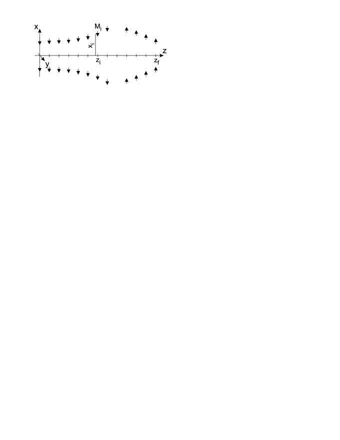
Figure 3: Schematic structure of Zeeman slower based on magnetic dipoles.

III Zeeman slower based on magnetic dipoles

It is proposed to use a Zeeman slower based on a quasiperiodic array of small permanent magnets as is shown in fig. 3. These magnets can be modeled as point-like magnetic dipoles (MD). There are two different possible configurations of such a slower, the transverse, when the dipoles are oriented perpendicularly to the axis of the slower (as in fig. 3) or the longitudinal one, when the dipoles are oriented along the axis and the resulted magnetic field of the slower is also directed along that axis.

To understand the basic difference between the two configurations, the field of a single magnetic dipole has to be considered first. For a magnetic dipole placed at the origin of a Cartesian system of coordinates and oriented along the x-axis, its magnetic field is described by the formulas

$$B_{x}=\frac{\mu_{0}M}{4\pi}\left[\frac{2x^{2}-y^{2}-z^{2}}{r^{5}}\right]$$

$$B_{y}=\frac{\mu_{0}M}{4\pi}\left[\frac{3xy}{r^{5}}\right]$$

$$B_{z}=\frac{\mu_{0}M}{4\pi}\left[\frac{3xz}{r^{5}}\right],$$ (10)

where $r=\sqrt{x^{2}+y^{2}+z^{2}}$ and $M$ is the magnetic moment of the dipole. Let us consider now a distribution of the magnetic field along the $z$-axis for a single MD placed at $x=R,y=0,z=0$, while it is oriented perpendicular or parallel to the $z$-axis. The corresponding distributions of the proper components of magnetic field are given by

$$B_{x}(z)=\frac{\mu_{0}M}{4\pi}\left[\frac{2R^{2}-z^{2}}{(R^{2}+z^{2})^{5/2}}\right]$$

$$B_{z}(z)=\frac{\mu_{0}M}{4\pi}\left[\frac{2z^{2}-R^{2}}{(R^{2}+z^{2})^{5/2}}\right].$$ (11)

For a symmetric distribution of the magnetic dipoles around the $z$-axis, all other components of the magnetic field at this axis are equal to zero. Figure 4 shows the corresponding distributions of $B_{x}(z)$ (solid line) and $B_{z}(z)$ (dashed line) for a MD with magnetic moment $M=1.86\,$Am² and $R=3\,$cm.

Figure 4: Spatial distribution of magnetic field of a point-like magnetic dipole. The distribution along the $z$-axis for a magnetic dipole oriented perpendicularly to the axis (solid line). The distribution for a dipole moment oriented parallel to the $z$-axis (dashed line).

For the perpendicular orientation of the MD, its field along the $z$-axis is mostly of the same sign, while for the parallel orientation (dashed line), the maximum amplitude of the field is twice smaller and its amplitude on the wings of the distribution, where the field has an opposite sign, is comparable to its maximum value. From the eq. (11) it follows that for perpendicular MD its field turns to zero at $z=\sqrt{2}R$, while for parallel orientation of the MD it happens at $z=R/\sqrt{2}$. Therefore, the longitudinal configuration of the slower is less preferable, because it demands much stronger magnets with smaller spacing between them. An additional problem of the longitudinal MD-Zeeman slower is that magnetic screening of it leads to further decrease of its magnetic field.

For an array of magnets the uniformity of the resultant magnetic field depends on the distances between the magnets. To study this, an infinite periodic array of equidistant ($x=\pm R$) pairs of transverse MD separated along $z$-axis by a constant interval $dz$ has been calculated. It was found that the relative amplitude of the ripples of the magnetic field on $z$-axis is about 1% for a spacing $dz=0.65R$ and it decreases rapidly with further decrease of $dz$.

The schematics of the transverse MD-Zeeman slower for Sr atoms is shown in fig. 3. It is designed to produce a magnetic field, which is changing its sign, as it is shown in fig. 2. The slower consists of $n=13$ sections separated from each other by the same interval $dz=2.083\,$cm. Each $i$-th section of the slower consists of two MD of the same direction and placed symmetrically with respect to the $z$-axis at $x=\pm x_{i}$. In the first 8 sections the direction of the magnetic dipoles is opposite to the $x$-axis and for the last four sections the dipoles are directed along the axis. The 9th section has no magnetic dipoles in it. To produce the desired spatial distribution of the magnetic field the transverse distances $x_{i}$ of the magnetic dipoles have to be chosen properly. To find the right distances of the magnetic dipoles a system of nonlinear equations, which relates the magnitude of the magnetic field at $n$ selected points on the $z$-axis of the slower to the sum of the partial magnetic fields produced by $n$ sections of the slower, can be solved. On the other hand, it was found that the local field of the slower at $z=z_{i}$ is mostly determined by the closest magnets of the $i$-th section of the slower and it is easy to fit the target value of the local field by gradual change of the corresponding pair of magnets.

Figure 5: Spatial distribution of magnetic field inside the Zeeman slower. The computed optimal field distribution (solid line). The field produced by an array of transverse MDs (dashed line). The field produced by the array of magnetic dipoles surrounded with a magnetic shield (dotted line).

An example of such a fit is shown in fig. 5. The solid curve shows the optimal magnetic field, which is the same as in fig. 2. The dashed curve shows the computed field produced by a transverse MD-Zeeman slower, which consists of 13 equidistant section, 12 of which include pairs of MD with magnetic moment $M=1.86\,$Am². The dotted curve shows the distribution of the magnetic field of the slower surrounded by two ideal magnetic shields, placed at $z=-2\,$cm and $z=27.7\,$cm. To model the influence of the magnetic shields, the images of the real magnets were added at proper distances from both sides of the slower. As far as the images of the transverse magnetic dipoles have an opposite sign, the magnetic shields should not be placed too close to the ends of the slower. It was found also that the best fit of the target field distribution at the end of the slower, where it has maximal slope steepness, is achieved when the step between the last two sections of the slower is increased to $2.7\,$cm. Therefore, the axial position of the last section of the slower was taken to be $z_{13}=25.7\,$cm. The corresponding most optimal distances of the MD from the $z$-axis are shown in fig. 6.

Figure 6: Distances of the individual magnetic dipoles from the axis of Zeeman slower.

To calculate the magnetic field distribution of the MD-Zeeman slower in the $x0y$-plane one needs to take into account all three components of the magnetic field $B_{x}$, $B_{y}$ and $B_{z}$, which define the total amplitude of the magnetic field $B(x,y,z)=\sqrt{B_{x}^{2}+B_{y}^{2}+B_{z}^{2}}$ responsible for the local Zeeman shift of atomic magnetic states. The transverse variation of the field is the strongest at the input and output edges of Zeeman slower, where the distances of the magnets from the axis of the slower are the smallest. The corresponding distributions of the magnetic field amplitude near the axis of symmetry of the slower along the $x$-axis (dashed line) and the $y$-axis (solid line), taken at the output plane of the slower at $z=25.7\,$cm, are shown in fig. 7. In the central region of the slower, where the distances of the magnets from the $z$-axes of the slower are larger, the transverse variation of the field is much smaller.

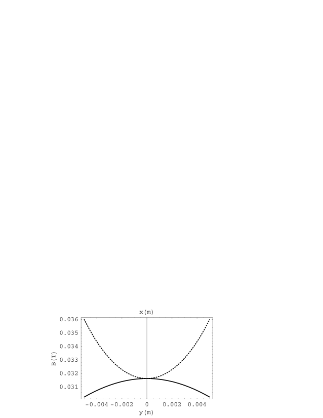
Figure 7: Transverse spatial distribution of magnetic field along the $x$-axis (dashed line) and the $y$-axis (solid line) at the output plave of the MD-Zeeman slower at $z=25.7\,$cm.

Figure 8: Spatial distribution of maximum gradient of magnetic field inside the slower, which provides continuous deceleration of atoms (dashed line). The computed distribution of the magnetic field gradient of the magnetic field of the considered MD-Zeeman slower (solid line).

The well known limit on the maximal slope steepness of the magnetic field of a Zeeman slower is given by the ratio

$$\frac{dB(z)}{dz}<\frac{\hbar ka_{max}(z)}{\mu_{B}v(z)}.$$ (12)

This formula is derived from the condition that the local deceleration rate $a(z)$ can’t exceed $a_{max}(z)$. This condition is true, but not complete. If the local deceleration rate $a(z)$ exceeds the maximum value $a_{max}(z)$, but only for a short period of time $\delta t$, the atoms can still be further decelerated along the stable velocity-trajectory of a Zeeman slower. The maximal duration of this time can be estimated from the ratio $(a(z)-a_{max}(z))\delta t=v_{res}(z)-v(z)$, which means that the exceeding acceleration should be able to accelerate an atom during the time $\delta t$ from its equilibrium velocity to the resonant velocity, at which atom is lost from the further deceleration process. The dashed line in fig. 8 shows the spatial distribution of the accepted maximal local gradient of the magnetic field, computed numerically from the eq. 12 for a decelerated atom. The solid line represents the actual gradient of the magnetic field, produced by an array of magnetic dipoles of the MD-Zeeman slower.

Figure 9: The optimal magnetic field distribution (solid line) and the simulated field distribution of the slower composed of finite-size neodymium magnets surrounded with an iron magnetic shield.

The magnetic moment of a real magnet is determined as $M=B_{i}V/\mu_{0}$, where $B_{i}$ is intrinsic induction and $V$ is the total volume of the magnet. The value $M=1.86\,$Am² in the examples considered above corresponds to a cylindrical neodymium magnet with $B_{i}=1.1\,$T, diameter $1.5\,$cm and height $1.2\,$cm. Figure 9 shows a precise calculation of the MD-Zeeman slower based on such finite-size magnets performed with the finite element analysis software COMSOL. In these calculations the distances of the centers of the magnets from the axis of the slower were taken exactly the same as in the MD model described above. The positions of the iron magnetic shields were also the same as in fig. 6.

IV Outlook

The mechanical construction of such a slower can be rather simple and inexpensive. It can be a box made of iron or some other material of high magnetic permeability, which serves as a frame for a two sets of screws with cylindrical magnets attached to their bottoms. The box is used both for holding the screws and for magnetic screening of the slower. In such a construction the distances of the individual magnets from the axis of the slower can be adjusted by rotation of the corresponding screws, without changing their axial positions.

In the considered MD-Zeeman slower all the magnets of the same size were used. In practice it make sense to use in the centre of the slower smaller magnets placed closer to the axis of the slower, which will make the whole construction more compact.

The maximum flux of cold atoms produced by a Zeeman slower is usually decreased by a transverse heating of the slowed atoms via the spontaneous scattering of the cooling light. This heating can be partially compensated by introducing additional sections, where the transverse motion of atoms is cooled down with additional transverse laser beams. This makes possible to increase the total flux of the cold atoms typically by one order of the magnitude or more. Such a transverse cooling of the atoms can be performed before Slowe , after Lison or in between the two sections Joffe of a standard Zeeman coil magnet. The problem is that the access to the atoms in the transverse direction is normally completely blocked by the coils. In a transverse MD-Zeeman slower the two arrays of compact magnets are placed from the two sides of the atomic beam and it is easy to get access to it on the whole length of the atomic beam. Therefore, for a MD-Zeeman slower it is possible to cool atoms transversely along the whole length of the slower.

Finally, a few words on the operation of the transverse MD-Zeeman slower. A transverse slower uses linearly polarized light, which can be presented as a linear superposition of two ($\sigma^{+}$ and $\sigma^{-}$) circularly polarized components. Therefore, only one-half of the total light intensity is in resonance with the right Zeeman transition of the decelerated atoms. An additional complication arises when a Zeeman splitting of magnetic sublevels of the ground state of an atom is comparable to the natural linewidth of the atomic transition. As it was recently shown in Balykin , a transverse Zeeman slower for Rb atoms demands quite some additional light power to make it work in the presence of the optical pumping between the split magnetic sublevels of the ground state. Fortunately, the Zeeman splitting of the ground state of the atoms from the earth-metal group is very small Lemonde2 . That is why such a transverse MD-Zeeman slower is very promising for use in an optical atomic clock based on such atoms.

V Conclusion

A standard theory of a Zeeman slower is extended to a case of a nonuniform intensity distribution of the cooling light. A way to include the absorption of the cooling light into the calculation of the optimal magnetic field of a Zeeman slower is described. It is shown that in that case the numerical simulation of the acceleration of atoms starting from their final position in the slower and calculating in the backwards direction is preferable. A new design parameter $\epsilon$ instead of the standard one $\eta$ parameter is proposed. The main advantage of such a definition is that the most optimal cooling of the decelerated atoms is reached at exactly $\epsilon=0.75$.

A transverse Zeeman slower composed of an array of discrete compact magnets is proposed and a simple model of such a slower is developed. As an example, a compact transverse Zeeman slower for Sr atoms has been calculated in presence of 50% absorption of the cooling light. The validity of the simple MD model of the slower for a slower composed of finite-size magnets has been confirmed with precise numerical calculations.

- (1) W. D. Phillips and H. Metcalf, Phys. Rev. Lett. 48, 596 (1982).
- (2) C. Slowe, L. Vernac and L. V. Hau, Rev. Sci. Instr. 76, 103101 (2005).
- (3) E. Riis, D. S. Weiss, K. A. Moler and S. Chu, Phys. Rev. Lett. 64, 1658 (1990).
- (4) K. Dieckmann, R. J. C. Spreeuw, M. Weidemüller and J. T. M. Walraven, Phys. Rev. A 58, 3891 (1998).
- (5) Yu.B. Ovchinnikov, Opt. Comm. 249, 473 (2005).
- (6) J. Schoser, A. Batär, R. Löw, V. Schweikhard, A. Grabowski, Yu.B. Ovchinnikov, and T. Pfau, Phys. Rev. A 66, 023410 (2002).
- (7) C. Adler, F. Narducci, C. Sukenik, J. Mulholland, S. Goodale, Bull. APS 51, 51 (2006).
- (8) R. J. Napolitano, S. C. Zilio and V. S. Bagnato, Opt. Comm. 80, 110 (1990).
- (9) P. A. Molenaar, P. Van der Straten, H. G. M. Heideman and H. Metcalf, Phys. Rev. A 55, 605 (1997).
- (10) M. E. Firmino, C. A. Faria Leite, S. C. Zilio and V. S. Bagnato, Phys. Rev. A 41, 4070 (1990).
- (11) I. Courtillot, A. Quessada, R. P. Kovacich, J-J. Zondy, A. Landragin, A. Clairon and P. Lemonde, Opt. Let. 28 468 (2003).
- (12) F. Lison, P. Schuh, D. Haubrich and D. Meschede, Phys. Rev. A 61, 013405 (1999).
- (13) M. A. Joffe, W. Ketterle, A. Martin and D. E. Pritchard, J. Opt. Soc. Am. B 10, 2257 (1993).
- (14) P. N. Melentiev, P. A. Borisov and V. I. Balykin, J. Exp. Theor. Phys. 98 667 (2004).
- (15) I. Courtillot, A. Quessada-Vial, A. Brusch, D. Kolker, G.D. Rovera and P. Lemonde, Eur. Phys. J. D 33, 161 (2005).