Explicit wave-averaged primitive equations using a Generalized Lagrangian Mean

Abstract

The generalized Langrangian mean theory provides exact equations for general wave-turbulence-mean flow interactions in three dimensions. For practical applications, these equations must be closed by specifying the wave forcing terms. Here an approximate closure is obtained under the hypotheses of small surface slope, weak horizontal gradients of the water depth and mean current, and weak curvature of the mean current profile. These assumptions yield analytical expressions for the mean momentum and pressure forcing terms that can be expressed in terms of the wave spectrum. A vertical change of coordinate is then applied to obtain $glm2z$-RANS equations (55) and (57) with non-divergent mass transport in cartesian coordinates. To lowest order, agreement is found with Eulerian-mean theories, and the present approximation provides an explicit extension of known wave-averaged equations to short-scale variations of the wave field, and vertically varying currents only limited to weak or localized profile curvatures. Further, the underlying exact equations provide a natural framework for extensions to finite wave amplitudes and any realistic situation. The accuracy of the approximations is discussed using comparisons with exact numerical solutions for linear waves over arbitrary bottom slopes, for which the equations are still exact when properly accounting for partial standing waves. For finite amplitude waves it is found that the approximate solutions are probably accurate for ocean mixed layer modelling and shoaling waves, provided that an adequate turbulent closure is designed. However, for surf zone applications the approximations are expected to give only qualitative results due to the large influence of wave nonlinearity on the vertical profiles of wave forcing terms.

, ,

1 Introduction

From wave-induced mixing and enhanced air-sea interactions in deep water, to wave-induced currents and sea level changes on beaches, the effects of waves on ocean currents and turbulence are well documented (e.g. Battjes 1988, Terray et al. 1996). The refraction of waves over horizontally varying currents is also well known, and the modifications of waves by vertical current shears have been the topic of a number of theoretical and laboratory investigations (e.g. Biesel 1950, Peregrine 1976, Kirby and Chen 1989, Swan et al. 2001), and field observations (e.g. Ivonin et al. 2004). In spite of this knowledge and the importance of the topic for engineering and scientific applications, ranging from navigation safety to search and rescue, beach erosion, and de-biasing of remote sensing measurements, there is no well established and generally practical numerical model for wave-current interactions in three dimensions.

Indeed the problem is made difficult by the difference in time scales between gravity waves and other motions. When motions on the scale of the wave period can be resolved, Boussinesq approximation of nearshore flows has provided remarkable numerical solutions of wave-current interaction processes (e.g. Chen et al. 2003, Terrile et al. 2006). However, such an approach still misses some of the important dynamical effects as it cannot represent real vertical current shears and their mixing effects (Putrevu and Svendsen 1999). This shortcoming has been partly corrected in quasi-three dimensional models (e.g. Haas et al. 2003), or multi-layer Boussinesq models (e.g. Lynnett and Liu 2005).

The alternative is of course to use fully three dimensional (3D) models, based on the primitive equations. These models are extensively used for investigating the global, regional or coastal ocean circulation (e.g. Bleck 2002, Shchepetkin and McWilliams 2003). An average over the wave phase or period is most useful due to practical constraints on the computational resources, allowing larger time steps and avoiding non-hydrostatic mean flows. Wave-averaging also allows an easier interpretation of the model result. A summary of wave-averaged models in 2 or 3 dimensions is provided in table 1.

Theory	averaging	momentum variable	main limitations
Phillips (1977)	Eulerian	total ($U$)	2D, $d\overline{u}/dz=0$
Garrett (1976)	Eulerian	mean flow ($U-M^{w}/D$)	2D, $d\overline{u}/dz=0$, $kh\gg 1$
Smith (2006)	Eulerian	mean flow ($U-M^{w}/D$)	2D, $d\overline{u}/dz=0$
GLM (A&M 1978a)	GLM	mean flow ($\overline{\mathbf{u}}^{L}-\mathbf{P}$)	none (exact theory)
aGLM (A&M 1978a)	GLM	total ($\overline{\mathbf{u}}^{L}$)	none (exact theory)
Leibovich (1980)	Eulerian	mean flow ($\overline{\mathbf{u}}^{L}-\mathbf{P}$)	2nd order, $\nu$ constant
Jenkins (1987)	GLM	mean flow ($\overline{\mathbf{u}}^{L}-\mathbf{P}$)	2nd order, horizontal uniformity
Groeneweg (1999)	GLM	total ($\overline{\mathbf{u}}^{L}$)	2nd order
Mellor (2003)	following $\xi_{3}$	total ($\overline{\mathbf{u}}^{L}$)	2nd order, flat bottom
MRL04	Eulerian	mean flow ($\overline{u}$)	below troughs, $\overline{u}\ll C$, $\nu=0$
NA07	Eulerian	mean flow ($\overline{u}$)	below troughs, 2nd order, $kH\ll 1$
present paper	GLM	mean flow ($\overline{\mathbf{u}}^{L}-\mathbf{P}$)	2nd order

Table 1: Essential attributes of some general wave-current coupling theories. See list of symbols for details (table 2 at the end of the paper). Although Mellor (2003) derived his wave-averaged equations with spatially varying wave amplitudes, his use of flat-bottom Airy wave kinematics is inconsistent with the presence of bottom slopes (see ARB07). MRL04 stands for McWilliams et al. (2004) and NA2007 stands for Newberger and Allen (2007).

1.1 Air-water separation

In 3D, problems arise due to the presence of both air and water in the region between wave crests and troughs. Various approaches to the phase or time averaging of flow properties are illustrated in figure 1 (see also Ardhuin et al. 2007b, hereinafter ARB2007). For small amplitude waves, one may simply take a Taylor expansion of mean flow properties (e.g. McWilliams et al. 2004, hereinafter MRL04). Using a decomposition of the non-linear advection term in the equations of motion $\mathbf{u}\mbox{\boldmath$\cdot$}\mbox{\boldmath$\nabla$}\mathbf{u}=\mbox{\boldmath$\nabla$}u^{2}+\mathbf{u}\times\mbox{\boldmath$\nabla$}\mathbf{u}$, McWilliams et al. (2004, see also Lane et al. 2007) obtained a relatively simple set of equation for conservative wave motion over sheared currents, for a given choice of small parameters. These parameters include the surface slope $\varepsilon_{1}=k_{0}a_{0}$ and the ratio of the wavelength and scale of evolution of the wave amplitucde. Further, these equations were derived with a scaling corresponding to a non-dimensional depth $k_{0}h_{0}$ of order 1, with $k_{0}$, $a_{0}$ and $h_{0}$ typical values of the wavenumber, wave amplitude and water depth, respectively. These authors also assumed that the current velocity was of the same order as the wave orbital velocity, both weaker than the phase speed by a factor $\varepsilon_{1}$. That latter assumption may generally be relaxed since the equations of motion are invariant by a change of reference frame, so that only the current vertical shear may need to be small compared to the wave radian frequency, provided that the current, water depth and wave amplitudes are slowly varying horizontally.

For waves of finite amplitude, a proper separation of air and water in the averaged equations of motion requires a change of coordinates that maps the moving free surface to a level that is fixed, or at least slowly varying. This is usual practice in air-sea interaction studies, and it has provided approximate solutions to problems such as wind-wave generation or wave-turbulence interactions (e.g. Jenkins 1986, Teixeira and Belcher 2002) but it brings some complications. The most simple change of coordinate was recently proposed by Mellor (2003), but it appears to be impractical in the presence of a bottom slope because its accurate implementation requires the wave kinematics to first order in the wave slope (Ardhuin et al., 2007b, hereinafter ARB07).

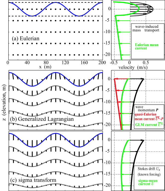
Figure 1: Averaging procedures (left) and examples of resulting velocity profiles (right) in the case of (a) Eulerian averages (e.g. Rivero and Sanchez-Arcilla 1995, McWilliams et al. 2004), (b) the Generalized Lagrangian Mean (Andrews and McIntyre 1978a), and (c) sigma transform (Mellor 2003, AJB07). The thick black bars connect the fixed points $\mathbf{x}$ where the average field is evaluated, to the displaced points $\mathbf{x}+\xi$ where the instantaneous field is evaluated. For averages in moving coordinates the points $\mathbf{x}+\xi$ at a given vertical level $\xi$ are along the gray lines. The drift velocity is the sum of the (quasi-Eulerian) current and the wave-induced mass transport. In the present illustration an Airy wave of amplitude 3 m and wavelength 100 m in 30 m depth, is superimposed on a hypothetical current of velocity $u(z)=-0.5-0.01z$ m/s for all $z<\zeta(\mathbf{x})$. The current profile is not represented in (c) since it is not directly given in Mellor’s theory, although it can obviously be obtained by taking the difference of the other two profiles.

1.2 Separation of wave and current momentum fluxes

Another approach is to use one of the two sets of exact averaged equations derived by Andrews and McIntyre (1978a). Groeneweg (1999) successfully used the second set, the alternative Generalized Lagragian Mean equations (aGLM), approximated to second order in wave slope, for the investigation of current profile modifications induced by waves (see also Groeneweg and Klopman 1998, Groeneweg and Battjes 2003). This work was also loosely adapted for engineering use in the numerical model Delft3D (Walstra et al. 2001).

However, aGLM equations describe the evolution of the total flow momentum, which includes the wave pseudo-momentum per unit mass $\mathbf{P}$. That vector quantity is generally close to the Lagrangian Stokes drift $\overline{\mathbf{u}}^{S}$ (see below), and it is not mixed by turbulence, unlike the mean flow momentum. Further, $\mathbf{P}$ is carried by the wave field at the group velocity, which is typically one order of magnitude faster than the drift velocity. Thus bundling $\mathbf{P}$ with the rest of the momentum may lead to large errors with the turbulence closure. Other practical problems arise due to the strong surface shear of $\mathbf{P}$ and $\overline{\mathbf{u}}^{S}$ (e.g. Rascle et al. 2006) whereas the quasi-Eulerian current is relatively uniform in deep water (e.g. Santala and Terray 1992). Thus solving for the total momentum (including $\mathbf{P}$) requires a high resoltion near the surface. Finally, a consistent expression of the aGLM equations with a sloping bottom and wave field gradients is difficult due to the divergence of vertical fluxes of momentum (vertical radiation stresses) that must be expressed to first order in all the small parameters that represent the slow wave field evolution (bottom slope, wave energy gradients, current shears…). This same problem arises with Mellor’s (2003) equations and is discussed in ARB07.

The first set of GLM equations describes the evolution of the quasi-Eulerian current only, and, just like the decomposition of $\mathbf{u}\mbox{\boldmath$\cdot$}\mbox{\boldmath$\nabla$}u$ used by MRL04, it does not require the evaluation of these vertical radiation stresses. These equations were used by Leibovich (1980) to derive the Craik-Leibovich equations that is the basis of theories for Langmuir circulations. However, in that work he did not attempt an explicit integration of the GLM set, and thus did not express the wave forcing terms from wave amplitudes or spectra. The general mathematical structure of the GLM equations and their conservatin properties are also well detailed in Holm (2002) and references therein.

Further, the GLM flow is generally divergent as the averaging operator introduces an implicit change of the vertical coordinate. This question has been largely overlooked by previous users of GLM theory (Leibovich 1980, Groeneweg 1999). Further, in order to be implemented in a numerical model, the wave-induced forcing terms must be made explicit using approximate solutions for wave-induced motions and pressure. We will assume that the slowly varying spectrum is known, typically provided by a wave model. Given the degree of accuracy attained by modelled wave spectra in a wide variety of conditions this is generally appropriate (e.g. Herbers et al. 2000, Ardhuin et al. 2003, 2007, Magne et al. 2007). We note in passing that no explicit and theoretically satisfying theory is available for the transport of the wave action spectrum over vertically and horizontally sheared currents. Indeed, the exact theory of Andrews and McIntyre (1978b) is implicit and would require an explicit approximation of the wave action from know wave kinematics, similar to the approximation of the wave pseudo-momentum performed here.

The goal of the present paper is to provide a practical and accurate method for wave-current coupling that is general enough for applications ranging from the ocean mixed layer to, possibly, the surf zone. GLM equations, for the reasons listed above, are a good candidate for this application. Although not as simple as an Eulerian average, the GLM operator is capable of properly separating air and water in the crest to trough region, leading to physically understandable definitions of mean properties on either side of the air-sea interface. The practical use of GLM requires some approximations and transformations. We provide in section 2 a derivation of explicit and approximate $glm2z$-RANS equations. Given the large literature on the subject, we explore in section 3 the relationships between GLM, aGLM and other forms of wave-averaged 3D and depth-integrated 2D equations. A preliminary analysis of the expected errors due to the approximations are provided in section 4, and conclusions follow in section 5. Full numerical solutions using the $glm2z$-RANS equations will be reported elsewhere, in particular in the doctorate thesis of Nicolas Rascle.

2 glm2-RANS equations

2.1 Generalities on GLM and linear wave kinematics

We first define the Eulerian average $\overline{\phi\left({\mathbf{x}},t\right)}$ of $\phi\left({\mathbf{x}},t\right)$, where the average may be an average over phase, realizations, time $t$ or space. We now take this average at displaced positions $\mathbf{x}+\xi$, with $\xi=(\xi_{1},\xi_{2},\xi_{3})$ a displacement vector, and we defining the velocity ${\mathbf{v}}$ at which the mean position is displaced when the actual position moves at the fluid velocity $\mathbf{u}(\mathbf{x}+\xi)$. One obtains the corresponding GLM of $\phi$

$$\overline{\phi(\mathbf{x},t)}^{L}=\overline{\phi(\mathbf{x}+\xi,t)}$$ (1)

by choosing the displacement field $\xi$ so that

• the mapping $\mathbf{x}\rightarrow\mathbf{x}+\xi$ is invertible

• $\overline{\xi\left({\mathbf{x}},t\right)}=0$

• $\overline{{\mathbf{v}}\left({\mathbf{x}},t\right)}={\mathbf{v}}\left({\mathbf{x}},t\right)$, which gives ${\mathbf{v}}=\overline{\mathbf{u}(\mathbf{x},t)}^{L}$.

Such a mapping is illustrated in figure 1.c for linear waves. Lagrangian perturbations are logically defined as the field minus its average, i.e.,

$$\overline{\phi(\mathbf{x},t)}^{l}=\phi(\mathbf{x}+\xi,t)-\overline{\phi(\mathbf{x},t)}^{L}=\phi(\mathbf{x}+\xi,t)-\overline{\phi(\mathbf{x}+\xi,t)}.$$ (2)

Here we shall take our Eulerian average to be a phase average. Given any Eulerian flow field $\mathbf{u}(\mathbf{x},t)$, one may define a first displacement by

$$\xi^{\prime}(\mathbf{x},t,\Delta t)=\int_{t}^{t+\Delta t}\mathbf{u}(\mathbf{x}+\xi^{\prime}(\mathbf{x},t,t^{\prime}-t),t^{\prime})\mathrm{d}t^{\prime}.$$ (3)

The mean drift velocity is defined as ${\mathbf{v}}(\mathbf{x},t)=\lim_{\Delta t\rightarrow 0}\overline{\xi^{\prime}(\mathbf{x},t,\Delta t)}/(\Delta t)$. The GLM displacement field is then given by $\xi=\xi^{\prime}-{\mathbf{v}}t-\overline{\xi^{\prime}-{\mathbf{v}}t}$. This construction of ${\mathbf{v}}$ and $\xi$ guarantees that the required properties are obtained, provided that the limit $\Delta t\rightarrow 0$ commutes with the averaging operator. For periodic motions one may also take ${\mathbf{v}}=\overline{\left(\xi^{\prime}(t+T^{L})-\xi^{\prime}(t)\right)}/(T^{L})$, with $T^{L}$ the Lagrangian wave period (the time taken by a water particle to return to the same wave phase). This definition will be used for Miche waves in section 4.2.

Clearly GLM differs from the Eulerian mean. The difference between the two is given by the Stokes correction (Andrews et McIntyre 1978a). Below the wave troughs, the Stokes correction for the velocity is the Stokes drift, by definition,

$$\overline{\mathbf{u}}^{S}\equiv\overline{{\mathbf{u}}}^{L}-\overline{\mathbf{u}}.$$ (4)

More generally, for a continuously differentiable field $\phi$ the Stokes correction is given by (Andrews and McIntyre 1978a, equation 2.27),

$$\overline{\phi}^{L}\equiv\overline{\phi}+\overline{\phi}^{S}=\overline{\phi}+\overline{\xi_{j}\frac{\partial\phi}{\partial x_{j}}}+\frac{1}{2}\overline{\xi_{j}\xi_{k}}\frac{\partial^{2}\overline{\phi}}{\partial x_{j}\partial x_{k}}+O\left(\max_{i,j,k}\left\{\frac{\partial^{3}\overline{\phi}}{\partial x_{i}\partial x_{j}\partial x_{k}}\right\}|\xi|^{3}\right),$$ (5)

with an implicit summation over repeated indices.

The GLM average commutes with the Lagrangian derivative, thus the GLM velocity $\overline{{\mathbf{u}}}^{L}$ is the average drift velocity of water particles. One should however be careful that the GLM average does not commute with most differential operators, for example the curl operator. Indeed the GLM velocity of irrotational waves is rotational, which is clearly apparent in the vertical shear of the Stokes drift (see also Ardhuin and Jenkins 2006 for a calculation of the lowest order mean shears $\overline{\partial u_{\alpha}/\partial z}^{L}$ and $\overline{\partial u_{3}/\partial x}^{L}$).

One of the interesting aspects of GLM theory is that it clearly separates the wave pseudo-momentum $\mathbf{P}$ from the quasi-Eulerian mean momentum $\widehat{{\mathbf{u}}}=\overline{{\mathbf{u}}}^{L}-\mathbf{P}$. This is a key aspect for numerical modelling since $\mathbf{P}$ is transported by the wave field at the group velocity, of the order of 5 m s^-1 in deep water, while $\widehat{{\mathbf{u}}}$ is transported at the much slower velocity $\overline{{\mathbf{u}}}^{L}$. $\mathbf{P}$ is defined by (Andrews and McIntyre 1978a, eq. 3.1),

$$P_{i}=-\overline{\xi_{j,i}\left(u^{l}_{j}+\epsilon_{jkl}f_{k}\xi_{l}/2\right)},$$ (6)

where $\epsilon_{ijk}A_{j}B_{k}$ is the $i$-component of the vector product $\mathbf{A}\times\mathbf{B}$, and $f_{k}/2$ is the $k$-component of the rotation vector of the reference frame. In the applications considered here the effect of rotation can be neglected in (6) due to the much larger rotation period of the Earth compared to the wave period. We will thus take

$$P_{i}=-\overline{\xi_{j,i}u^{l}_{j}}.$$ (7)

For practical use, the GLM equations have to be closed by specifying the wave-induced forcing terms. In order to give explicit approximations for the wave-induced effects, we will approximate the wave motion as a sum of linear wave modes, each with a local wave phase $\psi$ giving the local wave number $\mathbf{k}=(k_{1},k_{2})=\mbox{\boldmath$\nabla$}\psi$, and radian frequency $\omega=-\partial\psi/\partial t$, and an intrinsic linear wave radian frequency $\sigma=\left[gk\tanh(kD)\right]^{1/2}=\omega-\mathbf{k}\mbox{\boldmath$\cdot$}\mbox{\boldmath$U$}_{A}$, where $\mbox{\boldmath$U$}_{A}$ is the phase advection velocity, $D$ is the local mean water depth, and $g$ the acceleration due to gravity and Earth rotation. Defining $h(x_{1},x_{2})$ as the local depth of the bottom and $\zeta(x_{1},x_{2},t)$ as the free surface elevation, one has $D=\overline{\zeta}+h$. We assume that the wave slope $\varepsilon_{1}=\max\left(|\mbox{\boldmath$\nabla$}\zeta|\right)$ is small compared to unity (this will be our first hypothesis H1), with $\nabla$ denoting the horizontal gradient operator. We also restrict our investigations to cases for which the Ursell number is small $Ur=(a/D)/(kD)^{2}<1$ (this is hypothesis H2). We further restrict our derivations to first order in the slow spatial scale $\varepsilon_{2}$. That small parameter may be defined as the maximum of the slow spatial scales $|(\partial a/\partial x)/(ka)|$, $|(\partial\overline{u}/\partial x)/(\sigma)|$, $|(\partial D/\partial x)|$, and time scales $|(\partial a/\partial t)/(\sigma a)|$, $|k(\partial\widehat{u}/\partial t)/(\sigma)^{2}$, and $|(\partial D/\partial t)k/\sigma|$ (hypothesis H3). It will also appear that the current profile may cause some difficulties. Since we have already assumed a small wave steepness we may use Kirby and Chen’s (1989) results, giving the dispersion relation

$$\omega=\sigma+k_{\alpha}\int_{-h}^{\overline{\zeta}}\widehat{u}_{\alpha}\frac{2k\cosh\left[2k(z+h)\right]}{\sinh(2kD)}\mathrm{d}z+O(\varepsilon_{3}),$$ (8)

where $\alpha$ is a dummy index representing any horizontal component 1 or 2, and the summation is implicit over repeated indices. The index 3 will represent the vertical components positive upwards, along the direction $z=x_{3}$. In particular we shall assume that their correction to the lowest order stream function (their eq. 23) is relatively small, which may be obtained by requiring that the curvature of the current is weak or concentrated in a thin boundary layer, i.e. $\varepsilon_{3}\ll 1$ (hypothesis H4) with

$$\varepsilon_{3}=\frac{1}{\omega\sinh(kD)}\int_{-h}^{\zeta}\left|\frac{\partial^{2}\overline{u}}{\partial z^{2}}\right|\sinh\left[2k(z+h)\right]\mathrm{d}z.$$ (9)

For simplicity we will further require that $a^{2}\left[{\partial^{3}\overline{u}_{\alpha}}/{\partial z^{3}}/({\sigma})\right]\leq\varepsilon_{3}$ (hypothesis H5), which may be more restrictive than H4. Finally, we will neglect the vertical velocity $\widehat{w}$ in the vertical momentum equation for the mean flow momentum (i.e. we assume the mean flow to be hydrostatic, this is our hypothesis H6).

In the following we take $\varepsilon=\max{\varepsilon_{i},1\leqslant i\leqslant 3}$. The wave-induced pressure and velocity are given by

$$\widetilde{p} = \rho_{w}ga\left[F_{CC}\cos\psi+O(\varepsilon)\right]$$ (10)

$$\widetilde{u}_{\alpha} = a\sigma\frac{k_{\alpha}}{k}\left[F_{CS}\cos\psi+O(\varepsilon)\right]$$ (11)

$$\widetilde{u}_{3} = a\sigma\left[F_{SS}\sin\psi+O(\varepsilon)\right],$$ (12)

where $a$ is the local wave amplitude, $\rho_{w}$ is the water density, taken constant in the present paper. We have used the short-hand notations $F_{CC}=\cosh(kz+kD)/\cosh(kD)$, $F_{CS}=\cosh(kz+kD)/\sinh(kD)$, and $F_{SS}=\sinh(kz+kD)/\sinh(kD)$.

From now on, only the lowest order approximations will be given unless explicitly stated otherwise. In order to estimate quantities at displaced positions, the zero-mean displacement field is given by

$$u^{l}_{i} \equiv \mathbf{u}(\mathbf{x}+\xi)-\overline{u}^{L}_{i}$$ (13)

$$\simeq \widetilde{u}_{i}+\xi_{j}\frac{\partial\overline{u}_{i}}{\partial x_{j}}+\left(\xi_{j}\frac{\partial\widetilde{u}_{i}}{\partial x_{j}}-\overline{\xi_{j}\frac{\partial\widetilde{u}_{i}}{\partial x_{j}}}\right)+\frac{1}{2}\left(\xi_{j}^{2}-\overline{\xi_{j}^{2}}\right)\frac{\partial^{2}\overline{u}_{i}}{\partial x_{j}^{2}}.$$

Thanks to the definition of $\overline{u}^{L}$, we also have

$$u^{l}_{i}=\frac{\partial\xi_{i}}{\partial t}+\overline{u}^{L}_{j}\frac{\partial\xi_{i}}{\partial x_{j}}\simeq\frac{\partial\xi_{i}}{\partial t}+\overline{u}^{L}_{\alpha}\frac{\partial\xi_{i}}{\partial x_{\alpha}},$$ (14)

in which the vertical velocity has been neglected. The greek indices $\alpha$ and $\beta$ stand for horizontal components only.

To lowest order in the wave amplitude, the displacements $\xi_{i}$ and Lagrangian velocity perturbations $u^{l}_{i}$ are obtained from (13) and (14),

$$u_{3}^{l} = \widetilde{u}_{3}$$ (15)

$${\xi_{3}} = am\left[F_{SS}\cos\psi\right]$$ (16)

$$u_{\alpha}^{l} = \widetilde{u}_{\alpha}+{\xi_{3}}\frac{\partial\overline{u}_{\alpha}}{\partial z}+{\xi_{\beta}}\frac{\partial\overline{u}_{\alpha}}{\partial x_{\beta}}+O\left(\sigma ka^{2}\right)\cos 2\psi+O\left(a^{3}\frac{\partial^{2}\overline{u}_{\alpha}}{\partial z^{3}}\right)$$ (17)

$$\simeq a\left[\sigma\frac{k_{\alpha}}{k}F_{CS}+mF_{SS}\frac{\partial\overline{u}_{\alpha}}{\partial z}\right]\cos\psi$$ (18)

$${\xi_{\alpha}} = -am\left[\frac{k_{\alpha}}{k}F_{CS}+\frac{m}{\sigma}\frac{\partial\overline{u}_{\alpha}}{\partial z}F_{SS}\right]\sin\psi+O\left(\frac{a^{2}}{\sigma}\frac{\partial^{2}\overline{u}_{\alpha}}{\partial z^{2}}\right)\sin 2\psi$$ (19)

$$+O\left(\frac{a}{\sigma}\frac{\partial\overline{u}_{\alpha}}{\partial x_{\beta}}\right)\cos\psi+O\left(\frac{a^{3}}{\sigma}\frac{\partial^{2}\overline{u}_{\alpha}}{\partial z^{3}}\right),$$

The shear correction parameter $m$, arising from the time-integration of (14), is given by

$$m(\mathbf{x},\mathbf{k},z,t)=\frac{\sigma}{\omega-\mathbf{k}\mbox{\boldmath$\cdot$}\overline{\mathbf{u}}^{L}(\mathbf{x},z,t)}.$$ (20)

Based on (8) $m$ differs from 1 by a quantity of order $\sigma^{-1}\partial\overline{u}/\partial z$.

Using our assumption (H5) the last term in eq. (19) may be neglected. The last two term in eq. (17) have been neglected because they will give negligible $O(\varepsilon^{3})$ terms in $\mathbf{P}$, $\overline{\zeta}^{L}$ or other wave-related quantities, when multiplied by other zero-mean wave quantities.

Using the approximate wave-induced motions, one may estimate the Stokes drift

$$\overline{\mathbf{u}}^{S} \equiv \overline{{\mathbf{u}}}^{L}-\overline{u}\simeq\overline{\xi\mbox{\boldmath$\cdot$}\mbox{\boldmath$\nabla$}\widetilde{u}}+\frac{1}{2}\overline{\xi_{3}^{2}}\frac{\partial^{2}\overline{u}_{\alpha}}{\partial z^{2}}$$ (21)

$$= \frac{ma^{2}}{4\sinh^{2}(kD)}\left[2\sigma{\mathbf{k}}\cosh(2kz+2kh)+{\mathbf{k}}m\sinh(2kz+2kh)\frac{\mathbf{k}}{k}\mbox{\boldmath$\cdot$}\frac{\partial\overline{\mathbf{u}}}{\partial z}\right.$$

$$+\left.\frac{\partial^{2}\overline{\mathbf{u}}}{\partial z^{2}}\sinh^{2}(kz+kh)\right],$$

the horizontal wave pseudo-momentum

$$P_{\alpha} = -\overline{\frac{\partial\xi_{\beta}}{\partial x_{\alpha}}u_{\beta}^{l}}-\overline{\frac{\partial\xi_{3}}{\partial x_{\alpha}}w^{l}}$$ (22)

$$\simeq \frac{ma^{2}}{4\sinh^{2}(kD)}\left[2\sigma k_{\alpha}\cosh(2kz+2kh)+2k_{\alpha}m\sinh(2kz+2kh)\frac{k_{\alpha}}{k}\mbox{\boldmath$\cdot$}\frac{\partial\overline{\mathbf{u}}}{\partial z}\right.$$

$$+2m^{2}\frac{k_{\alpha}}{\sigma}\sinh^{2}(kz+kh)\left.\left(\frac{\partial\overline{\mathbf{u}}}{\partial z}\right)^{2}\right],$$

and the GLM position of the free surface

$$\overline{\zeta}^{L}=\overline{\zeta}+\overline{\zeta}^{S}=\overline{\zeta}+\frac{\partial\zeta}{\partial x_{\alpha}}\xi_{\alpha}|_{z=\overline{\zeta}}=\overline{\zeta}+\frac{ma^{2}}{2}\left[\frac{k}{\tanh kD}+\frac{m\mathbf{k}}{\sigma}\mbox{\boldmath$\cdot$}\frac{\partial\overline{\mathbf{u}}}{\partial z}|_{z=\overline{\zeta}}\right].$$ (23)

Thus the GLM of vertical positions in the water is generally larger than the Eulerian mean of the position of the same particles (see also McIntyre 1988). This is easily understood, given that there are more particles under the crests than under the troughs (figure 1.c). As a result, the original GLM equations are divergent ($\mbox{\boldmath$\nabla$}\mbox{\boldmath$\cdot$}\overline{u}^{L}\neq 0$) and require a coordinate transformation to yield a non-divergent velocity field. That transformation is small, leading to a relative correction of order $\varepsilon_{1}^{2}$. That transformed set of equation is a modified primitive equation that may be implemented in existing ocean circulation models.

The horizontal component of the wave pseudo-momentum $P_{\alpha}$ differs from the Stokes drift $\overline{u}_{\alpha}^{S}$ due to the current vertical shear. Therefore the quasi-Eulerian mean velocity $\widehat{u}_{\alpha}=\overline{u}^{L}_{\alpha}-P_{\alpha}$ also differs from the Eulerian mean velocity $\overline{u}_{\alpha}=\overline{u}^{L}_{\alpha}-\overline{u}_{\alpha}^{S}$

$$\widehat{u}_{\alpha}=\overline{u}_{\alpha}+\frac{1}{2}\overline{\xi_{3}^{2}}\frac{\partial^{2}\overline{u}_{\alpha}}{\partial z^{2}}+O(\varepsilon_{3}).$$ (24)

The vertical wave pseudo-momentum $P_{3}=0$ is, at most, of order $\sigma\varepsilon^{3}/k$. Although it may be neglected in the momentum equation, it plays an important role in the mass conservation equation, and will thus be estimated from $P_{\alpha}$. In particular, for $m=1$ and in the limit of small surface slopes, it is straightforward using (7) to prove that $\mathbf{P}$ is non-divergent and such that $\mathbf{P}\mbox{\boldmath$\cdot$}\mathbf{n}=0$ at $z=-h$, with $\mathbf{n}$ the normal to the bottom. This gives,

$$P_{3}=-P_{\alpha}(-h)\frac{\partial h}{\partial x_{\alpha}}-\int_{-h}^{z}\frac{\partial P_{\alpha}(z^{\prime})}{\partial x_{\alpha}}\mathrm{d}z^{\prime}.$$ (25)

Although this equality is not obvious for $m\neq 1$ and nonlinear waves, corrections to (25) are expected to be only of higher order ,in particular once $\mathbf{P}$ is transformed to $z$ coordinates. Indeed, in the absence of a mean flow $\mathbf{P}=\overline{\mathbf{u}}^{L}$ and it is non-divergent (see section 2.1.1).

2.1.1 glm2-RANS equations

The velocity field is assumed to have a unique decomposition in mean, wave and turbulent components $\mathbf{u}=\overline{\mathbf{u}}+\widetilde{\mathbf{u}}+\mathbf{u}^{\prime}$, with $\left<{\mathbf{u}^{\prime}}\right>=0$, the average over the flow realizations for prescribed wave phases. The turbulence will be assumed weak enough so that its effect on the sea surface position is negligible. We note ${\mathbf{X}}$ the divergence of the Reynolds stresses, i.e. $X_{i}=\partial\left<u^{\prime}_{i}u^{\prime}_{j}\right>/\partial x_{j}$, and we apply the GLM average to the Reynolds-Average Navier-Stokes equations (RANS). We shall now seek an approximation to the GLM momentum equations by retaining all terms of order $\rho_{w}g\varepsilon^{3}$ and larger in the horizontal momentum equation, and all terms of order $\rho_{w}g\varepsilon^{2}$ in the vertical momentum equation. The resulting equations, that may be called the ”glm2-RANS” equations, are thus more limited in terms of wave nonlinearity than the Eulerian mean equations of MRL04. At the same time, random waves are considered here and that the mean current may be larger than the wave orbital velocity. Indeed we make no hypothesis on the current magnitude, but only on the horizontal current gradients and on the curvature of the current profile. The present derivation differs from that of Groeneweg (1999) by the fact that we use the GLM instead of the aGLM equations (see table 1). The name for these equations is loosely borrowed from Holm (2002) who instead derived an approximate Lagrangian to obtain the momentum equation, and did not include turbulence.

In order to simplify our calculations we shall use the form of the GLM equations given by Dingemans (1997, eq. 2.596) with $\rho_{w}$ constant, which, among other things, removes terms related to the fluid thermodynamics. The evolution equation for the quasi-Eulerian velocity $\widehat{\mathbf{u}}$ is,

$$\overline{D}^{L}\widehat{u}_{i}+\epsilon_{i3j}f_{3}\overline{u}^{L}_{j}+\frac{\partial}{\partial x_{i}}\left(\frac{\overline{p}^{L}}{\rho_{w}}-\frac{\overline{u^{l}_{j}u^{l}_{j}}}{2}\right)-\widehat{X}_{i}+g\delta_{i3}=P_{j}\frac{\partial\overline{u}^{L}_{j}}{\partial x_{i}},$$ (26)

where the Lagrangian derivative $D^{L}$ is a derivative following the fluid at the Lagrangian mean velocity $\overline{u}^{L}$, $p$ is the full dynamic pressure, $\delta$ is Kronecker’s symbol, and the viscous and/or turbulent force $\widehat{\mathbf{X}}$ is defined by

$$\widehat{X}_{i}=\overline{X}^{L}_{i}+\overline{\frac{\partial\xi_{j}}{\partial x_{i}}\left(\overline{X}_{j}^{L}-X_{j}\right)}.$$ (27)

These exact equations will now be approximated using (10)-(16). We first evaluate the wave forcing terms in (26) using monochromatic waves, with a surface elevation variance $E=a^{2}/2$. The result for random waves follows by summation over the spectrum and replacing $E$ with the spectral density $E(\mathbf{k})$.

We first consider the vertical momentum balance, giving the pressure field. It should be noted that the Lagrangian mean Bernoulli head term $u^{l}_{j}u^{l}_{j}/2$ differs from its Eulerian counterpart $u^{\prime}_{j}u^{\prime}_{j}/2$ by a term $K_{2}$, which arises from the correlation of the mean current perturbation at the displaced position $\mathbf{x}+\xi$, with the wave-induced velocity, i.e. the second term in (17). Eqs. (10)–(16) give

$$\frac{1}{2}\left(u^{l}_{j}u^{l}_{j}\right)=\frac{gkE}{2}\left[F_{CC}F_{CS}+F_{SC}F_{SS}\right]+K_{2},$$ (28)

with

$$K_{2}=\widetilde{u}_{\alpha}\xi_{3}\frac{\partial\overline{u}_{\alpha}}{\partial z}+\frac{\xi_{3}^{2}}{2}\left|\frac{\partial\overline{\mathbf{u}}}{\partial z}\right|^{2}=E\frac{\sigma}{k}\mathbf{k}\mbox{\boldmath$\cdot$}\frac{\partial\widehat{\mathbf{u}}}{\partial z}mF_{CS}F_{SS}+\frac{E}{2}\left|\frac{\partial\overline{\mathbf{u}}}{\partial z}\right|^{2}m^{2}F^{2}_{SS}.$$ (29)

The vertical momentum equation (26) for $\widehat{w}=\widehat{u}_{3}$ is,

$$\frac{\partial\widehat{w}}{\partial t} + \widehat{w}\frac{\partial\widehat{w}}{\partial z}+P_{3}\frac{\partial\widehat{w}}{\partial z}+\left(\widehat{u}_{\beta}+P_{\beta}\right)\frac{\partial\widehat{w}}{\partial x_{\beta}}+\frac{1}{\rho_{w}}\frac{\partial\overline{p}^{L}}{\partial z}+g$$ (30)

$$= \frac{\partial}{\partial z}\left[\left(\overline{{\widetilde{u}}_{\alpha}{\widetilde{u}}_{\alpha}}+\overline{\widetilde{w}^{2}}\right)/2+K_{2}\right]+P_{\beta}\frac{\partial}{\partial z}\left(\widehat{u}_{\beta}+P_{\beta}\right)+P_{3}\frac{\partial}{\partial z}\left(\widehat{u}_{3}+P_{3}\right),$$

For small bottom slopes we may neglect the last term, but we rewrite it in order to compare with other sets of equations. Now using the lowest order wave solution (11)–(16), eq. (30) transforms to

$$\frac{1}{\rho_{w}}\frac{\partial}{\partial z}\left[\overline{p}^{L}+\rho_{w}gz-\rho_{w}\frac{\sigma^{2}E}{2}\left(F_{CS}^{2}+F_{SS}^{2}\right)-\rho_{w}K_{2}\right] = -\frac{\partial\widehat{w}}{\partial t}-\widehat{w}\frac{\partial\widehat{w}}{\partial z}$$

$$-\left(\widehat{u}_{\beta}+P_{\beta}\right)\frac{\partial\widehat{w}}{\partial x_{\beta}}+P_{\beta}\frac{\partial}{\partial z}\left(\widehat{u}_{\beta}+P_{\beta}\right) + P_{3}\frac{\partial}{\partial z}\left(\widehat{w}+P_{3}\right).$$ (31)

We add to both sides the depth-uniform term $-\sigma^{2}E\left(F_{CC}^{2}-F_{SS}^{2}\right)/2$, and integrate over $z$ to obtain

$$\frac{\overline{p(z)}^{L}}{\rho_{w}}=-g\left[\left(z-z_{s}\right)-kEF_{CC}F_{CS}\right]+K_{2}+K_{1}-\frac{gkE}{4\sinh(2kD)}$$ (32)

where the hydrostatic hypothesis (H6, see above) has be made for the mean flow. The depth-integrated vertical component of the vortex-like force $K_{1}$ is defined by

$$K_{1}=-\int_{z}^{\overline{\zeta}^{L}}P_{\beta}\frac{\partial}{\partial z^{\prime}}\left(\widehat{u}_{\beta}+P_{\beta}\right)\mathrm{d}z^{\prime}+\int_{z}^{\overline{\zeta}^{L}}P_{3}\frac{\partial}{\partial x_{\beta}}\left(P_{\beta}\right)\mathrm{d}z^{\prime},$$ (33)

where eq. (25) has been used. The integration constant $z_{s}$ is given by the surface boundary condition

$$\overline{p(\zeta)}^{L}=-\rho_{w}g\left(\overline{\zeta}^{L}-z_{s}-kEF_{CC}F_{CS}-K_{2}(\overline{\zeta}^{L})/g\right)=\overline{p}_{a}.$$ (34)

Using (23) we find that $z_{s}=\overline{\zeta}+\overline{p}_{a}/(\rho_{w}g)-K_{2}(\overline{(\zeta)}^{L})/g$ and (32) becomes

$$\frac{\overline{p}^{L}}{\rho_{w}}=\frac{\overline{p}^{H}}{\rho_{w}}+gkEF_{CC}F_{CS}+K_{1}+K_{2}-K_{2}(\overline{\zeta}^{L}),$$ (35)

with $p^{H}$ the hydrostatic pressure defined equal to the mean atmospheric pressure at the mean sea surface, $p^{H}=\rho_{w}g(\overline{\zeta}-z)+\overline{p}_{a}$.

Below the wave troughs the Stokes correction for the pressure (5) gives the Eulerian-mean pressure

$$\overline{p}=\overline{p}^{L}-\rho_{w}gkmE\left(F_{CS}F_{CC}+F_{SS}F_{SC}+\frac{\mathbf{k}}{k\sigma}\mbox{\boldmath$\cdot$}\frac{\partial\overline{\mathbf{u}}}{\partial z}mF_{SS}F_{CC}\right).$$ (36)

Thus equation (32) gives the following relationship, valid to order $\varepsilon_{1}^{2}$ below the wave troughs, between the Eulerian-mean pressure $\overline{p}$ and $\overline{p}^{L}$,

$$\overline{p} = p^{H}-\rho_{w}gkEF_{SS}F_{SC}+\rho_{w}\left(K_{1}-K_{2}(\overline{\zeta}^{L})+\frac{E}{2}\left|\frac{\partial\overline{\mathbf{u}}}{\partial z}\right|^{2}m^{2}F^{2}_{SS}\right)$$ (37)

$$+\rho_{w}gk(1-m)EF_{CC}F_{CS}.$$

For a spectrum of random waves, the modified pressure term that enters the horizontal momentum equation may be written as

$$\widehat{p}\equiv\overline{p}^{L}-\frac{\rho_{w}\overline{u^{l}_{j}u^{l}_{j}}}{2}-P_{j}\frac{\partial\overline{u}^{L}_{i}}{\partial z}=p^{H}+\rho_{w}S^{\mathrm{J}}+\rho_{w}S^{\mathrm{shear}},$$ (38)

with the depth-uniform wave-induced kinematic pressure term

$$S^{\mathrm{J}}=g\int_{\mathbf{k}}\frac{kE({\mathbf{k}})}{\sinh 2kD}{\mathrm{d}}{\mathbf{k}}$$ (39)

and a shear-induced pressure term, due to the integral of the vertical component of the vortex force $K_{1}$, and $K_{2}(\overline{\zeta}^{L})$,

$$S^{\mathrm{shear}} = -\int_{\mathbf{k}}E({\mathbf{k}})\left(\frac{\sigma}{k}k_{\beta}m\frac{\partial\widehat{u}_{\beta}(\overline{\zeta}^{L})}{\partial z}\tanh(kD)+\frac{m^{2}}{2}\left|\frac{\partial\widehat{\mathbf{u}}}{\partial z}(\overline{\zeta}^{L})\right|^{2}\right)\mathrm{d}\mathbf{k}$$ (40)

$$+ \int_{\mathbf{k}}\int_{z}^{\overline{\zeta}^{L}}\left[P_{3}(\mathbf{k})\frac{\partial P_{\beta}(z^{\prime},\mathbf{k})}{\partial x_{\beta}}-P_{\beta}(\mathbf{k})\frac{\partial\left[\widehat{u}_{\beta}(z^{\prime})+P_{\beta}(\mathbf{k})\right]}{\partial z^{\prime}}\right]\mathrm{d}z^{\prime}\mathrm{d}\mathbf{k}.$$

Now considering the horizontal momentum equations, we rewrite (26) for the horizontal velocity,

$$\frac{\partial\widehat{u}_{\alpha}}{\partial t} + \left(\widehat{u}_{\beta}+P_{\beta}\right)\frac{\partial\widehat{u}_{\alpha}}{\partial x_{\beta}}+\widehat{w}\frac{\partial\widehat{u}_{\alpha}}{\partial z}+\epsilon_{\alpha 3\beta}f_{3}\left(\widehat{u}_{\beta}+P_{\beta}\right)+\frac{1}{\rho_{w}}\frac{\partial p^{H}}{\partial x_{\alpha}}$$ (41)

$$= -\frac{\partial}{\partial x_{\alpha}}\left(S^{\mathrm{J}}+S^{\mathrm{shear}}\right)+P_{\beta}\frac{\partial\widehat{u}_{\beta}}{\partial x_{\alpha}}-P_{3}\frac{\partial\widehat{u}_{\alpha}}{\partial z}+\widehat{X}_{\alpha},$$

Grouping all $P_{\beta}$ terms, as in Garrett (1976 eq. 3.10 and 3.11), leads to an expression with the ‘vortex force’ $\epsilon_{\alpha 3\beta}\omega_{3}P_{\beta}$. This force is the vector product of the wave pseudo-momentum $\mathbf{P}$ and mean flow vertical vorticity $\omega_{3}$. Equation (41) transforms to

$$\frac{\partial\widehat{u}_{\alpha}}{\partial t}+\widehat{u}_{\beta}\frac{\partial\widehat{u}_{\alpha}}{\partial x_{\beta}}+\widehat{w}\frac{\partial\widehat{u}_{\alpha}}{\partial z} + \epsilon_{\alpha 3\beta}\left[f_{3}\widehat{u}_{\beta}+\left(f_{3}+\omega_{3}\right)P_{\beta}\right]+\frac{1}{\rho_{w}}\frac{\partial p^{H}}{\partial x_{\alpha}}$$ (42)

$$= -\frac{\partial}{\partial x_{\alpha}}\left(S^{\mathrm{J}}+S^{\mathrm{shear}}\right)-P_{3}\frac{\partial\widehat{u}_{\alpha}}{\partial z}+\widehat{X}_{\alpha}.$$

The vortex force is a momentum flux divergence that compensates for the change in wave momentum flux due to wave refraction over varying currents, and includes the flux of momentum resulting from $\widehat{\mathbf{u}}$ momentum advected by the wave motion (Garrett 1976).

The turbulent closure is the topic of ongoing research and will not be explicitly detailed here. We only note that it differs in principle from the closure of the aGLM equations of Groeneweg (1999), which could be extended to include the second term in eq. (27). A proper closure involves a full discussion of the distortion of turbulence by the waves when the turbulent mixing time scale is larger than the wave period (e.g. Walmsley and Taylor 1996, Janssen 2004, Teixeira and Belcher 2002). One should consider with caution the rather bold but practical assumptions of Groeneweg (1999) who used a standard turbulence closure to define the viscosity that acts upon the wave-induced velocities, or the assumption of Huang and Mei (2003) who assumed that the eddy viscosity instantaneously adjusts to the passage of waves. These effects may have consequences on the magnitude of wave attenuation through its interaction with turbulence, and the resulting vertical profile of $\widehat{X}_{\alpha}$. Here we only note that any momentum lost by the wave field should be gained by either the atmosphere, the bottom or the mean flow. Thus a possible parameterization for the diabatic source of momentum is

$$\widehat{X}_{\alpha}=\frac{\partial R_{\alpha\beta}}{\partial x_{\beta}}+\frac{\partial}{\partial z}\left(K_{z}\frac{\partial\widehat{u}_{\alpha}}{\partial z}\right)-T^{\mathrm{wc}}_{\alpha}-T_{\alpha}^{\mathrm{turb}}-T^{\mathrm{bfric}}_{\alpha},$$ (43)

with $R_{\alpha\beta}$ the horizontal Reynolds stress, and $K_{z}$ a vertical eddy viscosity, while the last three terms correspond to the dissipative momentum flux from waves to the mean flow, through whitecapping, wave-turbulence interactions, and bottom friction. Although the momentum lost by the waves via bottom friction was shown to eventually end up in the bottom (Longuet-Higgins 2005), the intermediate acceleration of the mean flow, also known as Eulerian streaming, is important for sediment transport, and should be included with a vertical profile of $T^{\mathrm{bfric}}_{\alpha}$ concentrated near the bottom, provided that the wave boundary layer is actually resolved in the 3D model (e.g. Walstra et al. 2001).

The GLM mass conservation writes

$$\frac{\partial\left(J\right)}{\partial t}+\frac{\partial\left(J\overline{u}^{L}_{\alpha}\right)}{\partial x_{\alpha}}+\frac{\partial\left(J\overline{w}^{L}\right)}{\partial z}=0,$$ (44)

where the Jacobian $J$ is the determinant of the coordinate transform matrix ${\left(\delta_{ij}+\partial\xi_{i}/\partial x_{j}\right)}$ from Cartesian coordinates to GLM. (Andrews and McIntyre 1978a, eq. (4.2)-(4.4) with $\rho^{\xi}=\rho_{w}$).

2.2 glm2-RANS equations in $z$-coordinates

Equations (42) and (44) hold from $z=-h$ to $z=\overline{\zeta}^{L}$, which covers the entire ‘GLM water column’. All terms in (42) are defined as GLM averages, except for the hydrostatic pressure $p^{H}$ which does correspond to the Eulerian mean position.

For practical numerical modelling, it is however preferable that the height of the water column does not change with the local wave height. We will thus transform eq. (42), except for $p^{H}$, by correcting for the GLM-induced vertical displacements. This will naturally remove the divergence of the GLM flow related to $J\neq 1$. The GLM vertical displacement $\overline{\xi}_{3}^{L}$ is a generalization of eq. (23)

$$\overline{\xi}_{3}^{L}(x,z,t)=\int_{\mathbf{k}}E(\mathbf{k})m\left[k\frac{\sinh\left[2k(z+h)\right]}{2\sinh^{2}(kD)}+m\frac{\sinh^{2}\left[k(z+h)\right]}{\sinh^{2}(kD)}\frac{\mathbf{k}}{\sigma}\mbox{\boldmath$\cdot$}\frac{\partial\overline{u}_{\alpha}}{\partial z}\right]{\mathrm{d}}\mathbf{k}.$$

(45)

and the Jacobian is $J=1+J_{2}+O(\varepsilon_{1}^{3})$. Because the GLM does not induce horizontal distortions, a vertical distance ${\mathrm{d}}z^{\prime}=J{\mathrm{d}}z$ in GLM corresponds to a Cartesian distance ${\mathrm{d}}z$, giving,

$$J_{2} = -\frac{\partial\overline{\xi}_{3}^{L}}{\partial z}.$$ (46)

One may note that

$$\int_{-h}^{\overline{\zeta}^{L}}J{\mathrm{d}}z=\overline{\zeta}^{L}+h-\overline{\xi}_{3}^{L}(0)=D.$$ (47)

We now implicitly define the vertical coordinate $z^{\star}$ with

$$s=z^{\star}+\overline{\xi}_{3}^{L}$$ (48)

Any field $\phi(x_{1},x_{2},z,t)$ transforms to $\phi^{\star}(x_{1}^{\star},x_{2}^{\star},z^{\star},t^{\star})$ with

$$\frac{\partial\phi}{\partial t} = \frac{\partial\phi^{\star}}{\partial t^{\star}}-\frac{s_{t}}{s_{z}}\frac{\partial\phi^{\star}}{\partial z^{\star}}$$ (49)

$$\frac{\partial\phi}{\partial x_{\alpha}} = \frac{\partial\phi^{\star}}{\partial x_{\alpha}^{\star}}-\frac{s_{\alpha}}{s_{z}}\frac{\partial\phi^{\star}}{\partial z^{\star}}$$ (50)

$$\frac{\partial\phi}{\partial z} = \frac{1}{s_{z}}\frac{\partial\phi^{\star}}{\partial z^{\star}}$$ (51)

with $s_{t}$, $s_{z}$ and $s_{\alpha}$ the partial derivatives of $s$ with respect to $t^{\star}$, $z^{\star}$ and $x_{\alpha}^{\star}$, respectively. The coordinate transform was built to obtain the following identity

$$s_{z}J=1+O\left(\varepsilon_{1}^{3}\right).$$ (52)

Removing the $\star$ superscripts from now on, the mass conservation (44) multiplied by $s_{z}$ may be written as

$$\frac{\partial\left(\overline{u}^{L}_{\alpha}\right)}{\partial x_{\alpha}}+\frac{\partial\left(W\right)}{\partial z}=0,$$ (53)

where the vertical velocity,

$$W=J\left[\overline{w}^{L}-\overline{u}^{L}_{\alpha}s_{\alpha}-s_{t}\right]=\widehat{w}\frac{1+O(\varepsilon)}{\partial\overline{\xi}_{3}^{L}/\partial z},$$ (54)

is the Lagrangian mass flux through horizontal planes.

Neglecting terms of order $\varepsilon_{1}^{3}$ and higher, the product of (42) and $s_{z}J$ is re-written as,

$$\frac{\partial\widehat{u}_{\alpha}}{\partial t} + \widehat{u}_{\beta}\frac{\partial\widehat{u}_{\alpha}}{\partial x_{\beta}}+\widehat{w}\frac{\partial\widehat{u}_{\alpha}}{\partial z}+\epsilon_{\alpha 3\beta}\left[f_{3}\widehat{u}_{\beta}+\left(f_{3}+\omega_{3}\right)P_{\beta}\right]+\frac{\partial p^{H}}{\partial x_{\alpha}}$$ (55)

$$= -\frac{\partial}{\partial x_{\alpha}}\left(S^{\mathrm{J}}+S^{\mathrm{shear}}\right)-P_{3}\frac{\partial\widehat{u}_{\alpha}}{\partial z}+\widehat{X}_{\alpha},$$

with

$$\widehat{w} = J\left[\overline{w}^{L}-\widehat{u}_{\alpha}s_{\alpha}-s_{t}\right]-P_{3}=W-P_{3}+JP_{\alpha}s_{\alpha}$$ (56)

$$= W-P_{3}+O(\sigma\varepsilon_{1}^{4}\varepsilon_{2}/k),$$

the quasi-Eulerian advection velocity through horizontal planes. From now on we shall use exclusively these $glm2z$-RANS equations in $z$ coordinate, with a non-divergent GLM velocity field $\overline{\mathbf{u}}^{L}$.

Using eq. (25), we may re-write (53) as

$$\frac{\partial\widehat{u}_{\alpha}}{\partial x_{\alpha}}+\frac{\partial\widehat{w}}{\partial z}=0.$$ (57)

2.2.1 Surface boundary conditions

Taking an impermeable boundary, the kinematic boundary condition is given by Andrews and McIntyre (1978a, section 4.2),

$$\frac{\partial\overline{\zeta}^{L}}{\partial t}+\overline{u}^{L}_{\alpha}\frac{\partial\overline{\zeta}^{L}}{\partial x_{\alpha}}=\overline{w}^{L}\quad\mathrm{at}\quad z=\overline{\zeta}^{L}.$$ (58)

It is transformed to $z$ coordinates as

$$\frac{\partial\overline{\zeta}}{\partial t}+\overline{u}^{L}_{\alpha}\frac{\partial\overline{\zeta}}{\partial x_{\alpha}}=W=\widehat{w}+P_{3}\quad\mathrm{at}\quad z=\overline{\zeta}.$$ (59)

When the presence of air is considered, it should be noted that the GLM position is discontinuous in the absence of viscosity, because the Stokes corrections for $\zeta$ have opposite signs in the air and in the water. This discontinuity arises from the discontinuity of the horizontal displacement $\xi_{\alpha}$ (air and water wave-induced motions are out of phase). A proper treatment would therefore require to resolve the viscous boundary layer at the free surface. This question is left for further investigation. However, we note that due to the large wind velocities and possibly large surface currents unrelated to wave motions, a good approximation is given by neglecting the Stokes corrections for the horizontal air momentum,

$$\widehat{u}^{+}_{\alpha}=\widehat{u}^{-}_{\alpha}+P^{-}_{\alpha},$$ (60)

where the $-$ and $+$ exponents refer to the limits when approaching the boundary from below and above, respectively.

For the mean horizontal stress, we use the results of Xu and Bowen (1994),

$$\tau_{\alpha}=\overline{S_{nn}n_{\alpha}}+\overline{S_{ns}n_{3}}\quad\textrm{at}\quad z=\overline{\zeta}$$ (61)

with $\mathbf{S}$ the stress tensor, with normal $S_{nn}$ and shear $S_{ns}$ stresses on the surface, generally defined by

$$S_{ij}=-p\delta_{ij}+\rho_{w}\nu\left(\frac{\partial u_{i}}{\partial x_{j}}+\frac{\partial u_{j}}{\partial x_{i}}\right),$$ (62)

with $\nu$ the kinematic viscosity, and the local unit vector normal to the surface, to first order in $\varepsilon_{1}$,

$${\mathbf{n}}=(0,0,1)-\left(\frac{\partial\zeta}{\partial x_{1}},\frac{\partial\zeta}{\partial x_{2}},0\right).$$ (63)

Taking the Lagrangian mean of (61), one obtains,

$$\tau^{a}_{\alpha}=\overline{\tau_{\alpha}}^{L}=\tau^{w}_{\alpha}+\rho_{w}\nu\frac{\partial\widehat{u}_{\alpha}}{\partial z}+\rho_{w}\nu\frac{\partial P_{\alpha}}{\partial z}\quad\textrm{at}\quad z=\overline{\zeta},$$ (64)

where $\tau^{a}_{\alpha}$ is the total air-sea momentum flux (the wind stress), as can be measured above the wave-perturbed layer (e.g. Drennan et al. 1999). $\tau^{w}_{\alpha}$ is the $\alpha$ component of the wave-supported stress due to surface-slope pressure correlations,

$$\tau^{w}_{\alpha}=\overline{p\frac{\partial\zeta}{\partial x_{\alpha}}}^{L}.$$ (65)

The second viscous term $\rho_{w}\nu{\partial P_{\alpha}}/{\partial z}$ was estimated using the GLM average of wave orbital shears (Ardhuin and Jenkins 2006), it is the well-known virtual wave stress (e.g. Xu and Bowen 1994, eq. 18). That stress corresponds to wave momentum lost due to viscous dissipation, and it can be absorbed into the boundary conditions because it is concentrated within a few millimeters from the surface (Banner et Peirson 1998). At the base of the viscous layer of thickness $\delta_{s}$, (64) yields, using an eddy viscosity $K_{z}$,

$$\tau^{a}_{\alpha}-\tau^{w}_{\alpha}-\rho_{w}\nu\frac{\partial P_{\alpha}}{\partial z}=\rho_{w}K_{z}\frac{\partial\widehat{u}_{\alpha}}{\partial z}\quad\textrm{at}\quad z=-\delta_{s}.$$ (66)

2.2.2 Bottom boundary conditions

The same approach applies to the bottom boundary conditions. The kinematic boundary condition writes

$$\frac{\partial\overline{h}^{L}}{\partial t}+\left(\widehat{u}_{\alpha}+P_{\alpha}\right)\frac{\partial\overline{h}^{L}}{\partial x_{\alpha}}=\left(\widehat{w}+P_{3}\right)\quad\mathrm{at}\quad z=-\overline{h}^{L}.$$ (67)

If an adherence condition is specified at the bottom, which shall be used below, the bottom boundary condition further simplifies as $\overline{h}^{L}=h$. It may also simplify under the condition that the wave amplitude is not correlated with the small scale variations of $h$, which is not generally the case (e.g. Ardhuin and Magne 2007). For the dynamic boundary conditions, pressure-slope correlations give rise to a partial reflection of waves, that may be represented by a scattering stress (e.g. Hara and Mei 1987, Ardhuin and Magne 2007). This stress modifies the wave pseudo-momentum without any change of wave action (see also Ardhuin 2006).

The effect of bottom friction is of considerable interest for sediment dynamics and deserves special attention. For the sake of simplicity, we shall here use the conduction solution of Longuet-Higgins for a constant viscosity over a flat sea bed as given in the appendix to the proceedings of Russel and Osorio (1958). We shall briefly consider waves propagating along the $x$-axis, and we assume that the mean current in the wave bottom boundary layer (WBBL) is at most of the order of the wave orbital velocity outside of the WBBL. Instead of (11)–(16) the orbital wave velocity and displacements near the bottom take the form,

$${u_{1}} = u_{0}\left[\cos\psi-\mathrm{e}^{-\widehat{z}}\cos(\psi-\widehat{z})\right]$$ (68)

$${w} = \frac{u_{0}k\delta_{f}}{2}\left[2\widehat{z}\sin\psi-\sin(\psi-\widehat{z})\mathrm{e}^{-\widehat{z}}+\sin\psi+\cos(\psi-\widehat{z})\mathrm{e}^{-\widehat{z}}-\cos\psi\right]$$ (69)

$${\xi_{1}} = -\frac{u_{0}}{\omega}\left[\sin\psi-\sin(\psi-\widehat{z})\mathrm{e}^{-\widehat{z}}\right]$$ (70)

$${\xi_{3}} = \frac{u_{0}k\delta_{f}}{2\omega}\left[2\widehat{z}\cos\psi-\cos(\psi-\widehat{z})\mathrm{e}^{-\widehat{z}}+\cos\psi+\sin(\psi-\widehat{z})\mathrm{e}^{-\widehat{z}}-\sin\psi\right]$$ (71)

where $\psi=kx-\omega t$ is the wave phase, $\delta_{f}=\left(2\nu/\omega\right)^{1/2}$ is the depth scale for the boundary layer, $\widehat{z}=(z+h)/\delta_{f}$ is a non-dimensional vertical coordinate, $u_{0}=a\sigma/\sinh(kD)$ is the orbital velocity amplitude outside the boundary layer.

Based on these velocities and displacements, the wave pseudo-momentum $P$, is

$$P_{1}=\overline{-\xi_{1,1}u_{1}-\xi_{3,1}w}=\frac{u_{0}^{2}}{2C}\left[1+\mathrm{e}^{-2\widehat{z}}\cos(2\widehat{z})-2\cos\widehat{z}\mathrm{e}^{-\widehat{z}}\right].$$ (72)

This is equal to the Stokes drift $\overline{u}^{S}=\overline{u_{1,1}\xi_{1}+u_{1,3}\xi_{3}}$ computed by Longuet-Higgins. Besides, the rate of wave energy dissipation induced by bottom friction is $S_{\mathrm{bfric}}=\rho_{w}\omega u_{0}^{2}/2$ giving a bottom friction stress $\int_{-h}^{\infty}T^{\mathrm{bfric}}_{\alpha}\mathrm{d}z=k_{\alpha}S_{\mathrm{bfric}}/(\rho_{w}\sigma)$.

Generalizing this approach to a turbulent bottom boundary layer (e.g. Longuet-Higgins 2005) one may replace the constant viscosity with a depth-varying eddy viscosity. If the wave bottom boundary layer (WBBL) is resolved, $\overline{\tau}^{b}_{\alpha}$ will also include the momentum lost by waves through bottom friction, as given by the depth-integral of $T^{\mathrm{bfric}}_{\alpha}$. One may estimate $P$ from the vertical profiles of the wave orbital velocities $\widetilde{u}_{\alpha}$ and $\widetilde{w}$, and the modified pressure (38) has to be corrected for the change in wave orbital velocities in the WBBL. Many WBBL models are available for estimating these wave-induced quantities.

If the bottom boundary layer is not resolved, on may take the lowest model level at the top of the wave boundary layer. The bottom stress may then be computed from a parameterization of the bottom roughness $z_{0a^{\prime}}$ (e.g. Mathisen and Madsen 1996, 1999), which relates the bottom stress

$$\overline{\tau}^{b}_{\alpha}=-\rho_{w}u_{\star c}^{2}\frac{\widehat{u}_{\alpha}}{\widehat{u}},$$ (73)

to the current velocity $\widehat{u}_{\alpha}$ at the lowest model level $z$,

$$\widehat{u}_{\alpha}=\kappa u_{\star c}\ln\left[\frac{z+h}{z_{0a^{\prime}}}\right],\quad\textrm{for}\quad z+h<\delta_{f}.$$ (74)

Then the near-bottom velocity $\widehat{u}_{\alpha}$ should be taken equal to the Eulerian streaming velocity $\sim 1.5P_{\alpha}$ (see e.g. Marin 2004, for turbulent cases with rippled beds). Further, in this case the bottom stress $\overline{\tau}^{b}_{\alpha}$ should not include the depth integral of $T^{\mathrm{bfric}}_{\alpha}$. This latter remark also applies to depth-integrated equations. Indeed, $\tau_{\alpha}^{wb}=\int_{-h}^{-h+\delta_{f}}T^{\mathrm{bfric}}_{\alpha}\mathrm{d}z$ is a flux of momentum into the bottom due to wave bottom friction, $\tau_{\alpha}^{wb}$ does not participate in the momentum balance that gives rise to a sea level set-down and set-up (Longuet-Higgins 2005).

3 Relations between the present theory and known equations

3.1 Depth-integrated GLM for a constant density $\rho_{w}$

Using (59) the mass conservation equation in $z$ coordinates (53) classically gives (e.g. Phillips 1977)

$$\frac{\partial}{\partial t}\int_{-h}^{\overline{\zeta}}\rho_{w}{\mathrm{d}}z=-\frac{\partial}{\partial x_{\alpha}}\int_{-h}^{\overline{\zeta}}\rho_{w}\overline{u}^{L}_{\alpha}{\mathrm{d}}z$$ (75)

which is exactly the classic shallow-water mass conservation for constant density,

$$\frac{\partial D}{\partial t}=-\frac{\partial M_{\alpha}}{\partial x_{\alpha}},$$ (76)

with the depth-integrated volume flux vector $\mathbf{M}$ defined by

$${\mathbf{M}}=\int_{-h}^{\overline{\zeta}}\overline{{\mathbf{u}}}^{L}{\mathrm{d}}z.$$ (77)

In the momentum equation, the advection terms may be transformed in flux form using mass conservation. However, because some of the original GLM advection terms are included in the vortex force, the remaining terms do not simplify completely. Using (57) one has,

$$\rho_{w} \left[\frac{\partial\widehat{u}_{\alpha}}{\partial t}+\widehat{u}_{\beta}\frac{\partial\widehat{u}_{\alpha}}{\partial x_{\beta}}+\widehat{w}\frac{\partial\widehat{u}_{\alpha}}{\partial z}\right]+P_{3}\frac{\partial\widehat{u}_{\alpha}}{\partial z}$$ (78)

$$= \frac{\partial}{\partial t}\left(\rho_{w}\widehat{u}_{\alpha}\right)+\frac{\partial}{\partial x_{\beta}}\left(\rho_{w}\widehat{u}_{\beta}\widehat{u}_{\alpha}\right)+\frac{\partial}{\partial z}\left[\rho_{w}\left(\widehat{w}+P_{3}\right)\widehat{u}_{\alpha}\right]-\widehat{u}_{\alpha}\frac{\partial P_{3}}{\partial z}.$$

Using (59), (67) and (25), and after integration by parts, these advection terms integrate to

$$\frac{\partial M^{m}_{\alpha}}{\partial t}+\frac{\partial}{\partial x_{\beta}}\left(\int_{-h}^{\overline{\zeta}}\rho_{w}\widehat{u}_{\alpha}\widehat{u}_{\beta}{\mathrm{d}}z\right)+u_{A\alpha}\frac{\partial M^{w}_{\beta}}{\partial x_{\beta}}+\frac{\partial u_{A\alpha}}{\partial x_{\beta}}M^{w}_{\beta}-\int_{-h}^{\overline{\zeta}}P_{\beta}\frac{\partial\widehat{u}_{\alpha}}{\partial x_{\beta}}{\mathrm{d}}z,$$ (79)

where the zeroth order wave advection velocity ${\mathbf{u}}_{A}$ is defined by,

$$u_{A\alpha}M^{w}_{\beta}\equiv\int_{-h}^{\overline{\zeta}}\widehat{u}_{\alpha}P_{\beta}{\mathrm{d}}z,$$ (80)

which is equal, at lowest order, to the second term in (8). The wave-induced mass transport is the depth-integrated pseudo-momentum,

$$\mathbf{M}^{w}=\int_{-h}^{\overline{\zeta}}\mathbf{P}{\mathrm{d}}z.$$ (81)

Finally, the quasi-Eulerian volume flux is defined by $\mathbf{M}^{m}=\mathbf{M}-\mathbf{M}^{w}$.

For terms uniform over the depth ($\partial p^{H}/\partial x_{\alpha}$ and $\partial S^{\mathrm{J}}/\partial x_{\alpha}$) the integral is simply the integrand times the depth.

It should be noted that the depth-integrated vortex force involves the advection velocity ${\mathbf{u}}_{A}$,

$$\int_{-h}^{\overline{\zeta}^{L}}\epsilon_{\alpha 3\beta}\left(f_{3}+\omega_{3}\right)P_{\beta}{\mathrm{d}}z=\epsilon_{\alpha 3\beta}\left(f_{3}+\Omega_{3}\right)M^{w}_{\beta},$$ (82)

with

$$\Omega_{3}=\epsilon_{3\alpha\beta}\left({\partial u_{A\beta}}/{\partial x_{\alpha}}-{\partial u_{A\alpha}}/{\partial x_{\beta}}\right).$$ (83)

The vertical integration of (55) thus yields

$$\frac{\partial M^{m}_{\alpha}}{\partial t} +\frac{\partial}{\partial x_{\beta}}\left(\int_{-h}^{\overline{\zeta}}\rho_{w}\widehat{u}_{\alpha}\widehat{u}_{\beta}{\mathrm{d}}z\right)+\epsilon_{\alpha 3\beta}f_{3}M^{m}_{\beta}+D\frac{\partial}{\partial x_{\alpha}}\left(\rho_{w}g\overline{\zeta}+p_{a}\right)$$ (84)

$$= -\epsilon_{\alpha 3\beta}\left(f_{3}+\Omega_{3}\right)M^{w}_{\beta}-u_{A\alpha}\frac{\partial M^{w}_{\beta}}{\partial x_{\beta}}-\frac{\partial u_{A\alpha}}{\partial x_{\beta}}M^{w}_{\beta}+\int_{-h}^{\overline{\zeta}}P_{\beta}\frac{\partial\widehat{u}_{\alpha}}{\partial x_{\beta}}{\mathrm{d}}z$$

$$-D\frac{\partial S^{\mathrm{J}}}{\partial x_{\alpha}}-\int_{-h}^{\overline{\zeta}}\frac{\partial S^{\mathrm{shear}}}{\partial x_{\alpha}}\mathrm{d}z-\int_{-h}^{\overline{\zeta}}P_{3}\frac{\partial\widehat{u}_{\alpha}}{\partial z}\mathrm{d}z+X^{\rm int}.$$

The source of momentum $X^{\rm int}$ is simply the sum of the mean momentum fluxes at the top and bottom, and the source of momentum due to diabatic wave-mean flow interactions (i.e. breaking and wave-turbulence interactions).

These equations are very similar to those of Smith (2006, eq. 2.29), our term $S^{\mathrm{J}}$ is simply termed $J$ in Smith (2006), and $X^{\rm int}$ corresponds to Smith’s $k_{i}D^{W}$. The only differences are due to the vertical shear in the current. The advection velocity $u_{A\alpha}$ replaces Smith’s mean flow velocity. Since $u_{A\alpha}$ is the proper lowest order advection velocity for the wave action (Andrews and McIntyre 1978b), this is a simple extension of Smith’s result to depth-varying currents. The term involving $S^{\mathrm{shear}}$ is also obviously absent from Smith’s equations. The last differences in (84) are the last two terms on the second line, but they also cancel for a depth-uniform current $\widehat{u}_{\alpha}$.

3.2 Equations of McWilliams et al. (2004)

The approach of MRL04 is in the line of perturbation theories presented by Mei (1989) for Eulerian variables and monochromatic waves. Although the result of MRL04 corresponds to a particular choice of the relative ordering of small parameters, it is given to a high enough order so that it does cover most situations at a lower order. In particular MRL04 have pushed the expansion to order $\varepsilon_{1}^{4}$ for some terms because they assumed a ratio $\sigma/f_{3}$ of order $\varepsilon_{1}^{4}$, with $\varepsilon_{1}$ the wave slope. This ratio, in practice, may only be attained for relatively steep wind waves (developed wind seas and swells generally have slopes of the order of 0.05). They also assumed that $\varepsilon_{1}^{2}\sim\varepsilon_{2}$ (the wave envelope varies on a scale relatively larger than the wavelength compared to the present theory in which $\varepsilon_{1}\sim\varepsilon_{2}$ is possible). These authors also separated the motion into waves, long waves and mean flow, and considered in detail the rotational part of the wave motion caused by the vertical shear of the current.

MRL04 thus obtained Eulerian-mean equations that only correspond to measurable Eulerian averages under the level of the wave troughs. Because they use an analytic continuation of the velocity profiles across the air-sea interface, the physical interpretation of their average is unclear between the crests and troughs of the waves. We shall neglect here their terms of order $\varepsilon_{1}^{4}$ (i.e. terms that involve the wave amplitude to the power of four), which amounts to choosing a slightly different scaling. Since we shall consider here random waves, this avoids cumbersome considerations of the wave bispectrum.

The Eulerian-mean variables of MRL04 should be related to the Lagrangian mean values by the Stokes corrections (5), so that their horizontal Eulerian-mean velocity $\mathbf{q}$ corresponds to $\overline{\mathbf{u}}^{L}-\overline{\mathbf{u}}^{S}$. Because they have subtracted the hydrostatic pressure with the mean water density $\rho_{w0}$, their mean pressure $\langle p\rangle$ should be equal to the Eulerian mean pressure $\overline{p}+\rho_{w0}gz$, with $\overline{p}$ related to the GLM pressure via eq. (37).

Absorbing the long waves in the mean flow (i.e. allowing the mean flow to vary on a the wave group scale, see also Ardhuin et al. 2004), MRL04 equations for the ‘Eulerian’ mean velocity $(q_{1},q_{2},\overline{w})$ can be written as

$$\frac{\partial q_{\alpha}}{\partial t} + \left(q_{\beta}\frac{\partial}{\partial x_{\beta}}+\overline{w}\frac{\partial}{\partial z}\right)q_{\alpha}+\epsilon_{\alpha 3\beta}f_{3}q_{\beta}+\frac{1}{\rho_{w}}\frac{\partial\langle p\rangle}{\partial x_{\alpha}}=-\frac{\partial}{\partial x_{\alpha}}\left(\mathcal{K}_{1}+\mathcal{K}_{2}\right)+J_{\alpha}$$

$$\frac{\partial\langle p\rangle}{\partial z} = (\rho_{w}-\rho_{w0})g-\frac{\partial}{\partial z}\left(\mathcal{K}_{1}+\mathcal{K}_{2}\right)+K$$ (87)

$$\frac{\partial q_{\beta}}{\partial x_{\beta}}+\frac{\partial\overline{w}}{\partial z}=0$$

$$\langle p\rangle = \rho_{w}g\left(\overline{\zeta}-kEF_{SC}F_{SS}\right)-\mathcal{P}_{0}\quad\mathrm{at}\quad z=0$$ (88)

$$\overline{w} = -w^{St}\quad\mathrm{at}\quad z=0$$ (89)

with

$$\mathcal{K}_{1} = \frac{\overline{\widetilde{u}_{j}\widetilde{u}_{j}}}{2}=-\frac{1}{2}\left[F_{CC}F_{CS}+F_{SS}F_{SC}\right]gkE$$ (90)

$$J_{\alpha} = -\epsilon_{\alpha 3\beta}\left(f_{3}+\omega_{3}\right)\overline{u}_{\beta}^{S}-w^{St}\frac{\partial q_{\alpha}}{\partial z}$$ (91)

$$K = \overline{u}_{\beta}^{S}\frac{\partial q_{\beta}}{\partial z}$$ (92)

$$\mathcal{K}_{2} = \frac{\sigma k_{\beta}E}{k}\int_{-h}^{z}\frac{\partial^{2}q_{\beta}(z^{\prime})}{\partial z^{2}}F_{CS}(z^{\prime})F_{SS}(z^{\prime}){\mathrm{d}}z^{\prime}$$ (93)

$$\mathcal{P}_{0} = O(\frac{g}{k}\varepsilon_{1}^{4})$$ (94)

The original notations of MRL04 (see also Lane et al. 2007) have been translated to the notations used above and order $\varepsilon_{1}^{4}$ terms have been neglected.

These equations are clearly analogue to the $glm2z$-RANS equations presented here. In particular the vertical vortex force term $K$ corresponds to our $K_{1}$ that gets into $S^{\mathrm{shear}}$, the dynamically relevant kinematic pressure pressure $\langle p\rangle+\mathcal{K}_{1}+\mathcal{K}_{2}$ corresponds to our pressure $\widehat{p}$ defined by (38), and the vertical Stokes velocity $w^{St}$ corresponds to our $P_{3}$. There are only two differences. One is between the surface boundary conditions for these two pressures, with a difference only due to $\mathcal{K}_{2}(z=0)\neq-K_{2}(\overline{\zeta}^{L})$. Integrating by parts to estimate $\mathcal{K}_{2}(z=0)$, this difference is found to be of the order of $gkE\varepsilon_{3}$. Such a difference is of the same order as extra terms that would arise when using wave kinematics to first order in the current curvature (Kirby and Chen 1989), and properly transforming $\widehat{u}$ in $\overline{u}$. The second difference between MRL04 and the present equations is that the wave pseudo-momentum $\mathbf{P}$ differs from the Stokes drift $\overline{\mathbf{u}}^{S}$ when the current shear is large, and both generally differ from the expression for $\overline{\mathbf{u}}^{S}$ given by MRL04. Since MRL04 took the current and wave orbital velocity to be of the same order, in that context the difference $\mathbf{P}-\overline{\mathbf{u}}^{S}$ is of higher order and thus the two sets of equations are consistent in their common range of validity.

A general comparison of 2D depth-integrated equations is discussed by Lane et al. (2006). The present work therefore brings a further verification of their 3D form of the equations, and an extension to relatively strong currents, possibly as large as the phase velocities. As expected, the Eulerian averages of McWilliams et al. (2004) are identical to the quasi-Eulerian fields in GLM theory, because they obey the same equations, except for current profile curvature effects, which were partly neglected here. The ”Eulerian” mean current of MRL04 can thus be physically interpreted as a quasi-Eulerian average, defined as the GLM average minus the wave pseudo-momentum. Except for a Jacobian that introduces relative corrections of second order in the wave slope, this averaging is identical to the procedure used by Swan et al. (2001). Above the trough level, this average should not be confused with a truly Eulerian average, as obtained from in-situ measurements for example. In such measurements the Stokes drift would be recorded in the trough-to-crest region (figure 1.a).

4 Limitations of the approximations

The $glm2z$-RANS equations have been obtained from the exact GLM equations, under 6 restricting hypotheses related to the wave slope and Ursell number (H1 and H2), the horizontal scales of variation of the wave amplitude (H3), the current profile (H4 and H5) and the vertical mean velocity (H6). These hypotheses essentially allowed us to use the linear wave-induced quantities given by eqs. (11)–(19). In practical conditions, these hypotheses may not be verified and the resulting $glm2z$-RANS equations may have to be modified. Here we investigate the importance of H3, H2 and H1, using numerical solutions from an accurate coupled mode model for irrotational wave propagation over any bottom topography, and an accurate analytical solution for incipient breaking waves, respectively.

4.1 Bottom slope and standing waves

In absence of dissipation and given proper lateral boundary conditions the flow in wave shoaling over a bottom slope is irrotational and can thus be obtained by a numerical exact solution of Laplace’s equation with bottom, surface, and lateral boundary conditions. For waves of small amplitudes this can be provided by a solution to this system of equations to second order in the wave slope. Belibassakis and Athanassoulis (2002) have developed a second order version of the National Technical University of Athens numerical model (NTUA-nl2) to solve this problem in two dimensions. Here we apply their model to the simple case of monochromatic, unidirectional waves propagating along the $x$ axis, with a topography uniform along the $y$ axis. The topography $h(x)$ varies only for $0<x<L$ and is constant $h(x)=h_{1}$ for $x<0$ and $h(x)=h_{2}$ for $x>L$. In that case the Eulerian mean current $\mbox{\boldmath$\nabla$}\phi_{0}(\mathbf{x})$ is irrotational, and uniform over the vertical as $x$ approaches $\pm\infty$ (e.g. Belibassakis and Athanassoulis 2002, table 1 and figure 5). We shall further restrict our investigation to the case of a monochromatic wave train of known radian frequency $\omega$ and incident amplitude $a$, giving rise to reflected and transmitted wave trains of amplitudes $Ra$ and $Ta$. Numerical calculations are given for a bottom profile as given by Roseau (1976) for which the reflection coefficient $R$ is known analytically, thus providing a check on the quality of the numerical solution.

The bottom is defined here by $x$ and $z$ coordinates given by the real and imaginary part of the complex parametric function of the real variable $x^{\prime}$,

$$Z(x^{\prime})=x+\mathrm{i}z=\frac{h_{1}(x^{\prime}-\mathrm{i}\alpha_{0})+(h_{2}-h_{1})\ln(1+\mathrm{e}^{x^{\prime}-\mathrm{i}\alpha_{0}})}{\alpha_{0}}.$$ (95)

We choose $h_{1}=6$ m and $h_{2}=4$ m and a wave frequency of 0.19 Hz ($\omega=1.2$ rad s^-1). For $\alpha_{0}=15\pi/180$ the maximum bottom slope is $\varepsilon_{2}=2.6\times 10^{-2}$ (figure 1), and the reflection coefficient for wave amplitude is $R=1.4\times 10^{-9}$ (Roseau 1976), so that reflected waves may be neglected in the momentum balance.

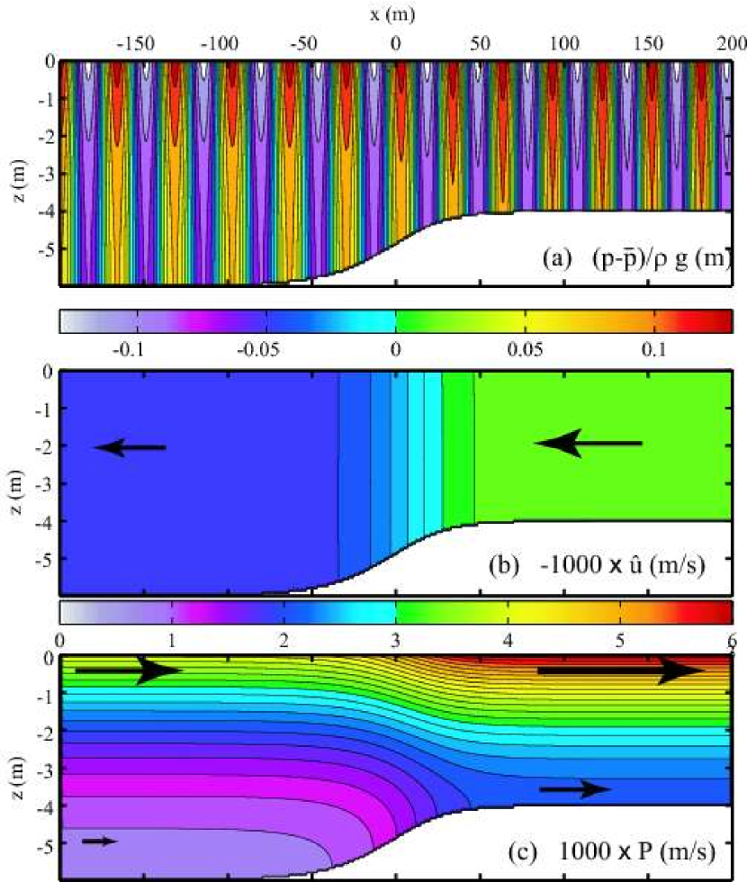
Figure 2: (a) Instantaneous pressure perturbation $(p-\overline{p})/(\rho_{w}g)$ given by the NTUA-nl2 model (Belibassakis and Athanassoulis 2002), including the second order Stokes component in waves with amplitude $a=0.12$ m, over the bottom given by eq. (95). (b) Mean current $-\widehat{u}$, and (c) horizontal wave pseudo-momentum $P_{1}$ estimated from eq. (7), and verified to be equal to the Stokes drift. Arrows indicate the flow directions.

Due to the shoaling of the incident waves, the mass transport induced by the waves increases in shallow water, and thus the mean current must change in the $x$ direction to compensate for the divergence in the wave-induced mass transport. We shall further take a zero-mean surface elevation as $x\rightarrow-\infty$. The second order mean elevation is obtained as a result of the model. We also verified that the vertical wave pseudo-momentum compensates for the divergence of the horizontal component so that in this case for linear waves the wave pseudo-momentum is non-divergent (figure 3).

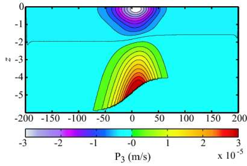
Figure 3: Vertical wave pseudo-momentum for the same case as figure 2, estimated from eq. (7), and verified to satisfy (25).

For mild bottom slopes, the reflection coefficient is small as predicted by Roseau (1976). The NTUA-nl2 model used here generally gives accurate reflection coefficients, but it tends to overestimate very weak reflections. In the first case investigated here, the numerical reflection is $R=1\times 10^{-3}$, with no significant effect on the wave dynamics. The NTUA-nl2 model is used to provide the Fourier amplitudes of the mean, first and second harmonic components of the velocity potential, over a grid of 401 (horizontal) by 101 (vertical) points. From these discretized potential fields, the mean, first and second harmonic velocity components are obtained using second order centered finite differences. As expected, the numerical solution gives a horizontal mean flow $\overline{u}$ that compensates the divergence of the wave mass transport and is thus of order $\sigma/k\varepsilon^{2}$. Further $\overline{u}$ is almost uniform over the vertical and is irrotational (figure 2.b). The vertical mean velocity is of higher order. The GLM momentum balance is thus dominated by the hydrostatic and dynamic pressure terms $p^{H}$ and $S^{\mathrm{J}}$. Although these two terms are individually of the order of $0.01$ m² s^-2, their sum is less than $2\times 10^{-16}$ m² s^-2 in the entire domain, at the roundoff error level. It thus appears that this part of the momentum balance is much more accurate than expected from the asymptotic expansion. Indeed, for any bottom slope, in the limit of small surface slopes and for irrotational flow and periodic waves, the Stokes correction (5) for the pressure and the time average of the Bernoulli equation give the following expression for the modified kinematic pressure (38)

$$\widehat{p}=\frac{\overline{p}^{L}}{\rho_{w}}-\frac{\overline{u^{l}_{j}u^{l}_{j}}}{2} = \frac{\overline{p}}{\rho_{w}}+\frac{1}{\rho_{w}}\overline{\xi_{j}\frac{\partial\widetilde{p}}{\partial x_{j}}}-\frac{\overline{\widetilde{u}_{j}\widetilde{u}_{j}}}{2}$$ (96)

$$= -gz+\frac{1}{\rho_{w}}\overline{\xi_{j}\frac{\partial\widetilde{p}}{\partial x_{j}}}-\overline{\widetilde{u}_{j}\widetilde{u}_{j}}=-gz-\overline{\xi_{j}\frac{\partial^{2}\widetilde{\phi}}{\partial x_{j}\partial t}}-\overline{\frac{\partial\widetilde{\xi_{j}}}{\partial t}\frac{\partial\widetilde{\phi}}{\partial x_{j}}}$$

$$= -gz-\frac{\partial}{\partial t}\overline{\xi_{j}\widetilde{u}_{j}}=-gz$$

where the equalities only hold to second order in the surface slope. Thus the kinematic modified pressure $\widehat{p}$ has no dynamical effect to second order in the wave slope, as already discussed by McWilliams et al. (2004) and Lane et al. (2007). For irrotational flow, this remains true for any bottom topography and even for rapidly varying wave amplitudes, including variations on scales shorter than the wavelength.

Thus the only wave effect is the static change in mean water level (set-up or set-down), and dynamic consequences in the WBBL, where $S^{\mathrm{J}}$ goes to zero, leaving the hydrostatic pressure gradient to drive a mean flow that can only be balanced by bottom friction. For slowly varying wave amplitudes the mean sea level is given by Longuet-Higgins (1967, eq. F1)

$$\overline{\zeta}(x)=-\frac{kE}{\sinh(2kD)}+\frac{k_{0}E_{0}}{\sinh(2k_{0})}$$ (97)

where the $0$ subscript correspond to quantities evaluated at any fixed horizontal position, the choice of which being irrelevant to the estimation of horizontal gradients of $\overline{\zeta}$.

Equation (97) is well verified by the NTUA-nl2 result for the case considered so far (figure 4.a). However, this is no longueur true for rapid variations in the wave amplitude $a(x)$, i.e. due to partially standing waves. In that case one should use Longuet-Higgins’ eq. D (op. cit.)

$$\overline{\zeta}(x)=-\left[\frac{\overline{\widetilde{u}_{\beta}\widetilde{u}_{\beta}-\widetilde{u}_{3}^{2}}}{2g}\right]_{z=0}+\left[\frac{\overline{\widetilde{u}_{\beta}\widetilde{u}_{\beta}-\widetilde{u}_{3}^{2}}}{2g}\right]_{z=0,x=x_{0}},$$ (98)

with $\widetilde{u}_{\beta}$ and $\widetilde{u}_{3}$ given by linear wave theory. Eq. (98) is a generalization of Miche’s (1944a) mean sea level solution under standing waves. Contrary to propagating wave groups, for which the mean sea level is depressed under large waves, here the depression occurs at the nodes of the standing wave, where the horizontal velocities are largest and amplitudes are smallest (figure 4.c).

Eq. (98) is well verified in the presence of partially standing waves. To illustrate this, we have modified the bottom topography, adding a sinusoidal bottom perturbation for $x>180$ m with an amplitude of 5 cm and a bottom wavelength half of the local waves’ wavelength, which maximizes wave reflection (Kreisel 1949). This yields a wave amplitude reflection $R=0.03$, for $\omega=1.2$ rad s^-1, of the order of observed wave reflections over gently sloping beaches (e.g. Elgar et al. 1994). The bottom is shown on figure 4.b. Although the standing wave pattern is hardly noticeable in the surface elevation (the amplitude modulation is only 6%, figure 4.c), the small pressure modulation occur at much smaller scales, so that the associated gradient can overcome the large scale gradients of the hydrostatic pressure (figure 4.d). As a result small partial stading waves can dominating the momentum balance in the WBBL (see Longuet-Higgins 1953, Yu and Mei 2000 for solutions obtained with constant viscosity).

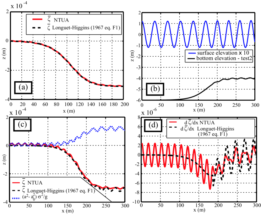
Figure 4: (a) Mean sea level obtained with the NTUA-nl2 model (Belibassakis and Athanassoulis 2002) and the theory of Longuet-Higgins (1967 eq. F1: without standing waves) using conservation of the wave energy flux along the profile. (b) modified bottom profile resulting in a 3% amplitude reflection at $\omega=1.2$ rad s^-1, (c) resulting mean sea level and normalized local wave amplitude $a$, (d) mean sea level gradient (d).

In the presence of such standing waves, and in the absence of strong wave dissipation, the hydrostatic pressure on the scale of the standing waves (e.g. given by Miche 1944a) drives the flow in the WBBL towards the nodes of the standing wave (Longuet-Higgins 1953), and is balanced by bottom friction. This WBBL flow drives an opposite flow above, closing a secondary circulation cell. This secondary circulation is important for nearshore sediment transport just outside of the surf zone (Yu and Mei 2000). If these sub-wavelength circulations are to be modelled, the present $glm2z$-RANS theory should be extended to resolve the momentum balance on the scale of partial standing waves.

This extension is relatively simple as it only introduces additional standing wave terms in all quadratic wave-related quantities, arising from phase-couplings of the incident and reflected waves. This extension provides a generalization of eq. (98) in the presence of other processes. For example, eq. (39) now becomes

$$S^{\mathrm{J}}=g\int_{\mathbf{k_{I}}}\frac{kE({\mathbf{k}})}{\sinh 2kD}\left[\left(1+R^{2}\right)-2R^{2}(\mathbf{k})\cos(2\psi^{\prime}(\mathbf{k}))\right]{\mathrm{d}}{\mathbf{k}}$$ (99)

with $R(\mathbf{k})$ the amplitude reflection coefficient and $2\psi^{\prime}(\mathbf{k})$ is the phase of the partial standing waves defined by $\mbox{\boldmath$\nabla$}\psi^{\prime}=\mathbf{k}$ and $\partial\psi^{\prime}/\partial t=-\mathbf{k}\mbox{\boldmath$\cdot$}\mbox{\boldmath$U$}_{A}t$ such that it is zero at the crest of the incident waves. Note that the integral is over the incident wave numbers only (e.g. for wave propagation directions from 0 to $\pi$). Similar expressions are easily derived for the other wave forcing terms.

4.2 Effects of wave non-linearity

Deep or intermediate water waves do not break very often in most conditions (e.g. Banner et al. 2000, Babanin et al. 2001), thus the particular kinematics of breaking or very steep waves likely contributes little to the average forcing of the current. However, most of the waves break in the surf zone and deviations from Airy wave kinematics may introduce a systematic bias when the $glm2z$-RANS equations are applied in that context. Many wave theories have been developed that are generally more accurate than the Airy wave theory (e.g. Dean 1970). However, they may lack some realistic features found in breaking waves, such as sharp crests. In order to explore the magnitude of this bias, we shall use the kinematics of two-dimensional incipient breaking waves as given by the approximate theory of Miche (1944b).

Miche’s theory is based on the asymptotic expansion of the potential flow from the triangular crest of a steady breaking wave, extending Stokes’ $120^{\circ}$ corner flow to finite depth. From this Miche obtained his criterion for the maximum steepness of a steady breaking wave, i.e. $h/\lambda=0.14\tanh(kh)$ with $h$ the breaking wave height and $\lambda$ the wavelength, which favorably compares with observations. The Miche wave potential $\phi$ and streamfunction $\widetilde{\psi}$ are expressed implicitly as a function $G$ of the coordinates $x-x_{c}+\mathrm{i}(z-z_{c})$, with origin on the wave crest $(x_{c},z_{c})$. The coefficients in the series representing the reciprocal function $G^{\prime}$ are obtained from the boundary condition at the surface and bottom. Unfortunately, these are imposed only under the wave crest and trough, so that the bottom streamline may not be horizontal away from the crest. This is particularly true for small values of $kh$. Due to the expansion of $G^{\prime}$ in powers of $\phi+\mathrm{i}\widetilde{\psi}$, the shape of the wave is nevertheless accurate near the crest, and since the overall drift velocities are dominated by the corner flow near the crest (see also Longuet-Higgins 1979), the approximations of Miche have little consequence on the drift velocities. The function $G^{\prime}$ was modified here to make the bottom actually flat, and the vertical under the trough an equipotential. This deformation adds a weak rotational component to the motion and the wave streamlines are weakly modified at the bottom under the wave trough. The resulting wave for $kh=0.58$ (corresponding to $b=1$ in Miche 1944b) is shown in figure 5.a. A numerical evaluation of that solution is obtained at 201 equally spaced values of $\psi$ and 401 equally spaced values of $\phi$ (figure 5.b). The GLM displacement field $\xi$ is computed as described in section 2.1. Since the streamlines are known in the frame of reference of the wave, Lagrangian positions of 201 particles initially placed below the crest at $x_{i}(0)=0$, were tracked over four Eulerian wave periods. The positions $(x_{i}(t),z_{i}(t))$ are given by the potential $\phi_{i}(t)$ and streamfunction $\psi_{i}$. The Lagrangian period for each particle $T^{L}_{i}$ is determined by detecting the first time when the particles pass under the crest again. The Lagrangian mean velocity of each particle is then $x_{i}(T^{L}_{i})/T^{L}_{i}$, and it corresponds to a vertical position $\overline{z}_{i}=\int_{0}^{T^{L}_{i}}z_{i}(t)\mathrm{d}t$. This defines the Lagrangian mean velocity $\overline{u}^{L}(\overline{z}_{i})$ in GLM coordinates. Following the coordinate transformation in section 2, we further transform the GLM velocity profile to $z$ coordinate (figure 5.c). The resulting profile of $\overline{\mathbf{u}}^{L}$ has a horizontal tangent at $z=0$, as discussed by Miche (1944b).

Contrary to Miche (1944b) who defined the phase speed $C$ of his wave by imposing a zero mass transport, we have defined $C$ so that $\mathbf{P}=\overline{\mathbf{u}}^{L}$ with the pseudo-momentum $\mathbf{P}$ estimated from eq. (7) using finite differences applied to the displacement field. The two profiles of $\mathbf{P}$, estimated from eq. (7), and $\overline{\mathbf{u}}^{L}$, estimated by time integration of particle positions coincide almost perfectly. Thus the estimation of $\mathbf{P}$ provides a practical method for separating the mean current from the wave motion. Starting from any value of $C$, the difference between $\overline{\mathbf{u}}^{L}$ and $\mathbf{P}$ is the mean current velocity $\widehat{\mathbf{u}}$. Here $C$ was corrected to have $\widehat{\mathbf{u}}=0$.

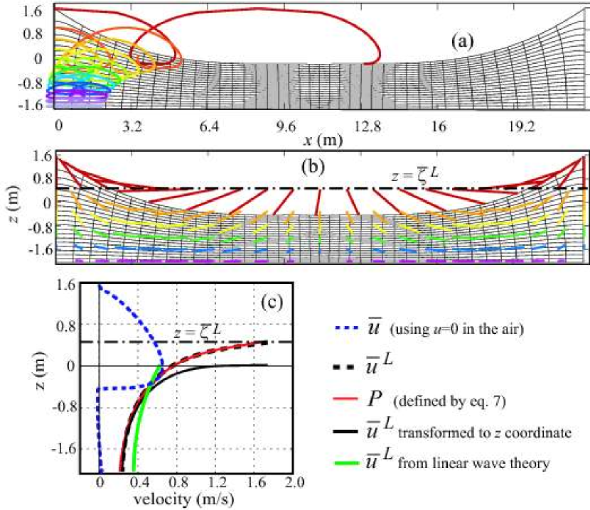
Figure 5: (a) Illustration of the drift over 2 Eulerian periods in periodic Miche waves. Trajectories are color-coded with their initial depth, below a wave crest. The thin black lines are the lines of constant potential and streamfunction at $t=0$. (b) Field of displacements defining the GLM, as in figure 1.c. The dash-dotted line is the GLM position of the free surface $\overline{\zeta}^{L}$. (c) Profiles of Eulerian and Lagrangian mass transport velocity in a Miche wave compared to a linear wave with the same values of $k$ and $h$.

From $\xi$, Bernoulli’s equation can be used to obtain the GLM of velocities and pressure. Compared to linear wave theory, the Stokes drift in a Miche wave is much more sheared. It should be noted that in the cnoidal theory investigated by Wiegel (1959) this drift velocity is depth-uniform. Thus cnoidal wave theories may produce inaccurate results for 3D wave-current interactions when extrapolated to breaking waves. This marked difference in the 3D mean flow forcing due to breaking waves compared to linear waves calls for a deeper investigation of this question. Investigating such kinematics, may provide a rationale for the parameterization of nonlinearity in the $glm2z$-RANS equations proposed here. Such a parameterization is proposed by Rascle and Ardhuin (manuscript in preparation for the Journal of Geophysical Research).

5 Conclusion

We have approximated the exact Generalized Lagrangian Mean (GLM) wave-averaged momentum equations of Andrews and McIntyre (1978a), to second order in the wave slope, allowing for strong and sheared mean currents with limited curvature in the current profile. These approximated equations were then transformed by a change of the vertical coordinate, giving a non-divergent GLM flow in $z$ coordinates. The resulting conservation equations for horizontal momentum (55) and mass (57), with boundary conditions (59)–(74) may be solved using slightly modified versions of existing primitive equations models, forced with the results of spectral wave models. Although the Stokes drift introduces a source of mass at the surface for the quasi-Eulerian flow, this is does not pose any particular problem, and such mass source have long been introduced for the simulation of upwellings. The HYCOM model (Bleck 2002) was modified by R. Baraille to solve a simplified set of the present equations, retaining only the wave-induced mass transport in both the mass and momentum equations, and the tracer equation (in which the advection velocity is simply $\overline{\mathbf{u}}^{L}$, see also MRL04). This work was applied to the a hindcast of the trajectories of sub-surface oil pellets released by the tanker Prestige-Nassau, which sank off Northwest Spain in November 2002 (presentation at the 2004 WMO-JCOMM ‘Oceanops’ conference held in Toulouse, France). The full equations derived here have also been implemented in the ocean circulation model ROMS (Shchepetkin and McWilliams 2003), and results will be reported elsewhere. The equations presented here have also been applied for the modelling of the ocean mixed layer in horizontally-uniform conditions (Rascle et al. 2006).

Although a general expression for the turbulent closure has been given, it has not been made explicit in terms of the wave and mean flow quantities beyond a heuristic closure that combines an eddy viscosity mixing term with the known sources of momentum due to wave dissipation. A proper turbulent closure is left for further work, possibly extending and combining the approaches of Groeneweg and Klopman (1998), with those of Teixeira and Belcher (2002). Further, some wave forcing quantities have been expressed in terms of the Eulerian mean current $\overline{\mathbf{u}}$ instead of the quasi-Eulerian mean current $\widehat{\mathbf{u}}$. The conversion from one to the other, can be done using eq. (24), to the order of approximation used here. However, it would be more appropriate, in particular for large current shears, to start from quasi-Eulerian wave kinematics, instead of Eulerian solutions of the kind given by Kirby and Chen (1989, our eq. 10–12).

Beyond the turbulence closure, there are essentially two practical limitations to the approximate $glm2z$-RANS equations derived here. First, the expansion of wave quantities to second order in the surface slope is only qualitative in the surf zone. Although this was acceptable in two dimensions (see Bowen 1969 and most of the literature on this subject), it is expected to be insufficient in three dimensions due to a significant difference in the profile of the wave-induced drift velocity $\mathbf{P}$, which exhibits a vertical variation with surface values exceeding bottom values by a factor of 3, even for $kh<0.2$ in which case linear wave theory predicts a depth-uniform $\mathbf{P}$. This conclusion is based on both the approximate theory of Miche (1944b), and results of the streamfunction theory of Dalrymple (1974) to 80th order. Such numerical results can be used to provide a parameterization of these effects. Further investigations using more realistic depictions of the kinematics of breaking waves will be needed. Second, the vertical profile of the mean current in the surf zone may be such that the wave kinematics are not well described by the approximations used here. A strong nonlinearity combined with a strong current shear and curvature can lead to markedly different wave kinematics (e.g. da Silva and Peregrine 1988).

With these caveats, the equations derived here provide a generalization of existing equations, extending Smith (2006) to three dimensions and vertically sheared currents, or McWilliams et al. (2004) to strong currents. Of course, mean flow equations can be obtained, at least numerically, using any solution for the wave kinematics with the original exact GLM equations, as illustrated in section 4.2. The wave-forcing on the mean flow is a vortex force plus a modified pressure, a decomposition that allows a clearer understanding of the wave-current interactions, compared to the more traditional radiation stress form. This is most important for the three-dimensional momentum balance and/or in the presence of strong currents, e.g. when a rip current is widened by opposing waves, as observed by Ismail and Wiegel (1983) in the laboratory. Such a situation was also recently modelled by Shi et al. (2006).

Acknowledgments. The correct interpretation of the vertical wave pseudo-momentum $P_{3}$ would not have been possible without the insistent questioning of John Allen. The critiques and comments from Jaak Monbaliu and Rodolfo Bolaños helped correct some misinterpretation of the equations and greatly improved the present paper. N.R. acknowledges the support of a CNRS-DGA doctoral research grant.

Symbol	name	where defined
1 and 2	indices of the horizontal dimensions	after (8)
$3$	index of the vertical dimension	after (8)
$a$	wave amplitude	after (12)
$D=h+\overline{\zeta}$	mean water depth	after (7)
$\mathbf{f}=(f_{1},f_{2},f_{3})$	Coriolis parameter vector (twice the rotation vector)	after (6)
$F_{CC}$, $F_{CS}$, $F_{SC}$ and $F_{SS}$	Vertical profile functions	after (12)
$g$	acceleration due to gravity and Earth rotation	after (7)
$h$	depth of the bottom (bottom elevation is $z=-h$)	before (8)
$J$	Jacobian of GLM average	after (44)
$\mathbf{k}=(k_{1},k_{2})$	wavenumber vector	after (7)
$K_{1}$	Depth-integrated vertical vortex force	(33)
$K_{2}$	Shear-induced correction to Bernoulli head	(29)
$K_{z}$	vertical eddy viscosity	(43)
$(\mbox{\boldmath$\cdot$})^{l}$	Lagrangian perturbation	(2)
$\overline{(\mbox{\boldmath$\cdot$})}^{L}$	Lagrangian mean	(1)
$m$	shear correction parameter	(20)
$\mathbf{M}$	depth-integrated momentum vector	(77)
$\mathbf{M}^{w}$	depth-integrated wave pseudo-momentum vector	(81)
$\mathbf{M}^{m}$	depth-integrated mean flow momentum vector	after (81)
$\mathbf{n}$	unit normal vector	(63)

Table 2: Table of symbols

Symbol	name	where defined
$p$	full dynamic pressure	after (26)
$\widetilde{p}$	wave-induced pressure	(10)
$p^{H}$	hydrostatic pressure	after (35)
$\mathbf{P}=(P_{1},P_{2},P_{3})$	wave pseudo-momentum	(6)
$t$	time	before (1)
$\mathbf{u}=(u_{1},u_{2},u_{3})$	velocity vector
$\widetilde{\mathbf{u}}$	wave-induced velocity	(11) and (68)
$\overline{\mathbf{u}}^{L}$	Lagrangian mean velocity	after (1)
${\mathbf{u}}_{A}$	advection velocity for the wave action	(80)
$\widehat{u}_{\alpha}=\overline{u}^{L}_{\alpha}-P_{\alpha}$	quasi-Eulerian horizontal velocity	before (24)
$s=z+\overline{\xi}_{3}^{L}$	GLM to $z$ transformation function	(48)
$\overline{(\mbox{\boldmath$\cdot$})}^{S}$	Stokes correction	(5)
$S_{ij}$	stress tensor	(62)
$S^{\mathrm{J}}$	wave-induced kinematic pressure	(39)
$S^{\mathrm{Shear}}$	shear-induced correction to $S^{\mathrm{J}}$	(40)
$w=u_{3}$	vertical velocity	before (30)
$\widehat{w}=\overline{u}^{L}_{3}-P_{3}$	quasi-Eulerian vertical velocity	before (30)
$W$	GLM vertical velocity in $z$ coordinates	(54)
$\mathbf{x}=(x_{1},x_{2},x_{3})$	position vector	before (1)

Table 2: Table of symbols, continued

Symbol	name	where defined
$\mathbf{X}$	diabatic source of momentum	after (24)
$\widehat{\mathbf{X}}$	diabatic source of quasi-Eulerian mean momentum	(27)
$z=x_{3}$	vertical position	after (8)
$\alpha$ and $\beta$	dummy indices for horizontal dimensions
$\delta_{ij}$	Kronecker’s symbol, zero unless $i=j$	after (26)
$\varepsilon$	generic small parameter	after (8)
$\varepsilon_{1}$	maximum wave slope	after (7)
$\varepsilon_{2}$	maximum horizontal gradient parameter	after (7)
$\varepsilon_{3}$	maximum current curvature parameter	(9)
$\epsilon_{ijk}A_{j}B_{k}$	component $i$ of the vector product ${\mathbf{A}}\times{\mathbf{B}}$	after (6)
$\zeta$	free surface elevation	before (8)
$\lambda$	wavelength	section 4.2
$\nu$	kinematic viscosity of water	after (62)
$\xi=(\xi_{1},\xi_{2},\xi_{3})$	wave-induced displacement	before (1)
$\rho_{w}$	density of water (constant)	after (12)
$\sigma$	relative radian frequency	after (7)
$\tau_{ij}$	mean stress tensor	(61)
$\psi$	wave phase	after (7)
$\omega$	absolute radian frequency	after (7) and (8)
$\Omega_{3}$	depth-weighted vertical vorticity of the mean flow	(83)
$\nabla$	horizontal gradient operator	after (7)

Table 2: Table of symbols, continued

References

- [Andrews and McIntyre(1978a)] Andrews, D. G., McIntyre, M. E., 1978a. An exact theory of nonlinear waves on a Lagrangian-mean flow. J. Fluid Mech. 89, 609–646.
- [Andrews and McIntyre(1978b)] Andrews, D. G., McIntyre, M. E., 1978b. On wave action and its relatives. J. Fluid Mech. 89, 647–664, corrigendum: vol. 95, p. 796.
- [Ardhuin(2006)] Ardhuin, F., 2006. On the momentum balance in shoaling gravity waves: a commentary of shoaling surface gravity waves cause a force and a torque on the bottom by K. E. Kenyon. Journal of Oceanography 62, 917–922.
- [Ardhuin et al.(2004)Ardhuin, Chapron, and Elfouhaily] Ardhuin, F., Chapron, B., Elfouhaily, T., 2004. Waves and the air-sea momentum budget, implications for ocean circulation modelling. J. Phys. Oceanogr. 34, 1741–1755.
- [Ardhuin et al.(2003)Ardhuin, Herbers, Jessen, and O’Reilly] Ardhuin, F., Herbers, T. H. C., Jessen, P. F., O’Reilly, W. C., 2003. Swell transformation across the continental shelf. part II: validation of a spectral energy balance equation. J. Phys. Oceanogr. 33, 1940–1953.
- [Ardhuin et al.(2007a)Ardhuin, Herbers, Watts, van Vledder, Jensen, and Graber] Ardhuin, F., Herbers, T. H. C., Watts, K. P., van Vledder, G. P., Jensen, R., Graber, H., 2007a. Swell and slanting fetch effects on wind wave growth. J. Phys. Oceanogr. 37 (4), 908–931.
- [Ardhuin and Jenkins(2006)] Ardhuin, F., Jenkins, A. D., 2006. On the interaction of surface waves and upper ocean turbulence. J. Phys. Oceanogr. 36 (3), 551–557.
- [Ardhuin et al.(2007b)Ardhuin, Jenkins, and Belibassakis] Ardhuin, F., Jenkins, A. D., Belibassakis, K., 2007b. Commentary on ‘the three-dimensional current and surface wave equations’ by George Mellor. J. Phys. Oceanogr.Submitted, available at http://arxiv.org/abs/physics/0504097.
- [Ardhuin and Magne(2007)] Ardhuin, F., Magne, R., 2007. Current effects on scattering of surface gravity waves by bottom topography. J. Fluid Mech. 576, 235–264.
- [Babanin et al.(2001)Babanin, Young, and Banner] Babanin, A., Young, I., Banner, M., 2001. Breaking probabilities for dominant surface waves on water of finite depth. J. Geophys. Res. 106 (C6), 11659–11676.
- [Banner et al.(2000)Banner, Babanin, and Young] Banner, M. L., Babanin, A. V., Young, I. R., 2000. Breaking probability for dominant waves on the sea surface. J. Phys. Oceanogr. 30, 3145–3160.
- [Banner and Peirson(1998)] Banner, M. L., Peirson, W. L., 1998. Tangential stress beneath wind-driven air-water interfaces. J. Fluid Mech. 364, 115–145.
- [Battjes(1988)] Battjes, J. A., 1988. Surf-zone dynamics. Annu. Rev. Fluid Mech. 20, 257–293.
- [Belibassakis and Athanassoulis(2002)] Belibassakis, K. A., Athanassoulis, G. A., 2002. Extension of second-order Stokes theory to variable bathymetry. J. Fluid Mech. 464, 35–80.
- [Biesel(1950)] Biesel, F., 1950. Etude théorique de la houle en eau courante. La houille blanche Numéro spécial A, 279–285.
- [Bleck(2002)] Bleck, R., 2002. An oceanic general circulation model framed in hybrid isopicnic-cartesian coordinates. Ocean Modelling 4, 55–88.
- [Bowen(1969)] Bowen, A. J., 1969. The generation of longshore currents on a plane beach. J. Mar. Res. 27, 206–215.
- [Chen et al.(2003)Chen, Kirby, Dalrymple, Shi, and Thornton] Chen, Q., Kirby, J. T., Dalrymple, R. A., Shi, F., Thornton, E. B., 2003. Boussinesq modeling of longshore currents. J. Geophys. Res. 108 (C11), 3362, doi:10.1029/2002JC001308.
- [da Silva and Peregrine(1988)] da Silva, A. F., Peregrine, D. H., 1988. Steep steady surface waves on water of finite depth with constant vorticity. J. Fluid Mech. 195, 281–302.
- [Dalrymple(1974)] Dalrymple, R. A., 1974. A finite amplitude wave on a linear shear current. J. Geophys. Res. 79, 4498–4504.
- [Dean(1970)] Dean, R. G., 1970. Relative validity of water wave theories. J. Waterways, Harbours Div. 96 (WW1), 105–119.
- [Dingemans(1997)] Dingemans, M. W., 1997. Water wave propagation over uneven bottoms. Part 1 linear wave propagation. World Scientific, Singapore, 471 p.
- [Drennan et al.(1999)Drennan, Kahma, and Donelan] Drennan, W. M., Kahma, K., Donelan, M. A., 1999. On momentum flux and velocity spectra over waves. Boundary-Layer Meteorol. 92, 489–515.
- [Elgar et al.(1994)Elgar, Herbers, and Guza] Elgar, S., Herbers, T. H. C., Guza, R. T., 1994. Reflection of ocean surface gravity waves from a natural beach. J. Phys. Oceanogr. 24 (7), 1,503–1,511.
- [Garrett(1976)] Garrett, C., 1976. Generation of Langmuir circulations by surface waves - a feedback mechanism. J. Mar. Res. 34, 117–130.
- [Groeneweg(1999)] Groeneweg, J., 1999. Wave-current interactions in a generalized Lagrangian mean formulation. Ph.D. thesis, Delft University of Technology, The Netherlands.
- [Groeneweg and Battjes(2003)] Groeneweg, J., Battjes, J. A., 2003. Three-dimensional wave effects on a steady current. J. Fluid Mech. 478, 325–343.
- [Groeneweg and Klopman(1998)] Groeneweg, J., Klopman, G., 1998. Changes in the mean velocity profiles in the combined wave-current motion described in GLM formulation. J. Fluid Mech. 370, 271–296.
- [Haas et al.(2003)Haas, Svendsen, Haller, and Zhao] Haas, K. A., Svendsen, I. A., Haller, M. C., Zhao, Q., 2003. Quasi-three-dimensional modeling of rip current systems. J. Geophys. Res. 108 (C7), 3217, doi:10.1029/2002JC001355.
- [Hara and Mei(1987)] Hara, T., Mei, C. C., 1987. Bragg scattering of surface waves by periodic bars: theory and experiment. J. Fluid Mech. 178, 221–241.
- [Herbers et al.(2000)Herbers, Russnogle, and Elgar] Herbers, T. H. C., Russnogle, N. R., Elgar, S., 2000. Spectral energy balance of breaking waves within the surf zone. J. Phys. Oceanogr. 30 (11), 2723–2737.
- [Holm(2002)] Holm, D. D., 2002. Averaged Lagrangians and the mean effects of fluctuations in ideal fluid dynamics. Physica D 179, 253–286.
- [Huang and Mei(2003)] Huang, Z., Mei, C. C., 2003. Effects of surface waves on a turbulent current over a smooth or rough seabed. J. Fluid Mech. 497, 253–287, dOI : 10.1017/S0022112003006657.
- [Ismail and Wiegel(1983)] Ismail, N. M., Wiegel, R. L., 1983. Opposing wave effect on momentum jets spreading rate. J. of Waterway, Port Coast. Ocean Eng. 109, 465–483.
- [Ivonin et al.(2004)Ivonin, Broche, Devenon, and Shrira] Ivonin, D. V., Broche, P., Devenon, J.-L., Shrira, V. I., 2004. Validation of HF radar probing of the vertical shear of surface currents by acoustic Doppler current profiler measurements. J. Geophys. Res. 101, C04003, doi:10.1029/2003JC002025.
- [Janssen(2004)] Janssen, P., 2004. The interaction of ocean waves and wind. Cambridge University Press, Cambridge.
- [Jenkins(1986)] Jenkins, A. D., 1986. A theory for steady and variable wind- and wave-induced currents. J. Phys. Oceanogr. 16, 1370–1377.
- [Jenkins(1987)] Jenkins, A. D., 1987. Wind and wave induced currents in a rotating sea with depth-varying eddy viscosity. J. Phys. Oceanogr. 17, 938–951.
- [Kirby and Chen(1989)] Kirby, J. T., Chen, T.-M., 1989. Surface waves on vertically sheared flows: approximate dispersion relations. J. Geophys. Res. 94 (C1), 1013–1027.
- [Kreisel(1949)] Kreisel, G., 1949. Surface waves. Quart. Journ. Appl. Math. 7, 21–44.
- [Lane et al.(2007)Lane, Restrepo, and McWilliams] Lane, E. M., Restrepo, J. M., McWilliams, J. C., 2007. Wave-current interaction: A comparison of radiation-stress and vortex-force representations. J. Phys. Oceanogr. 37, 1122–1141.
- [Leibovich(1980)] Leibovich, S., 1980. On wave-current interaction theory of Langmuir circulations. J. Fluid Mech. 99, 715–724.
- [Longuet-Higgins(1953)] Longuet-Higgins, M. S., 1953. Mass transport under water waves. Phil. Trans. Roy. Soc. London A 245, 535–581.
- [Longuet-Higgins(1967)] Longuet-Higgins, M. S., 1967. On the wave-induced difference in mean sea level between the two sides of a submerged breakwater. J. Mar. Res. 25, 148–153.
- [Longuet-Higgins(1979)] Longuet-Higgins, M. S., 1979. The trajectories of particles in steep, symmetric gravity waves. J. Fluid Mech. 94, 497–517.
- [Longuet-Higgins(2005)] Longuet-Higgins, M. S., 2005. On wave set-up in shoaling water with a rough sea bed. J. Fluid Mech. 527, 217–234.
- [Lynett and Liu(2004)] Lynett, P., Liu, P. L.-F., 2004. A two-layer approach to wave modelling. Proc. Roy. Soc. Lond. A 460, 2637–2669.
- [Magne et al.(2007)Magne, Belibassakis, Herbers, Ardhuin, O’Reilly, and Rey] Magne, R., Belibassakis, K., Herbers, T. H. C., Ardhuin, F., O’Reilly, W. C., Rey, V., 2007. Evolution of surface gravity waves over a submarine canyon. J. Geophys. Res. 112, C01002.
- [Marin(2004)] Marin, F., 2004. Eddy viscosity and Eulerian drift over rippled beds in waves. Coastal Eng. 50, 139–159.
- [Mathisen and Madsen(1996)] Mathisen, P. P., Madsen, O. S., 1996. Waves and currents over a fixed rippled bed. 1. bottom roughness experienced by waves in the presence and absence of currents. J. Geophys. Res. 101 (C7), 16,533–16,542.
- [Mathisen and Madsen(1999)] Mathisen, P. P., Madsen, O. S., 1999. Wave and currents over a fixed rippled bed. 3. bottom and apparent roughness for spectral waves and currents. J. Geophys. Res. 104 (C8), 18,447–18,461.
- [McIntyre(1988)] McIntyre, M. E., 1988. A note on the divergence effect and the Lagrangian-mean surface elevation in periodic water waves. J. Fluid Mech. 189, 235–242.
- [McWilliams et al.(2004)McWilliams, Restrepo, and Lane] McWilliams, J. C., Restrepo, J. M., Lane, E. M., 2004. An asymptotic theory for the interaction of waves and currents in coastal waters. J. Fluid Mech. 511, 135–178.
- [Mei(1989)] Mei, C. C., 1989. Applied dynamics of ocean surface waves, 2nd Edition. World Scientific, Singapore, 740 p.
- [Mellor(2003)] Mellor, G., 2003. The three-dimensional current and surface wave equations. J. Phys. Oceanogr. 33, 1978–1989, corrigendum, vol. 35, p. 2304, 2005.
- [Miche(1944a)] Miche, A., 1944a. Mouvements ondulatoire de la mer en profondeur croissante ou décroissante. forme limite de la houle lors de son déferlement. application aux digues maritimes. deuxième partie. mouvements ondulatoires périodiques en profondeur régulièrement décroissante. Annales des Ponts et Chaussées Tome 114, 131–164,270–292.
- [Miche(1944b)] Miche, A., 1944b. Mouvements ondulatoire de la mer en profondeur croissante ou décroissante. forme limite de la houle lors de son déferlement. application aux digues maritimes. troisième partie. forme et propriétés des houles limites lors du déferlement. croissance des vitesses vers la rive. Annales des Ponts et Chaussées Tome 114, 369–406.
- [Newberger and Allen(2007)] Newberger, P. A., Allen, J. S., 2007. Forcing a three-dimensional, hydrostatic primitive-equation model for application in the surf zone, part 1: Formulation. J. Geophys. Res.In press.
- [Peregrine(1976)] Peregrine, D. H., 1976. Interaction of water waves and currents. Advances in Applied Mechanics 16, 9–117.
- [Phillips(1977)] Phillips, O. M., 1977. The dynamics of the upper ocean. Cambridge University Press, London, 336 p.
- [Putrevu and Svendsen(1999)] Putrevu, U., Svendsen, I. A., 1999. Three-dimensional dispersion of momentum in wave-induced nearshore currents. Eur. J. Mech. B/Fluids 18, 410–426.
- [Rascle et al.(2006)Rascle, Ardhuin, and Terray] Rascle, N., Ardhuin, F., Terray, E. A., 2006. Drift and mixing under the ocean surface. part 1: a coherent one-dimensional description with application to unstrati.ed conditions. J. Geophys. Res. 111, C03016, doi:10.1029/2005JC003004.
- [Rivero and Arcilla(1995)] Rivero, F. J., Arcilla, A. S., 1995. On the vertical distribution of . Coastal Eng. 25, 135–152.
- [Roseau(1976)] Roseau, M., 1976. Asymptotic wave theory. Elsevier.
- [Russell and Osorio(1958)] Russell, R. C. H., Osorio, J. D. C., 1958. An experimental investigation of drift profiles in a closed channel. In: Proceedings of the 6th International Conference on Coastal Engineering. ASCE, pp. 171–193.
- [Santala and Terray(1992)] Santala, M. J., Terray, E. A., 1992. A technique for making unbiased estimates of current shear from a wave-follower. Deep Sea Res. 39, 607–622.
- [Shchepetkin and McWilliams(2003)] Shchepetkin, A. F., McWilliams, J. C., 2003. A method for computing horizontal pressure-gradient force in an oceanic model with nonaligned vertical coordinate. J. Geophys. Res. 108 (C3), 3090, doi:10.1029/2001JC001047.
- [Shi et al.(2006)Shi, Kirby, and Haas] Shi, F., Kirby, J. T., Haas, K., 2006. Quasi-3d nearshore circulation equations: a cl-vortex force formulation. In: Proceedings of the 30th international conference on coastal engineering, San Diego. ASCE.
- [Smith(2006)] Smith, J. A., 2006. Wave-current interactions in finite-depth. J. Phys. Oceanogr. 36, 1403–1419.
- [Swan et al.(2001)Swan, Cummins, and James] Swan, C., Cummins, I. P., James, R. L., 2001. An experimental study of two-dimensional surface water waves propagating on depth-varying currents. part 1. regular waves. J. Fluid Mech. 428, 273–304.
- [Teixeira and Belcher(2002)] Teixeira, M. A. C., Belcher, S. E., 2002. On the distortion of turbulence by a progressive surface wave. J. Fluid Mech. 458, 229–267.
- [Terray et al.(1996)Terray, Donelan, Agrawal, Drennan, Kahma, Williams, Hwang, and Kitaigorodskii] Terray, E. A., Donelan, M. A., Agrawal, Y. C., Drennan, W. M., Kahma, K. K., Williams, A. J., Hwang, P. A., Kitaigorodskii, S. A., 1996. Estimates of kinetic energy dissipation under breaking waves. J. Phys. Oceanogr. 26, 792–807.
- [Terrile et al.(2006)Terrile, Briganti, Brocchini, and Kirby] Terrile, E., Briganti, R., Brocchini, M., Kirby, J. T., 2006. Topographically-induced enstrophy production/dissipation in coastal models. Phys. of Fluids 18, 126603.
- [Walmsley and Taylor(1996)] Walmsley, J. L., Taylor, P. A., 1996. Boundary-layer flow over topography: impacts of the Askervein study. Boundary-Layer Meteorol. 78, 291–320.
- [Walstra et al.(2001)Walstra, Roelvink, and Groeneweg] Walstra, D. J. R., Roelvink, J., Groeneweg, J., 2001. Calculation of wave-driven currents in a 3D mean flow model. In: Proceedings of the 27th international conference on coastal engineering, Sydney. Vol. 2. ASCE, pp. 1050–1063.
- [Wiegel(1959)] Wiegel, R. L., 1959. A presentation of cnoidal wave theory for practical applications. J. Fluid Mech. 7, 273–286.
- [Xu and Bowen(1994)] Xu, Z., Bowen, A. J., 1994. Wave- and wind-driven flow in water of finite depth. J. Phys. Oceanogr. 24, 1850–1866.
- [Yu and Mei(2000)] Yu, J., Mei, C. C., 2000. Do longshore bars shelter the shore? J. Fluid Mech. 404, 251–268.