Non-Markov Statistical Effects of X-Ray Emission Intensity of The Microquasar Grs 1915+105

R.M. Yulmetyev^1,2, S.A. Demin^1,2, R.M. Khusnutdinov^1,2, O.Yu. Panischev^1,2, P. Hänggi³

¹ Department of Physics, Kazan State University, Kremlevskaya St. 18, Kazan, 420008, RUSSIA
²Department of Physics, Kazan State Pedagogical University, Mezhlauk St. 1, Kazan, 420021, RUSSIA
E-mail: rmy@theory.spu-kazan.ru; sergey@theory.kazan-spu.ru
²Department of Physics, University of Augsburg, Universitätsstrasse 1, D-86135 Augsburg, GERMANY

(Received 22 June 2005)

In this paper we develop the new approach in time series analysis with a variable time step and present the results of quantitative and qualitative estimation of randomness and regularity, and the study of non-Markovian effects of the X-ray emission intensity of the microquasar GRS 1915+105. Our estimation is based on the application of the theory of discrete non-Markovian stochastic processes and gives a wide set of quantitative characteristics and parameters of the studied system with a variable time step. This set reflects the change of the effects of randomness and regularity, the alternation of Markovian and non-Markovian processes in the initial time signals. Initially these characteristics were determined for the simple model systems constructed by means of a molecular dynamics method. Further the calculation of these parameters was executed for the X-ray emission intensity of the microquasar GRS 1915+105. We have developed a theoretical scheme for the detailed analysis of the time series with a variable time step. The new theory allows us to extract more detailed information about the X-ray emission of the microquasar GRS 1915+105 from the experimental time series. The received set of the parameters allows to estimate accurately randomness and stochastic behavior, regularity and robustness, non-Markovian effects of statistical memory in the intensity of the X-ray emission. The analysis of the experimental data with a constant and variable time step is carried out by means of phase portraits, power spectra of the initial time and event correlation function (TCF and ECF), and memory functions (MF) of the junior order, the first three points of non-Markovity parameter.

Key words: discrete non-Markov processes, time series analysis, randomness and non-Markovity, X-ray intensity of GRS 1915+105

PACS numbers: 05.40.Ca; 89.75.-k; 95.75.Wx; 97.80.Jp

1 Introduction

The problems of randomness and stochastic behavior, regularity and robustness have been in the focus of attention in the studies of real complex systems of various nature over the past years. The analysis of individual properties and characteristics of real complex systems is impossible without registration and quantitative estimation of various information on manifestation of chaosity and randomness. By the change of the measure of randomness or regularity it is possible to judge about the complex dynamics of the system and its evolution. The discovery of the phenomenon of chaos in dynamic systems has allowed to take a new look at functioning of complex systems. Chaos is absence of order and it characterizes randomness and unpredictability of changes in the behavior of a system and impossibility to determine their origin and reasons.

While studying multiform manifestations of randomness, the authors have defined chaos, and its the parameters describing chaotic and regular stochastic processes in different ways. As a rule, the search for the most accurate criteria for the estimation of randomness or regularities in the dynamics of real objects is carried out if we have the information on the behavior of the well-known models of nonlinear dynamics such as, for example, Lorentz model, Poisson model etc. Initially for the similar systems one calculates the parameters determining their chaotic dynamics. Further the given parameters are calculates for real physical objects. On the basis of the comparative analysis of these characteristics it is possible to come to certain conclusions about the evolution and further dynamics of the studied system. However the above mentioned models of nonlinear dynamics do not carry sufficient information about the internal properties of real objects. The models similar to real physical objects allow to avoid these defects. The model description of a gas, liquid and solid by the methods of molecular dynamics simulations can serve as an example.

In addition for the estimation of optimal qualitative and quantitative parameters and characteristics of non-Markovian effects and effects of randomness and regularity of X-ray emission intensity dynamics of the microquasar GRS 1915+105 we use the method of molecular dynamics. The galactic microquasar GRS 1915+105 was discovered as an X-ray transient in 1992 [1], and has been observed to be extremely luminous ever since. This binary system contains a 14 $M_{\odot}$ black hole [2] accreting from a late-type giant of mass $0.8\pm 0.5$ $M_{\odot}$ [3] via Roche lobe overflow. GRS 1915+105 is unique among accreting Galactic black holes spending much of its time at super-Eddington luminosities [4]. It is an extremely variable source, exhibiting dramatic, aperiodic variability on a wide range of timescales, from milliseconds to months [5]. GRS 1915+105 is located on the Galactic plane at a distance of $\sim 11-12$ $kpc$ [2, 6] and suffers a large extinction of 25-30 mag in the visual band. The basic characteristics of the GRS 1915+105 binary system is the systemic velocity which is $\gamma=-3\pm 10$ $km/s$, the orbital period of the system is $T_{orb}=33.5\pm 1.5$ days [7]. Spectroscopic observations in the near-infrared H and K bands identified absorption features from the atmosphere of the companion (mass-donating star) in the GRS 1915+105 binary. The detection of ${}^{12}CO$ and ${}^{13}CO$ band heads plus a few metallic absorption lines suggested a $K-M$ spectral type and luminosity class III (giant) [2]. Hard X-ray studies in $20-100keV$ band have shown erratic intensity variations on time scales of days and months [8]-[10]. In Ref. [11] the technique of differentiating and rescaling was applied to the GRS 1915+105 X-ray data. As a result the existence of a fundamental time-scale for the system in the range of 12-17 days was found. In Ref. [12] it was concluded, that microquasar GRS1915+105, as any other black hole system, may be chaotic in nature. One of proofs of the similar behavior of black hole systems is chaotic variability of the X-ray emission [13]. For the estimation of a degree of randomness or regularity of the X-ray emission of the microquasar GRS 1915+105 the correlation dimension of the system [12] is often used.

In this work we present a new method of research of randomness, regularity, robustness and non-Markovian effects in the X-ray emission intensity of the microquasar GRS 1915+105 on the basis of the theory of discrete non-Markovian stochastic processes [14]-[16]. The effects of non-Markovity in real complex systems, natural [14, 15], live [14], [16]-[19], biological [20]-[22] and physical [21, 23] are of special interest for the correlation analysis. This method allows to define the set of characteristics and parameters, which contain detailed information about non-Markovian effects and degrees of randomness of the X-ray emission of the researched system. Initially we have calculated the given characteristics and parameters for model systems by the method of molecular dynamics: for a low density gas with greater randomness and the stochastic behavior in particle motion; for a high density gas; for a liquid near the triple point; for a solid that corresponds to a greater regularity in movement of particles. On the basis of the received results we have executed qualitative and quantitative estimation of non-Markovian effects and of stochastic and regular regimes in the initial signal with a constant and variable time step for the X-ray emission intensity of the microquasar GRS 1915+105.

2 The theoretical framework of the statistical theory of discrete non-Markovian stochastic processes

In this section we present the basic concepts and definitions of the theory of discrete non-Markovian stochastic processes [14]-[16], used here for the analysis of a time series with a constant and variable time step. The theory is constructed on the discrete finite-difference presentation of the Zwanzig-Mori kinetic equations [24, 25] well-known in statistical physics. The theory of the discrete non-Markovian stochastic processes is widely applied to the analysis of real systems of physical, biological, live and social nature [14]-[19],[23]. The dynamic, kinetic and relaxation parameters and characteristics of this theory, contain detailed information about individual properties and qualities of the studied complex system.

2.1 The basic concepts and definitions of the statistical theory of discrete non-Markovian stochastic processes for the analysis of time series with a constant time step

As a rule, the time registration of any characteristics or parameters of a complex system is carried out at discrete time intervals of equal length. It allows to show the essential features of fluctuations and irregularities and also the features of various dynamic regimes in the initial time series. Some key definitions and concepts of the statistical theory of discrete non-Markovian stochastic processes for the analysis of the time series with a constant time step [14]-[16] are given below.

Let us present the time dynamics of the X-ray emission intensity of the microquasar GRS 1915+105 as a discrete time series $x_{j}$ of some variable X:

$$X=\{x(T),x(T+\tau),x(T+2\tau),\ldots,$$ (1)

$$x(T+k\tau),\ldots,x(T+(N-1)\tau)\}.$$

Here $T$ is the initial moment of the time the registration of the X-ray emission intensity, $(N-1)\tau$ is the total time of registration of the signal, $\tau$ is a discretization time step. In the researched time series the discretization time $\Delta t=\tau=1$ day. The mean value of the variable $\langle X\rangle$, fluctuation $\delta x_{j}$, and dispersion $\sigma^{2}$ can be presented as follows:

$$\langle X\rangle=\frac{1}{N}\sum_{j=0}^{N-1}x(T+j\tau),$$ (2)

$$\delta x_{j}=x_{j}-\langle X\rangle,~{}\sigma^{2}=\frac{1}{N}\sum_{j=0}^{N-1}\delta x_{j}^{2}.$$

For the description of the dynamic properties of the studied complex system (the dynamics of correlations) it is convenient to use the normalized time correlation function (TCF):

$$a(t)=\frac{1}{(N-m)\sigma^{2}}\sum_{j=0}^{N-1-m}\delta x(T+j\tau)$$ (3)

$$\times\delta x(T+(j+m)\tau),$$

where $t=m\tau$. Here $\delta x_{j},\delta x_{j+m}$ are fluctuations of the variable $X$ at $j,j+m$ step, correspondingly, $\sigma^{2}$ is an absolute dispersion of the variable $X$. TCF in Eq. (3) satisfies the requirements of normalization and attenuation of correlations:

$$\lim_{t\rightarrow 0}a(t)=1,~{}\lim_{t\rightarrow\infty}a(t)=0.$$ (4)

It is necessary to note, that for a certain class of complex systems the requirement of correlations attenuation is not always possible.

By the use of the Zwanzig-Mori projection operators technique [24, 25] it is possible to receive an interconnected chain of finite-difference equations of a non-Markovian type [14]-[16] for the initial TCF $a(t)$ and the memory function $M_{i}(t)$ ($i=1,2,...,n$):

$$\frac{\Delta a(t)}{\Delta t}=-\tau\Lambda_{1}\sum_{j=0}^{m-1}M_{1}(j\tau)a(t-j\tau)$$

$$+\lambda_{1}a(t),$$

$$\frac{\Delta M_{1}(t)}{\Delta t}=-\tau\Lambda_{2}\sum_{j=0}^{m-1}M_{2}(j\tau)M_{1}(t-j\tau)$$

$$+\lambda_{2}M_{1}(t),$$

$$\ldots,$$

$$\frac{\Delta M_{n-1}(t)}{\Delta t}=-\tau\Lambda_{n}\sum_{j=0}^{m-1}M_{n}(j\tau)M_{n-1}(t-j\tau)$$

$$+\lambda_{n}M_{n-1}(t),$$ (5)

where $\Lambda_{i}$ are relaxation parameters, and parameters $\lambda_{i}$ form the eigenvalue spectrum of Liouville’s quasioperator $\hat{L}$:

$$\lambda_{n}=i\frac{<\textbf{W}_{n-1}\hat{L}\textbf{W}_{n-1}>}{<|\textbf{W}_{n-1}|^{2}>},$$ (6)

$$\Lambda_{n}=i\frac{<\textbf{W}_{n-1}\hat{L}\textbf{W}_{n}>}{<|\textbf{W}_{n-1}|^{2}>}.$$ (7)

Orthogonal dynamic variables $\textbf{W}_{n}$ are received with the help of the Gram-Schmidt orthogonalization procedure:

$$\langle\textbf{W}_{n}\textbf{W}_{m}\rangle=\delta_{n,m}\langle|\textbf{W}_{n}|^{2}\rangle,$$

where $\delta_{n,m}$ is Kronecker’s symbol. To compare the relaxation time scales for the initial TCF $a(t)$ and the $i$th order memory functions $M_{i}(t)$ we use the non-Markovity statistical parameter $\varepsilon$. Initially the given parameter was used for the analysis of the irreversible phenomena in a condensed matter [26]-[29]. According to [14]-[16] we introduce the relaxation times of the initial TCF and the $n$th order memory functions:

$$\tau_{a}=\triangle t\sum_{j=0}^{N-1}a(t_{j}),$$

$$\tau_{M_{1}}=\triangle t\sum_{j=0}^{N-1}M_{1}(t_{j}),$$

$$\ldots,$$

$$\tau_{M_{n}}=\triangle t\sum_{j=0}^{N-1}M_{n}(t_{j}).$$ (8)

Then the spectrum of the non-Markovity parameter is defined as a set of dimensionless quantities [26]:

$$\{\varepsilon_{i}\}=\{\varepsilon_{1},\varepsilon_{2},...,\varepsilon_{n-1}\},$$

$$\varepsilon_{1}=\tau_{a}/\tau_{M_{1}},\varepsilon_{2}=\tau_{M_{1}}/\tau_{M_{2}},\ldots,$$

$$\varepsilon_{n}=\tau_{M_{n-1}}/\tau_{M_{n}}.$$ (9)

Thus, the value $\varepsilon_{n}$ characterizes the comparison of relaxation times of the memory functions $M_{n-1}$ and $M_{n}$. The non-Markovity parameter allows to divide all relaxation processes into Markov, quasi-Markov and non-Markov processes. The spectrum of the non-Markovity parameter defines the stochastic peculiarities of TCF.

In work [14] the concept of the non-Markovity generalized parameter for frequency - dependent case was introduced:

$$\varepsilon_{i}(\nu)=\left\{\frac{\mu_{i-1}(\nu)}{\mu_{i}(\nu)}\right\}^{\frac{1}{2}}.$$ (10)

where $\mu_{i}(\nu)$ is a power spectrum of the $i$th order memory function:

$$\mu_{0}(\nu)=|\triangle t\sum_{j=0}^{N-1}a(t_{j})cos2\pi\nu t_{j}|^{2},$$

$$\ldots,$$

$$\mu_{i}(\nu)=|\triangle t\sum_{j=0}^{N-1}M_{i}(t_{j})cos2\pi\nu t_{j}|^{2}.$$

The above-mentioned equations (3)-(5) present the case of Zwanzig-Mori’s statistical theory [24, 25] for the discrete statistical complex systems. The statistical theory of discrete non-Markovian stochastic processes allows to reveal Markov and non-Markov effects, the effects of statistical memory, effects of a dynamic alternation of stochastic and regular regimes in the initial time series for the X-ray emission intensity of the microquasar GRS 1915+105.

2.2 A new approach to the analysis of discrete time series with a variable time step

In many real complex systems the registration of the initial time signal by different reasons is carried out at time intervals of different length. To such systems we can refer the objects of an astrophysical and seismological nature, some biological and social systems, economic and ecological objects [30, 31, 32].

In the given work we offer a new approach to the description of discrete non-Markovian stochastic processes with a time step of variable length. Such presentation of the initial time signal allows to find the dynamic development of the system, connected with a not real time scale but with its consistent presentation. The basic idea of this method consists in fixing individual events as a sequence of dynamic values. It allows to consider the dynamics of the system as a sequence of individual events. As an example, here we present the analysis of the time registration with a variable time step of the X-ray emission intensity of the microquasar GRS 1915+105.

2.2.1 The basic concepts and definitions of the theory of discrete non-Markovian stochastic processes with a variable time step

Let us consider the chaotic dynamics of the X-ray emission intensity as a sequence of events which are “non-uniform” on a time scale:

$$E=\{\xi_{1},\xi_{2},\xi_{3},\ldots,\xi_{k},\ldots,\xi_{N}\},$$ (11)

where the intervals of time $\Delta t_{ij}=t_{i}-t_{j},j=i+1,j=i-1$, are unequal. Here $\xi_{i}$ presents the event at the moment $t_{i}$ which follows after the event $\xi_{i-1}$, $i=1,...,N$ is the number of the event.

The mean value $\langle E\rangle$, fluctuation $\delta\xi_{i}$, absolute dispersion $\sigma^{2}$ for the set of the random variable $E$ are defined as follows:

$$\langle E\rangle=\frac{1}{N}\sum_{i=1}^{N}\xi_{i},~{}\delta\xi_{i}=\xi_{i}-\langle E\rangle,$$

$$\sigma^{2}=\frac{1}{N}\sum_{i=1}^{N}\delta\xi_{i}^{2}=\frac{1}{N}\sum_{i=1}^{N}\{\xi_{i}-\langle E\rangle\}^{2}.$$ (12)

According to [30]-[32] we shall define the correlation dependence in a sequence of events (11) as follows:

$$a(n)=\frac{1}{(N-m)\sigma^{2}}\sum_{i=1}^{N-m}\delta\xi_{i}\delta\xi_{i+m}.$$ (13)

The function introduced in the similar way $a(t)$ presents the event (not time!) correlation function (ECF). The general requirements suggest, that ECF should have the properties of normalization and attenuation of correlations:

$$\lim_{n\rightarrow 1}a(n)=1,~{}\lim_{n\rightarrow\infty}a(n)=0.$$ (14)

For the description of a discrete sequence of events we shall use Liouville’s finite-difference equation of movement:

$$\frac{\Delta\xi_{i}(n)}{\Delta n}=i\widehat{L}(n,1)\xi_{i}(n),$$ (15)

where $\xi_{i}(n+1)=U(n+1,n)\xi_{i}(n)$, $U(n+1,n)$ is an evolution operator.

Thus, the left hand side of the Eq. (15) can be submitted as follows:

$$\frac{\Delta\xi_{i}}{\Delta n}=U(n+1,n)\xi_{i}(n)-\xi_{i}(n)=$$

$$\{U(n+1,n)-1\}\xi_{i}(n).$$ (16)

Let us present the set of values of the dynamic variable $\delta\xi_{i}$ as a $k$-component vector of the system’s state:
a) the vector of the initial state:

$$\textbf{A}_{k}^{1}=\{\delta\xi_{1},\delta\xi_{2},\delta\xi_{3},...,\delta\xi_{k}\},$$ (17a)

b) the vector of the final state:

$$\textbf{A}_{m+k}^{m}=\{\delta\xi_{m},\delta\xi_{m+1},\delta\xi_{m+2},...,\delta\xi_{m+k}\},$$ (17b)

where $1\leq k\leq N$.

Using the standard expression for the scalar product of vectors and relations (13), (17a) and (17b), we receive the “event” correlation function (ECF) for a stationary sequence of events (11) in the following way:

$$a(n)=\frac{\langle\textbf{A}_{k}^{1}(1)\textbf{A}_{k+m}^{m}(n)\rangle}{\langle|\textbf{A}_{k}^{1}(1)|^{2}\rangle}.$$ (18)

2.2.2 Kinetic equations for discrete non-Markov processes with variable time step

Let us write down the equation of motion (15) for the vector state:

$$\frac{\Delta\textbf{A}_{m+k}^{m}(n)}{\Delta n}=i\widehat{L}(n,1)\textbf{A}_{m+k}^{m}(n).$$ (19)

By the use of the projection operator technique we can split Euclidean vector’s space of state $\textbf{A}(k)$ into two mutually-orthogonal subspaces:

$$\textbf{A}(k)=\textbf{A}^{{}^{\prime}}(k)+\textbf{A}^{{}^{\prime\prime}}(k),$$

$$\textbf{A}^{{}^{\prime}}(k)=\Pi\textbf{A}(k),~{}\textbf{A}^{{}^{\prime\prime}}(k)=P\textbf{A}(k).$$ (20)

Here projector operators $\Pi$ and $P$ have the following properties:

$$\Pi=\frac{|\textbf{A}_{k}^{1}(1)\rangle\langle\textbf{A}_{k}^{1}(1)|}{\langle|\textbf{A}_{k}^{1}(1)|^{2}\rangle},$$

$$P=1-\Pi,~{}\Pi=\Pi^{2},$$

$$P^{2}=P,~{}\Pi P=P\Pi=0.$$ (21)

It allows to split Liouville’s equation (15) into two appropriate equations in two orthogonal subspaces:

$$\frac{\Delta\textbf{A}^{{}^{\prime}}(n)}{\Delta n}=i\widehat{L}_{11}\textbf{A}^{{}^{\prime}}(n)+i\widehat{L}_{12}\textbf{A}^{{}^{\prime\prime}}(n),$$ (22a)

$$\frac{\Delta\textbf{A}^{{}^{\prime\prime}}(n)}{\Delta n}=i\widehat{L}_{21}\textbf{A}^{{}^{\prime}}(n)+i\widehat{L}_{22}\textbf{A}^{{}^{\prime\prime}}(n).$$ (22b)

Here $\widehat{L}_{ij}=\Pi_{i}\widehat{L}\Pi_{j}$ presents the matrix elements of Liouville’s quasioperator $\widehat{L}=\widehat{L}_{11}+\widehat{L}_{12}+\widehat{L}_{21}+\widehat{L}_{22}$. Solving the Eq. (22b) and substituting into the Eq. (22a), we shall receive:

$$\frac{\Delta\textbf{A}^{{}^{\prime}}(n+m)}{\Delta n}=i\widehat{L}_{11}\textbf{A}^{{}^{\prime}}(n+m)$$

$$+i\widehat{L}_{12}\{1+i\Delta n\widehat{L}_{22}\}^{m}\textbf{A}^{{}^{\prime\prime}}(n)$$

$$-\widehat{L}_{12}\sum_{j=1}^{m}\{1+i\Delta n\widehat{L}_{22}\}^{j}\Delta n\widehat{L}_{21}\textbf{A}^{{}^{\prime}}(n+[m-j]).$$ (23)

Acting on the Eq. (23) by the operator of $\langle\textbf{A}(1)|/\langle|\textbf{A}(1)|^{2}\rangle$ and taking into account an idempotentity property of projection operators, we can receive the following finite-difference equation for the initial event correlation function:

$$\frac{\Delta a(n)}{\Delta n}=i\lambda_{1}a(n)-\Delta n\Lambda_{1}\sum_{j=1}^{m}M_{1}(j)a(n-j).$$ (24)

Assuming that $\Delta n=1$, it is possible to formally solve this equation:

$$a(n+1)=\{i\lambda_{1}+1\}a(n)-\Lambda_{1}\sum_{j=1}^{m}M_{1}(j)a(n-j).$$

Here $\lambda_{1}$ is an eigenvalue Liouville’s quasioperator. Relaxation parameter $\Lambda_{1}$ and memory function $M_{1}(j)$ are defined as follows:

$$\lambda_{1}=\frac{\langle\textbf{A}_{k}^{1}(1)\widehat{L}\textbf{A}_{k}^{1}(1)\rangle}{\langle|\textbf{A}_{k}^{1}(1)|^{2}\rangle},$$

$$\Lambda_{1}=\frac{\langle\textbf{A}_{k}^{1}(1)\widehat{L}_{12}\widehat{L}_{21}\textbf{A}_{k}^{1}(1)\rangle}{\langle|\textbf{A}_{k}^{1}(1)|^{2}\rangle},$$

$$M_{1}(j)=\frac{\langle\textbf{A}_{k}^{1}(1)\widehat{L}_{12}\{1+i\Delta n\widehat{L}_{22}\}^{j}\widehat{L}_{21}\textbf{A}_{k}^{1}(1)\rangle}{\langle\textbf{A}_{k}^{1}(1)\widehat{L}_{12}\widehat{L}_{21}\textbf{A}_{k}^{1}(1)\rangle}.$$

Equation (24) contains function $M_{1}(j)$, for which it is possible to repeat the procedure submitted above and receive appropriate finite-difference equations of a non-Markovian type for memory functions of senior orders $n>1$. To simplify the given procedure and generalize the received results one can use Gram-Schmidt orthogonalization procedure [33]:

$$\langle\textbf{W}_{s}\textbf{W}_{p}\rangle=\delta_{s,p}\langle|\textbf{W}_{s}|^{2}\rangle.$$

This operation allows to receive a new vector of state $\textbf{W}_{s}$, contained in the memory function $M_{s}(j)$:

$$\textbf{W}_{0}=\textbf{A}_{k}^{1},~{}\textbf{W}_{1}=\{i\widehat{L}-\lambda_{1}\}\textbf{W}_{0},$$

$$\textbf{W}_{2}=\{i\widehat{L}-\lambda_{2}\}\textbf{W}_{1}-\Lambda_{1}\textbf{W}_{0},\ldots$$ (25)

For new orthogonal dynamic variables $\textbf{W}_{s}$ we receive an interconnected chain of finite-difference equations of a non-Markovian type for the $s$th order normalized correlation functions:

$$\frac{\Delta M_{1}(n)}{\Delta n}=-\Delta n\Lambda_{2}\sum_{j=1}^{m}M_{2}(j)M_{1}(n-j)$$

$$+i\lambda_{2}M_{1}(n),$$

$$\ldots,$$

$$\frac{\Delta M_{s}(n)}{\Delta n}=-\Delta n\Lambda_{s+1}\sum_{j=1}^{m}M_{s+1}(j)M_{s}(n-j)$$

$$+i\lambda_{s+1}M_{s}(n),$$ (26)

where

$$M_{1}(n)=\frac{\langle\textbf{W}_{1}(1)\textbf{W}_{1}(n)\rangle}{\langle|\textbf{W}_{1}(1)|^{2}\rangle},$$

$$\ldots,$$

$$M_{s}(n)=\frac{\langle\textbf{W}_{s}(1)\textbf{W}_{s}(n)\rangle}{\langle|\textbf{W}_{s}(1)|^{2}\rangle},$$

$$\lambda_{s+1}=\frac{\langle\textbf{W}_{s}[i\widehat{L}\textbf{W}_{s}]\rangle}{\langle|\textbf{W}_{s}|^{2}\rangle},$$

$$\ldots,$$

$$\Lambda_{s+1}=\frac{\langle\textbf{W}_{s}[i\widehat{L}\textbf{W}_{s+1}]\rangle}{\langle|\textbf{W}_{s}|^{2}\rangle}.$$ (27)

The frequency - dependence of statistical spectrum of the non-Markovity parameter for the case of time series with a variable time step will be defined as follows:

$$\varepsilon_{i}(\nu)=\left\{\frac{\mu_{i-1}(\nu)}{\mu_{i}(\nu)}\right\}^{\frac{1}{2}},$$ (28)

where $\mu_{i}(\nu)$ is a power spectrum for the $i$th order correlation function:

$$\mu_{1}(\nu)=\left\{\Delta n\sum_{n=1}^{N}M_{1}(n)\cos(2\pi n\nu)\right\}^{2},$$

$$\ldots,$$

$$\mu_{i}(\nu)=\left\{\Delta n\sum_{n=1}^{N}M_{i}(n)\cos(2\pi n\nu)\right\}^{2}.$$ (29)

3 The experimental data and the details of computer simulations

We analyze here two types of the experimental data of the X-ray emission intensity of the microquasar GRS 1915+105 [34]. The first set of the data presents a one-day averaged time series of the X-ray emission intensity in the period from February, 1, 1996 to September, 1, 2004 (a step discretization $\tau=1$ day). For the analysis of the given time series we use the statistical theory of discrete non-Markov processes with a constant time step (see Sect. 2.1).

For the analysis of the non-equidistant time series (the 2nd type of data) we use the statistical theory of discrete non-Markovian stochastic processes with a variable time step (see Sect. 2.2). As experimental data [34] we use the time series of the X-ray emission intensity of the microquasar GRS 1915+105 with a variable time step for the period from February, 1, 1996 to September, 1, 2004. To study the stochastic properties of the X-ray emission we have carried out an additional study of four model systems using the method of molecular dynamics. We have studied a model system (a gas, a liquid, and a solid) consisting of 2048 particles of argon molecules. The particles interacted by Lennard-Jones potential $V(r)=4\varepsilon\{({\sigma}/{r})^{12}-({\sigma}/{r})^{6}\}$ with parameters $\varepsilon/{k_{B}}=120K$ and $\sigma=3.405\textrm{\AA}$ [35]. Here $\varepsilon$ is a well depth, $\sigma$ is a interatomic distance. The simulation was carried out at constant temperature $T^{*}=0.6$ and at various densities $n^{*}=0.1$, $n^{*}=0.5$, $n^{*}=1.0$ and $n^{*}=1.5$. We made use of the “velocity Verlet” algorithm to integrate the equations of motion [36] with a time step $10^{-14}$ sec.

4 Randomness, regularity and non-Markov effects applied to the dynamic analysis of simple model systems and the X-ray emission intensity of the microquasar GRS 1915+105

In this section we present a new method of quantitative estimation of randomness, regularity and non-Markov effects of a time series. Preliminary the calculation of the degree of manifestation of non-Markov effects and randomness or regularities in the dynamic movement of a particle in the given cell will be carried out on simple model systems: a low density gas, a dense gas, a liquid near triple point, a solid. The level of randomness and non-Markov effects is established for each model system and is carried out by means of a set of various characteristics. The set of data of characteristics and quantitative parameters contains reliable information about the degree of randomness or regularity and non-Markov effects in the researched model system. Then on the basis of the calculation of these characteristics we shall proceed to the analysis of a real process: the event variability of the X-ray emission intensity of the microquasar GRS 1915+105.

4.1 Randomness and non-Markov effects in simple model systems

The study of the dynamic features of behavior of real complex systems of a different nature in cardiology, neurophysiology, epidemiology, biophysics, seismology shows the existence of close connection between the first point of the non-Markovity parameter and a quantitative measure of randomness or regularity of the measured signal. To establish this connection we present the results of the study of several simple physical models. The purpose of the similar study consists in detecting typical features of behavior of the non-Markovity parameter for model systems with a different degree of randomness or regularity. The given models were constructed by the method of molecular dynamics. As an example we have considered four Lennard-Jones model systems: a low density gas ($T^{*}=0.6$, $n^{*}=0.1$ in reduced units with parameters, where $\sigma=3.405\textrm{\AA}$ is an interatomic distance, $\varepsilon/k_{B}=120K$ is the well depth; $T=T^{*}\varepsilon/k_{B},n=n^{*}/\sigma^{3}$); a dense gas ($T^{*}=0.6$, $n^{*}=0.5$); a liquid near the triple point ($T^{*}=0.6$, $n^{*}=1.0$) and a solid ($T^{*}=0.6$, $n^{*}=1.5$).

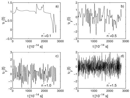
FIG. 1: The time dependence of the $y$–component of particle velocity: a) for a low density gas ($T^{*}=0.6$, $n^{*}=0.1$, in reduced units); b) for a dense gas ($T^{*}=0.6$, $n^{*}=0.5$); c) for a liquid near the triple point ($T^{*}=0.6$, $n^{*}=1.0$); d) for a solid ($T^{*}=0.6$, $n^{*}=1.5$). The weakest correlations correspond to the $y$–component of the particle velocity dynamics for a low density gas. This dynamics characterizes the most chaotic behavior of the particle motion in the studied models. With the increase of density of the model system the correlation in the behavior of particles become more intensive. A model of a solid corresponds to the greatest probability of interaction between particles and the strongest velocity fluctuations.

The time dependencies of the $y$-component velocity for one particle in the studied cell is submitted in Fig. 1. On the basis of the comparative analysis we can reveal a clear distinction between the behavior of particles in each model. For the case of a low density gas (see Fig. 1 ) a weak correlation between the particle velocity and time is observed. It is connected with great (in comparison with the size of particles) distances between particles and the collisionless regime of their behavior. Within a long-time limit weak correlations caused by interaction of two (three) particles are detected. In the given model the most chaotic behavior of a particle in all the studied systems can be observed. Thus, the $y$-component of a particle velocity of a dense gas (see Fig. 1b) differs in strong correlations with time. The interval of fluctuation scattering is relatively fixed. The model shows “moderate chaotization” in the behavior of particles. The following model corresponds to a liquid near the triple point (see Fig. 1c) is characterized by the state of “moderate regularity” in the motion of particles. In comparison with the previous models the correlation between the motion of molecules amplifies noticeably. The amplification of correlations is connected to the increase of the density of the system, accordingly, to greater intensity of interaction of particles. The amplitude of fluctuations is found within a certain interval of values. The obvious regularity in the motion of real molecules corresponds to the model of a solid state (see Fig. 1d). The diagram shows appreciable symmetry of fluctuations regarding the value characterizing the condition of equilibrium in the given model. A high degree of regularity is defined by a high degree of correlation of the states of particles.

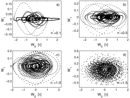
FIG. 2: The phase portraits on a plane projection of the two first orthogonal dynamic variables ($W_{0},W_{1}$) for the considered model systems: a) for a low density gas; b) for a dense gas; c) for a liquid near the triple point; d) for a solid. The structure of phase clouds indicates a level of randomness or regularity of the studied objects. Higher symmetry and regular concentration of phase points concerning the center of coordinates are characteristic for objects with a high degree of regularity. Decreasing of concentration of the phase points near center of coordinates is connected with the increase of the level of randomness in the system behavior.

The phase portraits on plane projections of the two first orthogonal dynamic variables ($W_{0},W_{1}$) are submitted in Fig. 2. Here various degrees of randomness and regularity in the movement of the particles in the system is observed. In all the phase clouds various symmetry is revealed. In case of a low density gas the individual points of the phase portrait generate precise closed structures with a complex chaotic form. In the next models the phase points concentrate near to the center of the coordinate system. The density of the phase cloud grows with the growth of regularity of the model. Concentrated orbits, located around the central nucleus, dissipate. The phase portraits of the solid model are characterized by the greatest concentration of the phase points near the origin of coordinates. It is necessary to note that with the transition of the system from a) to c) the fluctuation scale of variable $W_{2}$ increases. The degree of changes of the orthogonal dynamic variables noticeably differs owing to the difference between the degree of correlations of particles.

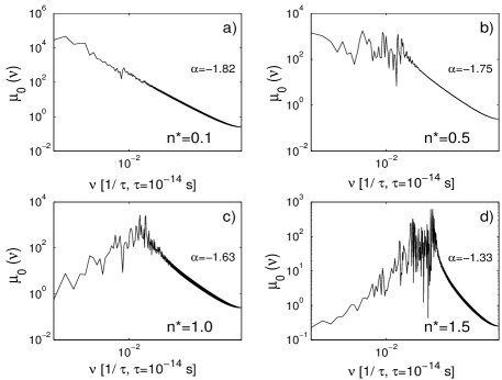
FIG. 3: The power spectrum of the initial time correlation function $\mu_{0}(\nu)$ for four model systems. The parameter $\alpha$ was calculated for each power spectrum. By estimating values $\alpha$ for each model system it is possible to reveal its connection with a level of randomness or regularity in the behavior of the system.

In Fig. 3 the power spectrum of the initial time correlation function $\mu_{0}(\nu)$ for four model systems is submitted. The fractal parameter $\alpha$ of the power spectrum $\mu_{0}(\nu)\sim\nu^{\alpha}$ (where $\alpha<0$ ) was calculated on all frequency scale for all model systems. For a low density gas this parameter amounts to $\alpha=-1.82$; for a gas $\alpha=-1.75$. For a liquid it is equal to $\alpha=-1.63$; for a solid $\alpha=-1.33$. Thus, between the fractal parameter of the power spectrum $\mu_{0}(\nu)$ and the level of manifestation of a randomness and stochastic behavior (the parameter $\alpha$ grows with the increase of a regularity degree) there is appreciable interrelation.

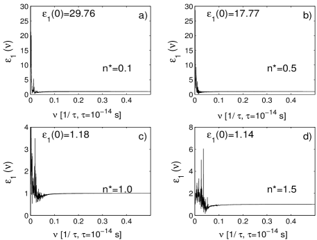
FIG. 4: The frequency dependence of the first point of the non-Markovity parameter $\varepsilon_{1}(\nu)$ for the considered model systems. The analysis of various physical and natural systems specifies a special value of the parameter $\varepsilon_{1}(0)$ in the estimation of level of randomness or regularity. The parameter $\varepsilon_{1}(0)$ make it possible to judge about the level of randomness or regularity in the system. The maximal values of parameter $\varepsilon_{1}(0)$ ($\sim 10^{1}\div 10^{2})$ are characteristic for chaotic and fully randomized processes. Decreasing of the parameter $\varepsilon_{1}(0)$ up to values $\sim 10^{0}$ reflects the increase of level of regularity. It is possible to come to the similar conclusions by estimating the values of this parameter for the submitted models.

In Fig. 4 the frequency dependence of the first point of the non-Markovity parameter (further simply the non-Markovity parameter), calculated by Eq. (10) is submitted.

While analyzing the majority of natural [14, 15] and physical [23] systems earlier we found the following feature in the behavior of the first point of the non-Markovity parameter. The value $\varepsilon_{1}(0)\sim 10^{1}\div 10^{2}$ corresponds to the dynamic states of the systems with the greatest level of randomness and stochastic behavior. For the similar states pronounced Markov effects (manifestation of instantaneous or short-range statistical memory effects) are characteristic. With the increase of regularity and robustness in the system the numerical value of the first point of the non-Markovity parameter on zero frequency decreases up to a unit $\varepsilon_{1}(0)\sim 10^{0}$. Non-Markov processes with amplifying effects of long-range statistical memory correspond to such states.

The analysis of the model systems lead to the similar results. The parameter $\varepsilon_{1}(0)$ for the model of a low density gas (see Fig. 4 ) constitutes 29.76. This is a maximal value of the non-Markovity parameter characterizing a low density gas i.e. the model with the greatest level of randomness and strong Markovian effects. The value of this parameter $\varepsilon_{1}(0)$ for a dense gas equal to 17.77, for a liquid - 1.18, for a solid 1.14. With the increase of the density of the system the numerical value of the non-Markovity parameter on zero frequency decreases to a unit (with the increase of the density of the system the non-Markovian effects increase). This testifies to the possibility to use the non-Markovity parameter as an informational measure of manifestation of randomness and regularity effects.

Thus, the submitted model systems allow to define the set of qualitative and quantitative characteristics for the analysis of a degree of randomness and non-Markov effects in real complex systems. These characteristics carry detailed information about randomness or regularity in the researched system. To these characteristics we can refer: the time correlation in the initial time series, the shape of the phase clouds ($W_{1}=f(W_{0})$), the fractal parameter of the power spectrum $\mu_{0}(\nu)$ and the first point of the non-Markovity parameter on zero frequency $\varepsilon_{1}(0)$. The most authentic and informative parameter of the level of randomness and the manifestation of non-Markov effects is the statistical non-Markovity parameter.

4.2 The analysis of the X-ray emission intensity of the microquasar GRS 1915+105 for the series with a constant time step

The time series of the X-ray emission intensity of the microquasar GRS 1915+105 [34] during the period from February, 1, to September, 1, 2004 (the time discretization is equal to one day) is submitted in Fig. 5. Here we find the presence of quasiperiodic structures which are connected to a relative regularity of the signal within certain time intervals. It the end of the time series the quasiperiodic structures get most noisy therefore their form is destroyed.

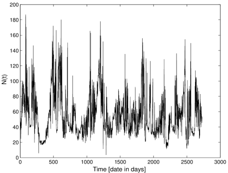
FIG. 5: The time dependence of the X-ray emission intensity of the microquasar GRS 1915+105 with constant time step (step discretization $\tau=1$ day). It is possible to discover quasiperiodic structures in the time dependence. The given structures bring relative regularity in the X-ray emission intensity.

The phase clouds on the plane projections for various combinations of dynamical orthogonal variables $W_{i}$, $W_{j}$ (where $i,j=0..3$) of the X-ray intensity of the microquasar GRS 1915+105 are shown in Fig. 6. It is possible to judge the character of the X-ray emission intensity by the shape of the phase clouds. The phase clouds are of an asymmetric type and consist of a centralized nucleus with a high concentration of phase points and several points surrounding the nucleus.

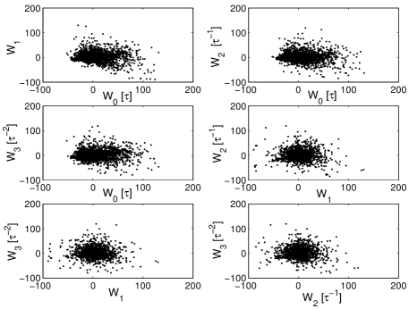
FIG. 6: The phase portraits on the plane projections of the four first dynamic orthogonal variables of the X-ray emission intensity of the microquasar GRS 1915+105 (for time series presented in Fig. 5). The phase clouds consist of the centralized nucleus with a high concentration of phase points and individual points scattered on the perimeter.

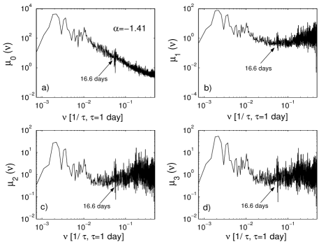
FIG. 7: The power spectrum of the initial TCF $\mu_{0}(\nu)$ (a) and three memory functions of the junior order (b, c, d) for the X-ray emission intensity of the microquasar GRS 1915+105 (for time series presented in Fig. 5). The fractal parameter of the power spectrum $\mu_{0}(\nu)$ is equal to $\alpha=-1.41$. This value is an intermediate value between the similar parameters for the models of a liquid ($\alpha=-1.63$) and a solid ($\alpha=-1.33$).

The power spectrum of the initial TCF $\mu_{0}(\nu)$ (Fig. 7a) and three memory functions of the junior order $\mu_{i}(\nu)$ (where $i=1,2,3$) (Figs. 7b, c, d) for the intensity of the X-ray emission are depicted in Fig. 7. All the figures are submitted on a double logarithmic scale. The fractal parameter of the power spectrum $\mu_{0}(\nu)$ is equal to $\alpha=-1.41$. This value corresponds to the intermediate quantity between the similar parameters for the model of a liquid $\alpha=-1.63$ and a solid $\alpha=-1.33$. In the region of frequencies $\nu$=$5.7\times 10^{-2}\div 7.2\times 10^{-2}f.u.(1f.u.=1/\tau$ where $\tau$ is a discretization time step) a series of dynamic peaks is detected in the power spectra. This frequency range corresponds to a time interval of $\tau=13.8\div 17.4$ days. The maximal peak corresponds to frequency $\nu=6\times 10^{-2}f.u.,$ of $\tau=16.6$ days.

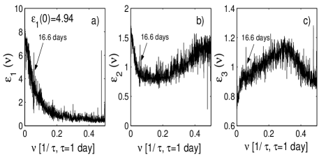
FIG. 8: The frequency dependence of the first three points of the non-Markovity parameter $\varepsilon_{i}(\nu)$ ($i=1,2,3$) for the X-ray emission intensity of the microquasar GRS 1915+105 (for time series presented in Fig. 5). The parameter $\varepsilon_{1}(0)$ plays a special role in the quantification of chaotic and regular processes due to maximal information about the effects of Markovity and non-Markovity, short-range and long-range memory, randomness and regularity effects. For the X-ray emission intensity of the microquasar we have $\varepsilon_{1}(0)=4.94$.

The frequency dependence of the first three points of the non-Markovity parameter $\varepsilon_{i}$, where $i=1,2,3$ for the intensity of the X-ray emission of the microquasar GRS 1915+105 is presented in Fig. 8. Of special value is the first point of the non-Markovity parameter on zero frequency $\varepsilon_{1}(0)=4.94$. This value occupies an intermediate position between the appropriate values for a gas and a liquid. For all the frequency dependencies in the region of frequencies $\nu$=$0.057\div 0.072f.u.$ a series of peaks is detected.

In Table 1 some kinetic ($\lambda_{1},\lambda_{2},\lambda_{3}$) and relaxation parameters ($\Lambda_{1},\Lambda_{2},\Lambda_{3}$) for the X-ray intensity of GRS 1915+105 with a constant time step are submitted. Let us note, that the kinetic parameter $|\lambda_{1}|$ means relaxation rate of the studied system. Small values of kinetic and relaxation parameters signify the manifestation of stochastic effects, randomness and stochastic behavior in the registered time signals of the X-ray emission intensity of the microquasar GRS 1915+105.

Table 1. Some kinetic and relaxation parameters (absolute values) for the X-ray intensity of GRS 1915+105 (constant time step)

$\lambda_{1}~{}[\tau^{-1}]$	$\lambda_{2}~{}[\tau^{-1}]$	$\lambda_{3}~{}[\tau^{-1}]$	$\Lambda_{1}~{}[\tau^{-2}]$	$\Lambda_{2}~{}[\tau^{-2}]$	$\Lambda_{3}~{}[\tau^{-2}]$
0.22	1.20	1.04	0.10	0.10	0.03

4.3 The analysis of the X-ray emission intensity of the microquasar GRS 1915+105 for a time series with a variable step

The initial record of the X-ray emission intensity of the microquasar GRS 1915+105 as a sequence of events is submitted in Fig. 9. The given series essentially differs from the time series with a constant time step (the registration was carried out in the same period) by a visibly big set of the experimental data and consequently is more informative. It allows to define quantitative and qualitative parameters and properties of the studied system with a higher degree of accuracy and reliability.

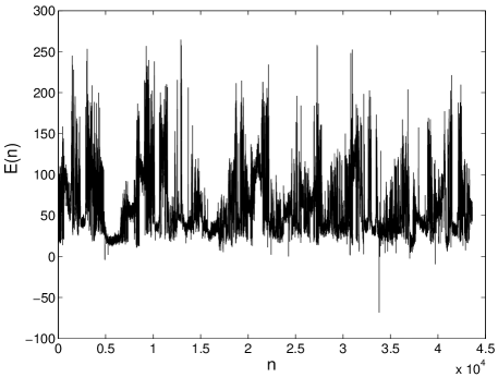
FIG. 9: The discrete sequence of events in the X-ray emission intensity of the microquasar GRS 1915+105 (time series with variable time step, mean time discretization is equal to 96 min). Each point in the given sequence represents a single event of emission.

The power spectra of the initial ECF (Fig. 10 ) and three memory functions of junior orders (Figs. 10b-d) are shown in Fig. 10. All the figures are submitted on a double logarithmic scale. On the whole frequency region of the power spectrum $\mu_{0}(\nu$) strong fractality with the exponent $\alpha=-1.53$ (see Fig. 10a) is observed. Let us note that the fractal parameter for the series with a constant time step corresponds to $\alpha=-1.41$. Hence the initial time signal registered with a variable time step is characterized by greater randomness and stochastic behavior in comparison with a signal with constant time step. Memory functions $\mu_{i}(\nu)$, where $i=1,2,3$ (see Figs. 10b-d) manifest the similar fractal behavior in a wide frequency interval.

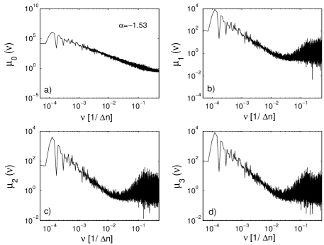
FIG. 10: The power spectrum of the initial correlation function (a) and memory functions of the junior orders (b-d) of the X-ray emission intensity of the microquasar GRS 1915+105 for a non-equidistant time record. The power spectrum of the initial ECF for the event series is characterized by greater fractality than the power spectrum of TCF for the case of a constant time step. In the power spectra of the memory function is observed the peak on frequency $\nu=0.2f.u.$ It reflects also the comparative analysis of the fractal parameter for both cases.

In Fig. 11 the frequency dependencies of first three points of the non-Markovity parameter $\varepsilon_{i}(\nu)$ (where $i=1,2,3$) are submitted. The first point of the non-Markovity parameter $\varepsilon_{1}(\nu)$ in the event presentation (see Fig. 11a) allows to reveal additional features in relaxation processes of the X-ray emission intensity of the microquasar GRS 1915+105. The value of the parameter on zero frequency has increased more than twice and is equal to $\varepsilon_{1}(0)=11.65$. The similar behavior of the non-Markovity parameter (for the series with a variable time step) is connected with the amplification of quasi-Markovian and stochastic effects in the X-ray emission processes. In Fig. 11 markovization effects are observed in frequency behavior $\varepsilon_{1}(\nu)$ as a peak on frequency $\nu=0.238$ $f.u$ (where $1f.u=1/\Delta n$, $\Delta n=$1 event). The values of the two subsequent points of the non-Markovity parameter (see Fig. 11b, c) are close to a unit and are of identical kind for both time series.

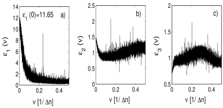
FIG. 11: The frequency dependence of the first three points of the non-Markovity parameter of the X-ray emission intensity of the microquasar GRS 1915+105 for an event correlation function (for series of events presented in Fig. 9). The first point of the non-Markovity parameter $\varepsilon_{1}(\nu)$ (a) is characterized by the following features: the value on zero frequency is equal to $\varepsilon_{1}(0)=11.65$; the peak on frequency $\nu=0.238$ $f.u.$ connected with the sharp amplification of Markovian (stochastic) effects is observed.

In Table 2 some kinetic ($\lambda_{1},\lambda_{2},\lambda_{3}$) and relaxation parameters ($\Lambda_{1},\Lambda_{2},\Lambda_{3}$) for the X-ray intensity of GRS 1915+105 with a variable time step are submitted. The parameter $|\lambda_{1}|$ it is equal to 0.15. Smaller rate of a relaxation for the time series with variable time step is connected to more obvious and more pronounced stochastic behavior. It may be, that the system needs more time for return to a stable state of equilibrium.

Table 2. Some kinetic and relaxation parameters (absolute values) for the X-ray intensity of GRS 1915+105 (variable time step)

$\lambda_{1}~{}[\tau^{-1}]$	$\lambda_{2}~{}[\tau^{-1}]$	$\lambda_{3}~{}[\tau^{-1}]$	$\Lambda_{1}~{}[\tau^{-2}]$	$\Lambda_{2}~{}[\tau^{-2}]$	$\Lambda_{3}~{}[\tau^{-2}]$
0.15	1.16	1.03	0.05	0.12	0.02

Thus, the approach to the description of statistical discrete processes in the event presentation submitted in this work allows to received more detailed and clear picture of the stochastic processes occurring in complex nature systems.

5 Discussion and Conclusion

Energetic and spectral properties, quasi-periodic oscillations (QPO) and the diverse temporal variability of GRS 1915+105 are the focus of numerous studies in last years.

In the paper [37] the problem of the limits concerning the physical information that can be extracted from the analysis of one or more time series typical of astrophysical objects has been considered. The work [38] has clearly established that radio emission from GRS 1915+105 is intimately related to the presence of hard (power-law dominated) intervals in the X-ray light curves. This in turn physically implies a clear relation between a radiatively inefficient flow close to the black hole, and a synchrotron-emitting overflow or jet. This suggest that MHD effects could be responsible for the production and/or confinement of the jets found in system. For the first time in Ref. [39] were observed concurrently in GRS 1915+105 all of the following properties: a strong steady optically thick radio emission corresponding to a powerful compact jet resolved with the VLBA, bright near-IR emission, a strong QPO at $2.5Hz$ in the X-rays and a power law dominated spectrum without any cuttof in the $3-400keV$ range.

J. Rodriguez et al. in the work [40] have presented the results of simulations INTEGRAL and RXTE observations of the microquasar GRS 1915+105. They have focused on the analysis of the unique highly variable observation and have shown that they might have observed a new class of variability. Then they have studied the energetic dependence of a low frequency QPO from steady observations.

A scenario for the variability of the microquasar GRS 1915+105 starts from previous works, leading to the tentative identification of the accretion-ejection instability as the source of the low frequency QPO and other accreting sources [41]. A model for the $\sim 30$ minute cycles often exhibited by GRS 1915+105 is determined by the advection of poloidal magnetic flux to the inner region of the disk, and its destruction by reconnection (leading to relativistic ejections) with the magnetic flux trapped in the vicinity of the central source. This could be extrapolated further to understand the long-term variability of this and other microquasars.

In the paper [42] authors discuss the possible origin of the following behavior: the QPO spectra are well modelled with a cut-off power law except on one occasion where a single power law gives a satisfactory fit (with no cut-off at least up to $\sim 40keV$). The cut-off energy evolves significantly from one observations to the other, from a value of $\sim 21.8keV$ to $\sim 30keV$ in the other observations where it is detected. It was suggested in the work [42] that the compact jet detected in the radio contributes to the hard X-ray ($\geq 20keV$) mostly through synchrotron emission, whereas the X-ray emitted below $20keV$ would originate through inverse Compton scattering. The dependence of the QPO amplitude on the energy can be understood if the modulation of the X-ray flux is contained in the Componized photons and not in the synchrotron ones.

The variability pattern is characterized in Ref. [43] by a pulsing behavior, consisting of a main pulse and a shorter, softer, and smaller amplitude precursor pulse, on a timescale of 5 minutes in the JEM-X $3-35keV$ light curve. It was revealed, that the rising phase is shorter and harder than the declining phase, which is opposite to what has been observed in other otherwise similar variability classes in this source. The fit show the source to be in a soft state characterized by a strong disc component below $\sim 6keV$ and Comptonization by both thermal and non-thermal electrons at higher energies.

The source, which was observed 3 times in the plateau state, before and after a major radio and X-ray flare, showed strong steady optically thick radio emission corresponding to powerful compact jet resolved in the radio emission corresponding to powerful compact jet resolved in the radio images, bright near-infrared emission, a strong QPO at $2.5Hz$ in the X-rays and a powerful law dominated spectrum without cut-off in the $3-300keV$ range [44].

Relativistic jets are now in Ref. [45] believed to be a fairly ubiquitous property of accreting compact objects, and are intimately coupled with the accretion history. Associated with rapid changes in the accretion states of the binary systems, ejections of relativistic plasma can be observed at radio frequencies on timescale of weeks before becoming undetectable. However, recent observations point to long-term effects of these ejecta on the interstellar medium with the formation of large scale relativistic jets around binary systems.

In Ref. [46] authors by Rossi X-ray Timing Explorer have found that as the radio emission becomes brighter and optically thick, the frequency of a ubiquitous $0.5-10Hz$ QPO decreases, the Fourier phase lags between hard ($11.5-60keV$) and soft ($2-4.3keV$) in the frequency range of $0.01-10Hz$ change sign from negative to positive, the coherence between hard and soft photons at low frequencies decreases, and the relativistic amount of low-frequency power in hard photons compared to soft photons decreases.

Energetic dependence of a low frequency QPO in GRS 1915+105 have been analyzed in the work [47]. The results presented could find an explanation in the context of the Accretion-Ejection Instability, which could appear as a rotating spiral or hot point located in the disk, between its innermost edge and the co-rotation radius.

In the present work the dynamic features in the behavior of a particle in the given cell in condensed matter and the X-ray emission intensity of the microquasar GRS 1915+105 were considered jointly on the basis of the statistical theory of non-Markov processes. For this purpose we used two various applications of the submitted theory as it allows to estimate chaotic and regular, random and stochastic, Markov and non-Markov processes defining the dynamics of the studied system. By taking into account the effects of discreteness, long-range and short-range memory, statistical relaxation now we are able to define a set of valuable parameters and characteristics, which contain detailed information about the properties of the studied systems connected with randomness.

On the basis of the comparative analysis of the initial time series, phase portraits, power spectra of the initial TCF and the first point of the non-Markovity parameter we have found some typical features of the behavior of regular and chaotic, Markov and non-Markov components of stochastic processes in studied systems. The systems with high level of chaotization (a low density gas, a dense gas) are characterized by weak correlation between the initial signals, the presence of complex chaotic closed structures in the phase portraits, the high value of the fractal parameter (according to its absolute value) of the power spectrum of TCF and the big value of the first point of the non-Markovity parameter on zero frequency. In the similar systems the effects of short-range or instantaneous statistical memory that correspond to Markovian processes appear. In regular stochastic processes strong correlations in the initial time signals, clear symmetric structures of phase clouds are observed. The last one consists of centralized nucleus of high concentration. Here low values of the fractal parameter (according to its absolute value) of the power spectrum of the initial TCF, small values of the first point of the non-Markovity parameter on zero frequency are observed. In the similar systems the effects of long-range statistical memory can be seen, and relaxation time scales of TCF and memory functions are comparable. The processes describing the given systems are non-Markov ones.

The use of the above submitted technique allows to estimate non-Markov effects, robustness and regularity, stochastic behavior and randomness of the X-ray emission intensity of the microquasar GRS 1915+105 when the initial signal with constant time step is registered. Here the scale of time fluctuations, long-range effects of memory, discreteness of various processes and states, effects of dynamic alternation in the intensity of the X-ray emission play an important role. In the dynamics of the initial time signal of the X-ray emission intensity the fast change of various regimes, sharp and unexpected alternation of various types of fluctuations and correlations were observed. Taking into account discreteness of the experimental data, statistical effects of long-range memory and the constructive role of fluctuations and correlations we have received a detailed information about the properties and parameters which characterize statistical properties of the fluctuating X-ray emission of microquasar GRS 1915+105.

Thus, in this work, a new approach to the description of discrete non-Markov stochastic processes with a variable time step in the event representation is presented. This approach is based on the consecutive use of the idea suggesting the existence of the event correlation functions. The similar correlation functions are new physical quantities determining probabilistic interrelation between a sequence of events. When analyzing the time signal (the X-ray emission intensity of the microquasar GRS 1915+105) with a variable time step the following characteristics were determined: the power spectra of the initial correlation function and memory functions of the junior orders, first three points of the non-Markovity parameter, the fractal parameter of the power spectrum of ECF and the value of the first point of the non-Markovity parameter on zero frequency. These dependencies and parameters allow to receive additional information about the properties and characteristics of the studied system: the quasi-Markov character of relaxation processes in the intensity of the X-ray emission, amplification of Markov effects on certain frequencies, the fractal character of the power spectra of ECF and memory functions.

Finally, this paper only takes the first step in introducing the concept of event correlation analysis of time series and defining it in terms of quantities that can be calculated from an experimental data. We believe, the method developed can form a basis to start formulating further meaningful questions regarding the notions and presentations for real complex systems.

6 Acknowledgments

The authors are grateful to Dr. F.M. Gafarov for the program package and Dr. L.O. Svirina for technical assistance. This work was partially supported by the RFBR (Grants no. 05-02-16639-a), Grant of Federal Agency of Education of Ministry of Education and Science of Russian Federation. This work has been supported in part (P.H.) by the German Research Foundation, SFB-486, project A10.

Bibliography

- [1] A.J. Castro-Tirado, S. Brandt, N. Lundt. IAUC. 2, 5590 (1992).
- [2] J. Greiner, J.G. Cuby, M. J. McCaughrean. Nature. 414, 422 (2001).
- [3] E.T. Harlaftis, J. Greiner. A&A. 414, L13 (2004).
- [4] C. Done, G. Wardzinski, M. Gierlinski. Mon. Not. R. Astron. Soc. 349, 393 (2004).
- [5] M.R. Truss, G.A. Wynn. Mon. Not. R. Astron. Soc. 353, 1048 (2004).
- [6] Ch.R. Kaiser, J.L. Sokolski, K.F. Gunn, C. Brocksopp. arXiv:astro-ph/0409669, (2004).
- [7] J. Greiner. arXiv:astro-ph/0111540, (2001).
- [8] R.S. Foster, E.B. Waltman, M. Tavani, B.A. Harmon, S.N. Zhang, W.S. Paciesas, F.D. Ghigo. ApJ. 467, L81 (1996).
- [9] S.J. Sazonov, A. Eckart, R. Synayaev. Nature. 382, 47 (1996).
- [10] B. Paul, P.C. Agrawal, A.R. Rao, M.N. Vahia, J.S. Yadav, T.M.K. Marar, S. Seetha, K. Kasturirangan. A&A. 320, L37 (1997).
- [11] J. Greenhough, S.C. Chapman, S. Chaty, R.O. Dendy, G. Rowlands. Mon. Not. R. Astron. Soc. 340, 851 (2003).
- [12] B. Mukhopadhyay. arXiv:astro-ph/0402222, (2004).
- [13] S. Nayakshin, S. Rappaport, F. Melia. ApJ. 535, no. 2, 798 (2000).
- [14] R. M. Yulmetyev, P. Hänggi, F. Gafarov. Phys. Rev. E. 62, 6178 (2000).
- [15] R. M. Yulmetyev, F.M. Gafarov, P. Hänggi, R.R. Nigmatullin, Sh. Kayumov. Phys. Rev. E. 64, 066132 (2001).
- [16] R.M. Yulmetyev, P. Hänggi, F. Gafarov. Phys. Rev. E. 65, 046107 (2002).
- [17] R.M. Yulmetyev, S.A. Demin, N.A. Emelyanova, F.M. Gafarov, P. Hänggi. Physica A. 319, 432 (2003).
- [18] R.M. Yulmetyev, N.A. Emelyanova, S.A. Demin, F.M. Gafarov, P. Hänggi, D.G. Yulmetyeva. Physica A. 331, 300 (2004).
- [19] R.M. Yulmetyev, P. Hänggi, F.M. Gafarov. JETP. 123, no. 3, 643 (2003).
-
[20]
I. Goychuk, P. Hänggi. Phys. Rev. E.
61, 4272 (2000);
I. Goychuk, P. Hänggi. Phys. Rev. Lett. 91, 070601 (2003). - [21] L. Gammaitioni, P. Hänggi, P. Jung, F. Marchesoni. Rev. Mod. Phys. 70, 223 (1998).
- [22] J. Timmer, S. Klein. Phys. Rev. E. 55, 3306 (1997).
-
[23]
R.M. Yulmetyev, A.V. Mokshin, P. Hänggi.
Phys. Rev. E. 68, 051201 (2003);
R.M. Yulmetyev, A.V. Mokshin, T. Scopigno, P. Hänggi. J. Phys.: Condens. Matter. 15, 2235 (2003). -
[24]
R. Zwanzig. J. Chem. Phys. 3, 106 (1960);
R. Zwanzig. Phys. Rev. 124, 983 (1961). -
[25]
H. Mori. Prog. Theor. Phys. 33, 423 (1965);
H. Mori. Prog. Theor. Phys. 34, 399 (1965). -
[26]
V.Yu. Shurygin, R.M. Yulmetyev, V.V.
Vorobjev. Phys. Lett. A. 148, 199 (1990);
V.Yu. Shurygin, R.M. Yulmetyev. Phys. Lett. A. 174, 433 (1993);
R.M. Yulmetyev, R.I. Galeev, V.Yu. Shurygin. Phys. Lett. A. 202, 258 (1995). - [27] V.Yu. Shurygin, R.M. Yulmetyev. Zh. Eksp. Teor. Fiz. 99 144 (1991).
- [28] R.M. Yulmetyev, N.R. Khusnutdinov. J. Phys. A. 27 5363 (1994).
-
[29]
R.M. Yulmetyev, V.Yu. Shurygin, T.R. Yulmetyev. Physica
A. 242 509 (1997);
R.M. Yulmetyev, V.Yu. Shurygin, N.R. Khusnutdinov. Acta Phys. Pol. B. 30 881 (1999). - [30] U. Tirnakli, S. Abe. Phys. Rev. E.70, 056120 (2004).
- [31] S. Abe, N. Suzuki. Physica A. 332, 533 (2004).
- [32] S. Abe, N. Suzuki. Physica A. 350, 588 (2005).
- [33] M. Reed, B. Simon. Methods of Modern Mathematical Physics, Volume I: Functional analysis, Academic Press, New York, (1972).
- [34] http://xte.mit.edu/lcextrct/asmsel.html.
- [35] A. Rahman. Phys. Rev. 136, no. 2A, 405 (1964).
- [36] L. Verlet. Phys. Rev. 159, no. 1, 98 (1967).
- [37] R. Vio, N.R. Kristensen, H. Madsen, W. Wamsteker. A&A. 435, 773 (2005).
- [38] M. Klein-Wolt, R.P. Fender, G.G. Pooley, T. Belloni, S. Migliari, E.H. Morgan, M. van der Klis. Mon. Not. R. Astron. Soc. 331, 745 (2005).
- [39] Y. Fuchs, J. Rodriguez, I.F. Mirabel, S. Chaty, M. Ribo, V. Dhawan, P. Goldoni, P. Sizun, G.G. Pooley, A.A. Zdziarski, D.C. Hannikainen, P. Kretschmar, B. Cordier, N. Lund. A&A. 409, L35 (2003).
- [40] J. Rodriguez, D. Hannikainen, O. Vilhu, Y. Fuchs, S.E. Shaw. In “Compact Binaries in the Galaxy and Beyond”, Proc. IUC Colloquim 194 meeting, La Paz, Mexico, Eds. G. Tovmassian, and E. Sion. 20, 28 (2004).
- [41] M. Tagger, R. Varniere, J. Rodriguez, R. Pellat. ApJ. 607, 410 (2004).
- [42] M. Rodriguez, S. Corbel, D.C. Hannikainen, T. Belloni, A. Paizis, O. Vilhu. ApJ. 615, 416 (2004).
- [43] D.C. Hannikainen, J. Rodriguez, O. Vilhu, L. Hjalmarsdotter, A.A. Zdziarski, T. Belloni, J. Poutanen, K. Wu, S.E. Shaw, V. Beckmann, R.W. Hunstead, G.G. Pooley, N.J. Westergaard, I.F. Mirabel, P. Hakala, A. Castro-Tirado, Ph. Durouchoux. A&A. 435, 995 (2005).
- [44] M. Fuchs, J. Rodriguez, S.E. Shaw, P. Kretchmar, M. Ribo, S. Chaty, I.F. Mirabel, V. Dhawan, G.G. Pooley, I. Brown, R. Spencer, D. Hannikainen. arXiv:astro-ph/0404030, (2004).
- [45] S. Corbel. arXiv:astro-ph/0409155, (2004).
- [46] M.P. Muno, R.A. Remillard, E.H. Morgan, E.B. Waltman, V. Dhawan, R.M. Hjellming, G. Pooley. ApJ. 556, 515 (2001).
- [47] J. Rodriguez, Ph. Durouchoux, I.F. Mirabel, Y. Veda, M. Tagger, K. Yamaoka. A&A. 386, 271 (2002).