Electron-ion-ion coincidence experiments for photofragmentation of polyatomic molecules using pulsed electric fields: treatment of random coincidences

Abstract

In molecular photofragmentation processes by soft X-rays, a number of ionic fragments can be produced, each having a different abundance and correlation with the emitted electron kinetic energy. For investigating these fragmentation processes, electron-ion and electron-ion-ion coincidence experiments, in which the kinetic energy of electrons are analyzed using an electrostatic analyzer while the mass of the ions is analyzed using a pulsed electric field, are very powerful. For such measurements, however, the contribution of random coincidences is substantial and affects the data in a non-trivial way. Simple intuitive subtraction methods cannot be applied. In the present paper, we describe these electron-ion and electron-ion-ion coincidence experiments together with a subtraction method for the contribution from random coincidences. We provide a comprehensive set of equations for the data treatment, including equations for the calculation of error-bars. We demonstrate the method by applying it to the fragmentation of free CF₃SF₅ molecules.

1 Introduction

This is probably one of the most boring papers ever published in this journal. There may be no exciting new science in it. However, it will be one of the most useful papers for those readers who are doing or planning to do multi-particle coincidence spectroscopy, because it presents equations in a “ready-to-use” form for the treatment of random coincidences. This problem needs to be solved in order to avoid mistakes in the analysis on multi-particle coincidence data that are recorded in various kinds of fragmentation experiments of polyatomic molecules.

Multi-ion coincidence momentum spectroscopy is often used in molecular photofragmentation studies using synchrotron radiation (SR) [1, 2, 3]. Electron-ion(-ion) coincidence momentum spectroscopy is also widely used in molecular photoionization study [4, 5, 6, 7]. In these measurements, static extraction fields are applied and all the electrons and ions emitted in all directions (4$\pi$ sr) are collected. In such measurements, the random coincidences are minimized by using a sophisticated filtering of the recorded events or very low ionization rates.

For many applications, however, these approaches and tricks can not be used. Filtering criteria based on momentum conservation cannot be used if there are some undetected neutral fragments. This often happens in the reaction pathways for larger molecules. In such cases, the measured data are no longer kinematically complete. Static extraction fields used for the above listed experiments spoil the energy resolution for electrons. Also the measurements are limited to relatively low kinetic energy electrons. If the kinetic energy of the electron is high (say, more than 50 eV), it becomes practically impossible to collect the electrons from 4$\pi$ sr keeping reasonable resolution. If one tries to improve the electron energy resolution, one needs to restrict the acceptance angle of the electrons, keeping the source volume field-free. The experiments can be done, for example, in such a way that the photoelectron emission is observed with limited acceptance angles in certain directions using an electrostatic analyzer or a conventional time-of-flight (TOF) analyzer, whereas the molecular fragments emitted all directions ($4\pi$ sr) are collected using pulsed electric field [8, 9, 10, 11]. In such experiments, the problem of random coincidences becomes non-trivial, especially if one tries to detect two or more ions in coincidence with electrons. Kämmerling and coworkers [12] discussed the problem of a high level of electron-random ion coincidences for the case of multiple photoionization of atoms. They stressed the need for a reference ion measurement using a “random” trigger instead of the electron detection. In a way this paper might be considered a generalization of their formalism for multiple detectors, if the multi-hit capability of the ion detector is formally treated as multiple “yes-no” ion detectors. Because of the presence of different fundamental processes for molecules leading to single ions and multiple ion pairs in the same experiment, the problem is already rather complicated and we decided to partially neglect the dead time effects of the ion detector.

In this paper, we describe how to perform these experiments and how to deal with subtraction of the random coincidences, presenting the method in form of “ready to use” equations. In the following section, we describe an experimental apparatus and procedures that were successfully used for SR experiments as an practical example. All the details of the subtraction of the random coincidences will be given in section 3. In section 4, we present some experimental results as demonstrations for the necessity of the proper subtraction of the random coincidences. Section 5 is a summary.

2 Experiment

2.1 Coincidence setup

Photofragmentation of polyatomic molecules following inner-shell excitation by soft x-rays has been widely studied in the last two decades. Even for small molecules, many different ions and ion pairs can be produced, each stemming from different Auger final states. To disentangle the fragmentation pathways after molecular Auger decay following inner-shell excitation, coincidence measurement between the Auger electron and the fragment ion is indispensable. In order to investigate molecular fragmentation after inner-shell excitation, we developed an Auger-electron–multiple-ion coincidence apparatus, described in detail elsewhere [10, 13]. The apparatus was installed at the c-branch of the high-resolution soft X-ray monochromator [14] in beamline 27SU [15] at SPring-8, an 8 GeV SR facility in Japan: the radiation source is a figure-8 undulator [16].

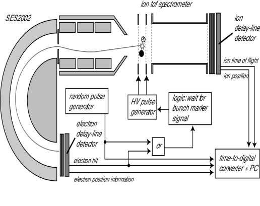
Figure 1: Schematic of the experimental setup and the data acquisition system for synchrotron radiation experiment.

A schematic of our apparatus is shown in Fig. 1. To obtain high resolution for the electron kinetic energy, a dispersive spectrometer with a limited detection angle (Gammadata-Scienta SES2002) is used. An ion TOF spectrometer is placed on the opposite side of the electron spectrometer. The sample gas is introduced as an effusive beam between the pusher and extractor electrodes of the ion spectrometer through a needle. No static extraction field is present in the source region. All voltages of the electron spectrometer are fixed during the coincidence experiment. Electrons pass the pusher electrode, enter the electron spectrometer, and are detected by a fast position resolving detector (Roentdek DLD40). Triggered by the electron detection or a periodic “random” pulse, rectangular high voltages pulses with opposite signs are generated by a pulse generator (GPTA HVC-1000) and applied symmetrically to the pusher and extractor electrodes. The ions are detected by another delay-line detector set (Roentdek DLD80) at the end of the TOF drift tube. All data are recorded by multichannel multi-hit time-to-digital converters (Roentdek TDC-8) and stored in the list mode for off-line analysis. In the list mode, each event consist of one electron or a random pulse followed by zero, one, two, three or four ions.

2.2 Optimum conditions for coincidence experiments

To obtain a reasonable count rate of about 1 Hz a relatively high ionization rate of some KHz is necessary. Under typical experimental conditions, random coincidences including one or two ionic fragments that do not come from the same molecule like the detected electron, are a major contribution to the recorded data. We will only deal with the case were one electron was detected. Due to the limited acceptance angle and the limited energy window of the electron spectrometer electron-electron coincidences are a negligible contribution to the recorded data. The ions that come from the same molecule like the detected electron will be called “true ions” the others will be called “random ions”. There is no such distinction for electrons. There is no way to distinguish between true and random ions for an individual ionization event. The percentage of the contribution of the random ions must be determined in an additional measurement. The problem of a huge contribution of random ions is inherent to the present experiment, as the acceptance angle for the high resolution electron spectrometer is $\sim 0.001\cdot$ 4$\pi$ sr and therefore 999 of 1000 electrons are not detected. The corresponding ions need time to escape from the region seen by the ion spectrometer. A 30 amu ion with a kinetic energy of 0.1 eV takes about 12 $\mu$s to fly 1 cm. So if the double ionization rate via core hole decay is about 40 KHz, there is at average 1 old ion present, producing a huge contribution of random coincidences. On the other hand, the electron count rate is quite low, because the electron spectrometer sees only a limited part of the spectrum. So in this example, an Auger electron count rate of less than 40 Hz would occur. As a rule of thumb, the best compromise between count rate and true-to-random coincides is obtained for 10-30% random coincidences. In this case, the electron count rate is typically less than 10 Hz. For ion pairs, the situation can be even worse. Two ion species can occur with high abundance, but the cross section for the corresponding ion pair production can be low. In such a case, most of the detected ions pairs belong to random coincidences. This illustrates the need for a fully automatic reliable subtraction method for the random coincidence contribution without any adjustable parameters.

2.3 Reference measurement for the random coincidences

A reference measurement for the random coincidences must be performed under exactly the same experimental conditions as the real coincidence measurement. One very convenient method is to use not only the electron trigger to extract the ions, but also a “random” trigger that comes from an external pulse generator. In order to be able to distinguish the two types of triggers, the information about the trigger type must be recorded as well in the list mode file for each event. Under ideal experimental conditions the electron trigger will always lead to the detection of an ion, while the random trigger should never lead to the detection of any ion. Under typical experimental conditions, however, it is already reasonable, if 1000 electron triggers lead to the detection of 400 ions, while 1000 random triggers lead only to the detection of 150 ions. In this case we would assume that about 250 of the ions that were detected after the electron trigger are true, while 150 of these electrons are random. So the contribution of the true coincidences is 62.5% in this case.

The random trigger rate can be set higher than the electron count rate. So the statistical uncertainties of the random contribution are much lower than that of the real signal. Of course the list mode file should not be overloaded by the random events. As a rule of thumb, use 10 time as many random triggers, as real electron triggers.

A synchrotron light source has a repetition rate of several MHz and the time between the light pulses (time window) is not long enough to detect the electron and the ions. Therefore, the HV is only triggered when either an electron is detected or a random pulse is generated by the pulse generator.

Both the true and random ion signals are time-correlated to the synchrotron light. So is the electron trigger. The random trigger is not. This difference may lead to subtle differences between the random contribution in the electron triggered events and the random triggered events. To avoid this difference an electronic trick is used: There is an electronic signal available, that represents the (delayed) time structure of the light source. It will be called the bunch marker. During the measurement the electron and the random trigger signals do not trigger the extraction field immediately, but wait for the bunch marker signal. The phase of the bunch marker signal should be adjusted in a way to minimize the additional delay time after the electron detection. Using this trick, the random events behave perfectly like the electron events, and the contribution of the random ions can be subtracted form the total ion signal with the method described in this paper.

2.4 Experimental methods to minimize the contribution of random coincidences and their limits

Instead of applying sophisticated statistical methods to subtract the contribution of random coincidences, it would be much more elegant and straightforward to eliminate them by a clever experimental design. Two standard techniques exists to minimize the contribution of the random events. We give a brief account of the limits of their applicability and show that for the experimental conditions considered here, contribution of random coincidences cannot be eliminated to a negligible level. The aim of this article is not to replace these methods, but to properly quantify the contribution of the remaining random coincidences. Of course a situation where the random contribution can be neglected never occurs in practice. The reason is very simple: if the contribution of the random coincidences is reduced by a clever design of the experiment from 10% to, say 1%, for a given count rate, this simply means that the light intensity or the gas pressure can be increased by a factor of 10 to improve the count rate and revert to 10% contribution from random coincidences. In other words, an experiment that takes a week with “negligible” random coincidences can be performed in a day if the random coincidences are subtracted properly.

As described above, slow ions with kinetic energies below 0.1 eV can be the main contribution to the random coincidences in some experiments. Even if they are created at a relatively small rate compared to fast ions, the corresponding sharp peaks are clearly seen in the ion time of flight spectra, because they pile up in the source region until they are extracted by the high voltage pulse. For example N₂⁺ with a kinetic energy of 20 meV needs 27$\mu$s to escape from a region with 1 cm radius. When a static extraction field of 2V/cm is applied, the escape time reduces to about 5 $\mu$s. This effect is clearly seen in the ion time of flight spectra, the sharp lines from the slow ions almost disappear. A similar effect can be achieved, by applying a short ($\sim$1$\mu$s) duration HV sweeping pulse every 5$\mu$s. (Of course the electrons detected during the sweeping pulse should be ignored in the data evaluation.) The obvious change in the ion spectrum creates the illusion that one can easily control the level random coincidences by static or pulsed extraction fields. However the contribution of fast false ions is hardly affected at all. The escape time of F⁺ with a kinetic energy of 2 eV is only 2.22 $\mu$s. So the contribution of fake fast F⁺ ions does not change significantly using reasonable static extraction fields or sweeping pulses with a repetition rate lower than 1 MHz. Figure 2 shows two peaks from the ion time of flight spectrum of CH₃F after F 1s ionization. In this case a small penetrating field extracted the slow ions, unfortunately in the direction of the ion detector, leading to flat background in the time of flight spectrum. Nevertheless the sharp peaks of the slow random ions are efficiently removed in this way. Therefore the contribution of the random coincidences to the slow H₂⁺ ions is not very large. In this spectrum the dominating contribution of random ions are fast ions, as can be clearly seen by the double structure of the peaks belonging to the F⁺ ions.

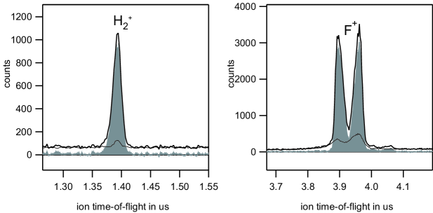
Figure 2: Ion time of flight spectrum including slow H₂⁺ and fast F⁺ ions. Produced upon F 1s ionization of CH₃F. The thick black line is the spectrum produced from all ions triggered by an electron. The thin line is the contribution of the random coincidences derived from the spectrum of ions detected after random triggers. The grey filled graph is the ions spectrum after background subtraction.

Both background suppression methods can only be applied, if the light source used is either continues or has a very high repetition rate, i.e. discharge lamps or synchrotron radiation sources, because they are based on the assumption that most random ions are produced at a different time than the true ions. In experiments with intense pulsed lasers the repetition rate is typically 1 kHz or less and the experimental conditions are often such that more than 10% of the light pulses do ionize at least one molecule. In such a situation 1% of the laser pulses may ionize two or more molecules and the contribution of random coincidences would be about 10%. In this case the random ions are produced during the same laser shot in the same small laser focus as the real ions, so the random ions can not be separated from the real ions using static or pulsed extraction fields.

3 Data evaluation method

3.1 Preparation

3.1.1 The list mode data and filtering

The data is recorded in the list mode. This means that the data structure is a list of events, containing an electron position or a random trigger and 0, 1, 2, 3 or 4 ions. The number 4 is defined by the data acquisition electronics. All ions arriving after the fourth ion will be ignored. Therefore the formulas in this paper which refer to 4-ion events, actually mean 4-or-more-ion events. For electron triggered events any of the ions can come from the same molecule as the electron (true ion) or from another molecule (false ion). There is no way of telling which ion is true and which is false from the data. The number of possible combinations of true and false ions are numerous. We will start the discussion with this event list. Then various numbers and spectra will be defined by evaluating this event list.

The first step of the data evaluation is filtering. This means that the list mode data is changed. Filtering can include the selection of the electron energy, the selection of the ion TOF, the ion emission direction etc. Filtering has two effects. The first effect is the rejection of unwanted events, such as the events for which the electron energy is not in the desired interval. The second effect is a modification of events. For example, if only one ion out of three is in the desired TOF interval, then the event is modified from a one-electron-three-ion event into a one-electron-one-ion event. To avoid confusion, we will only refer to the modified event list after this selection process.

3.1.2 Event statistics

For a given event list, i.e., for a given choice of the TOF interval for the ions and energy interval for the electrons, we can do statistics on the events. We distinguish events with electron triggers and with random triggers. The numbers of these events will be called $N_{e}$ and $N_{RND}$ in the formulas. If more than one electron was detected (or one electron and a random trigger were present), the event is not counted. Since the total number of these events is very small, we do not discuss the systematic effects of this filtering.

The electron trigger can lead to the detection of 0 to 4 ions. The random trigger can also lead to to the detection of 0 to 4 ions. The corresponding probabilities are called $etP_{0,1,2,3,4}$ and $rtP_{0,1,2,3,4}$. (et stands for electron triggered, rt stand for random triggered). These numbers are calculated by counting the number of the events and dividing the result by $N_{e}$ or $N_{RND}$ respectively.

To calculate the random background contribution, we consider the hypothetical probabilities to detect 0, 1, 2, 3 or 4 ions after one electron detection, when the background would be absent. These probabilities are called $TP_{0,1,2,3,4}$ ($T$ stands for true ions). Neglecting the dead time effects of the ion detector, we assume that the chance to detect a random ion is not effected by the presence of the true ion. So the chance to detect 0, 1, 2, 3 or 4 false ions after an electron trigger is also $rtP_{0,1,2,3,4}$.

In order to calculate $TP_{0,1,2,3,4}$ from the known values of $etP_{0,1,2,3,4}$ and $rtP_{0,1,2,3,4}$, we write down a system of linear equations (18), see the appendix. Knowing $rtP_{0,1,2,3,4}$ and $etP_{0,1,2,3,4}$, these equations yield values for $TP_{0,1,2,3,4}$. The numbers $TP_{0,1,2,3,4}$ defined by these equations should all be non-negative and they should add up to 1. Because of statistical errors, some of them may be negative. Therefore the negative values are set to zero and then the numbers $TP_{0,1,2,3,4}$ normalized to sum up as 1. $TP_{0}$ is the probability to find no true ion after the electron detection. There are several possible reasons for this. Most important one is that the detection efficiency of the ion detector is limited. Second, the choice of the TOF region for the ions may not contain all ionic fragments. Furthermore, the electron detector has a certain noise level or dark count rate. So, every ‘electron-trigger’ does not necessarily correspond to the detection of one electron from the source region.

3.1.3 The true number of ionic fragments

To make statements about the real ionization events without the instrumental influences, i.e. the detection efficiency, we define five new values, $P_{0,1,2,3,4}$ that represent the probabilities that 0, 1, 2, 3, 4 ions are present for one electron detected. If the selected TOF region contains all possible ions, $P_{0}$ is the probability for an electron to be detector noise, P₁ the probability be an electron leading to one ion, P₂ the probability be an electron from an ionization leading to two ions etc. Please note that the single and double ionization depend on the charge state of the individual ions. So $P_{1}$ and $P_{2}$ do not exactly belong to single and double ionization processes. To obtain the probabilities for the single and double ionization, one needs to assign the charge state to the detected ions. The value of the ion detection efficiency $PD$ is especially important to compare the yields of doubly charged ions with that of pairs of singly charged ions, because the latter one suffers form the detection efficiency two times. Lets assume that the chosen TOF interval contains all possible ions. Further we assume that the detection efficiency is the same for all ions independent of mass, momentum and charge state. Its value $PD$ is known (determined form an independent measurement). Typically $PD$ should be between 0.2 and 0.4 summarizing the transmission of the grids in the ion spectrometer and the detection efficiency of the detector. So for given values of PD and $TP_{0,1,2,3,4}$ the values of $P_{0,1,2,3,4}$ can be calculated from the set of linear equations (19), given in the appendix.

All values of $P_{0,1,2,3,4}$ must be between 0 and 1. Their sum is 1 by definition. The value of $PD$ can be estimated in a reference measurement where one of the values $P_{1}$ or $P_{2}$ is close to 1. E.g. in the ionization of atoms (e.g. rare gas atoms) , neglecting the detector noise $P_{1}$ is always 1.

If a molecule contains hydrogen, the protons produced are very likely to disobey the approximation that the detection efficiency is the same for all ionic fragments. Their detection efficiency is usually smaller than for the other ions, because protons are usually much faster than the other ions and escape from the region between the pusher and extractor electrodes, before the high voltage pulse is applied.

3.2 Electron spectra

3.2.1 All-electron spectrum

One can make a spectrum of all electrons detected, no matter how many ions where found in coincidence. This is called all-electron-spectrum $AES(x)$. $x$ stands for the kinetic energy of the electron, so technically speaking for a detector position. Because of the discrete nature of the electron detector and the time measurement using a TDC, $AES(x)$ actually means the chance to detect an electron within an interval around the integer value $x$. So there is no need to use the notion of ‘probability density’ for truly continuous spectra. One can create separate electron spectra $ES_{0,1,2,3,4}(x)$ for the events with 0,1,2,3,4 ions, respectively. $AES(x)$ is the sum of all these spectra:

$$AES(x)=ES_{0}(x)+ES_{1}(x)+ES_{2}(x)+ES_{3}(x)+ES_{4}(x)\;.$$ (1)

Without the contribution of the random ions, there would be the hypothetical spectra $HES_{0,1,2,3,4}$(x). The relation between $HES_{0,1,2,3,4}(x)$ and $ES_{0,1,2,3,4}(x)$ is similar to the set of equations 18. One only needs to replace $etP_{0,1,2,3,4}$ by $ES_{0,1,2,3,4}(x)$ and $TP_{0,1,2,3,4}$ by $HES_{0,1,2,3,4}(x)$. Therefore $HES_{0,1,2,3,4}(x)$ can be calculated from $ES_{0,1,2,3,4}(x)$. Solving the equations for $HES_{0,1,2,3,4}(x)$ leads to:

$$HES_{0}(x) = \frac{ES_{0}(x)}{rtP_{0}}$$

$$HES_{1}(x) = \frac{ES_{1}(x)-rtP_{1}\cdot HES_{0}(x)}{rtP_{0}}$$

$$HES_{2}(x) = \frac{ES_{2}(x)-rtP_{2}\cdot HES_{0}(x)-rtP_{1}\cdot HES_{1}(x)}{rtP_{0}}$$

$$HES_{3}(x) = \frac{ES_{3}(x)-rtP_{3}\cdot HES_{0}(x)-rtP_{2}\cdot HES_{1}(x)-rtP_{1}\cdot HES_{2}(x)}{rtP_{0}}$$

The corresponding formula for $HES_{4}$(x) is not written down explicitly, so keep the formulas more readable.

One should remember that $HES_{0,1,2,3,4}(x)$ are defined as what the spectra would look like without the random contribution. The existence of the random contribution redistributes the counts, from the spectra with few ions to the spectra with more ions. Therefore typically the area of $HES_{1}(x)$ contains more counts than that of $ES_{1}(x)$. In order to have an equation of the form true spectrum = measured spectrum - random spectrum, we define the true electron spectra in the following way: $TS_{0}(x)=rtP_{0}\cdot HES_{0}(x),...,TES_{3}(x)=rtP_{0}\cdot HES_{3}(x)$. Then the random backgrounds $BES_{1}(x)$, $BES_{2}(x)$, $BES_{3}(x)$ can be calculated from $ES_{0,1,2,3}(x)$ in the following way:

$$c_{1} = \frac{rtP_{1}}{rtP_{0}},c_{2}=\frac{rtP_{2}}{rtP_{0}}-\frac{rtP_{1}^{2}}{rtP_{0}^{2}}$$

$$c_{3} = \frac{rtP_{3}}{rtP_{0}}+\frac{rtP_{1}^{2}}{rtP_{0}^{2}}-2\cdot\frac{rtP_{1}\cdot rtP_{2}}{rtP_{0}^{2}}$$

$$BES_{1}(x) = c_{1}\cdot ES_{0}(x)$$

$$BES_{2}(x) = c_{2}\cdot ES_{0}(x)+c_{1}\cdot ES_{1}(x)$$

$$BES_{3}(x) = c_{3}\cdot ES_{0}(x)+c_{2}\cdot ES_{1}(x)+c_{1}\cdot ES_{2}(x)$$

$$TES_{0}(x) = ES_{0}(x)$$

$$TES_{1}(x) = ES_{1}(x)-BES_{1}(x)$$

$$TES_{2}(x) = ES_{2}(x)-BES_{2}(x)$$

$$TES_{3}(x) = ES_{3}(x)-BES_{3}(x)$$ (3)

The electron spectrum that belongs to the true e-I coincidences is $TES_{1}(x)$, the electron spectrum that belongs to the true e-I-I coincidences is $TES_{2}(x)$. $TES_{3}(x)$ belongs to the e-I-I-I coincidences. The different terms that contribute to the backgrounds $BES_{2}(x)$ and $BES_{3}(x)$ have a simple interpretation: $c_{2}\cdot ES_{0}(x)$ is the random background of $TES_{2}(x)$ that is caused by two false ions, $c_{1}\cdot ES_{1}(x)$ is the background that is caused by one real and one false ion. $c_{3}\cdot ES_{0}(x)$ is the background in $TES_{3}(x)$ that is caused by three false ions $c_{2}\cdot ES_{1}(x)$ is caused by two false and one real ion, $c_{1}\cdot ES2(x)$ is caused by one false and two real ions. The formulas for the statistical errors of the ture electron spectra $TES_{0,1,2,3}(x)$ are given by the equations 20 in the appendix.

3.2.2 Ion specific electron spectra

For every ion mass to charge ratio, there is a certain small TOF interval called $Iregion(i)$ that contains these ions. One can do the filtering of the event list by restricting the accepted TOF interval of the ions to $Iregion(i)$. The electron spectrum $TES_{1}(x)$ created after this filtering is called the ion specific electron spectrum $TES_{1}I(x,i)$.

3.3 Ion spectra

3.3.1 Ion TOF spectrum and Ion-ion coincidence map

Similar considerations like for the electron spectra are valid for the ion spectra. The simplest quantity to consider is the ion TOF spectrum for all ions detected after an electron trigger $etAI(\hbox{tof})$. (We use “tof” instead of “t” for the time of flight to avoid confusion with “triggered” and “true”).

All ions contribute independent if they are detected alone or as part of a (multiple) ion pair. $tof$ stands for TOF of ion. We will only discuss TOF spectra, but analogous equations are valid for the mass spectra, created by a non-linear transformation of the TOF to the mass/charge ratio. A similar spectrum can be generated for all random triggered ions $rtAI(\hbox{tof})$. Please note that this spectrum does not necessarily represent the true pattern of fragmentation, because the fast ionic fragments are more likely to escape from the region between the pusher and extractor electrode than the slow ones.

Neglecting dead time effects, the detection of one ion is completely independent of the presence of the other ions. Therefore the background subtraction for $etAI(\hbox{tof})$ is very straightforward. The number of electron triggers and random triggers are different. Their ratio will be called scaling factor $SC=N_{e}/N_{RND}$.

$$BetAI(\hbox{tof}) = SC\cdot rtAI(\hbox{tof})$$

$$TetAI(\hbox{tof}) = etAI(\hbox{tof})-BetAI(\hbox{tof})$$

$$\Delta TetAI(\hbox{tof}) = \sqrt{etAI(\hbox{tof})+SC^{2}\cdot rtAI(\hbox{tof})}$$

For the electron-multi ion coincidence technique, the main difference between electron and ion spectra is, that for single ion events we have a TOF or mass spectrum, for double ions events we have a two-dimensional (2D) map, etc. We will only consider the cases for up to two ions. We define $etI(\hbox{tof})$, the spectrum of the ions from single ion events triggered by electron detection and $etII(\hbox{tof1},\hbox{tof2})$, the 2D ion TOF spectrum containing the events with two ions triggered by an electron. The ions are sorted by time of flight, therefore, by definition, we always have the condition $\hbox{tof1}<\hbox{tof2}$. $rtI(\hbox{tof})$ and $rtII(\hbox{tof1},\hbox{tof2})$ are the corresponding spectrum and 2D map for the random triggered events, respectively.

The corresponding spectra of true ions are named $TetI(\hbox{tof})$ and $TetII(\hbox{tof1},\hbox{tof2})$, they are calculated by subtracting the random coincidences $BetI(\hbox{tof})$ and $BetII(\hbox{tof1},\hbox{tof2})$.

$$TetI(\hbox{tof}) = etI(\hbox{tof})-BetI(\hbox{tof})$$

$$TetII(\hbox{tof1},\hbox{tof2}) = etII(\hbox{tof1},\hbox{tof2})-BetII(\hbox{tof1},\hbox{tof2})$$

$$BetI(\hbox{tof}) = SC\cdot TP_{0}\cdot rtI(\hbox{tof})$$

$$BetII(\hbox{tof1},\hbox{tof2}) = SC\cdot TP_{0}\cdot rtII(\hbox{tof1},\hbox{tof2})$$

$$- \frac{2\cdot SC\cdot TP_{0}\cdot rtI(\hbox{tof1})\cdot rtI(\hbox{tof2})}{rtP_{0}\cdot N_{RND}}$$

$$+ \frac{etI(\hbox{tof1})\cdot rtI(\hbox{tof2})+rtI(\hbox{tof1})\cdot etI(\hbox{tof2})}{rtP_{0}\cdot N_{RND}}$$ (5)

The explanation for these formulas is given in in the appendix, see formulas 21 and 22.

3.3.2 Ion pair statistics

For each ion pair $IIpair(j)$ there is a specific region $IIregion(j)$ in the $\hbox{tof1}-\hbox{tof2}$ plane. Because the possible momentum correlation, e.g., emission into opposite directions in a two body fragmentation, these regions are not necessarily chosen rectangular, but rather like tilted ellipses. The number of counts for an ion pair is defined by the ion-ion maps:

$$TCtsIIpair(j) = \sum^{\hbox{tof1},\hbox{tof2}}_{in~{}IIregion(j)}TetII(\hbox{tof1},\hbox{tof2})$$

$$CtsIIpair(j) = \sum^{\hbox{tof1},\hbox{tof2}}_{in~{}IIregion(j)}etII(\hbox{tof1},\hbox{tof2})$$

$$BCtsIIpair(j) = \sum^{\hbox{tof1},\hbox{tof2}}_{in~{}IIregion(j)}BetII(\hbox{tof1},\hbox{tof2})$$

$$TCtsIIpair(j) = CtsIIpair(j)-BCtsIIpair(j)$$ (6)

The last equation is useful to assign error-bars to the number of true ion pairs

$$\Delta TCtsIIpair(j)=\sqrt{CtsIIpair(j)+BCtsIIpair(j)}$$ (7)

For the sake of simplicity, we did not use a proper error propagation formula for $BCtsIIpair(j)$. Instead, we simply considered $\sqrt{BCtsIIpair(j)}$ a good estimate of the statistical uncertainties of $BCtsIIpair(j)$. Strictly speaking, this is an underestimate of the statistical error, if the random background in the single ion spectra $etI(\hbox{tof})$ is large, due to poor experimental conditions. In that case

$$\Delta TCtsIIpair(j)=\sqrt{CtsIIpair(j)+\sqrt{2}\cdot BCtsIIpair(j)}$$ (8)

can be used as an upper limit for $\Delta TCtsIIpair(j)$.

3.4 e-I coincidence diagrams

From the events containing exactly one electron and one ion, three diagrams are created. Two of them have been defined before. An electron spectrum $ES_{1}(x)$ or the true electron spectrum for single ions: $TES_{1}(x)$. The ion spectrum for the single ion events, $etI(\hbox{tof})$ or the true single ion events $TetI(\hbox{tof})$. Now we define a 2D map $etEI(x,\hbox{tof})$ from the electron-ion-events. The total number of the events coincides with the number of counts in $ES_{1}(x)$ and in $etI(\hbox{tof})$. One can check the consistence of the definitions so far, and find that also the number of counts in the true electron spectrum $TES_{1}(x)$ and the true ion spectrum $TetI(\hbox{tof})$ is the same. Now we define the hypothetical quantity $HetEI(x,\hbox{tof})$, the 2D map from the EI events, if there where no random ions. In our formalism ions can be real or false, depending if they belong to the same ion as the electron. According to this definition, the words ‘real’ and ‘false’ cannot be applied to an electron: there are no false electrons. (Detector noise is considered an electron count without real ions.) So, $etEI(x,\hbox{tof})$ contains only two contributions: pairs of electrons and real ions and pairs of electrons and false ions. $HetEI(x,\hbox{tof})$ is related to the measured map $etEI(x,\hbox{tof})$ by:

$$\frac{etEI(x,\hbox{tof})}{N_{e}} = rtP_{0}\cdot\frac{HetEI(x,\hbox{tof})}{N_{e}}+\frac{HES_{0}(x)}{N_{e}}\cdot\frac{rtI(\hbox{tof})}{N_{RND}}$$

$etEI(x,\hbox{tof})/N_{e}$ is the chance to detect an electron with the energy x and and ion with the TOF t. $HetEI(x,\hbox{tof})/N_{e}$ is the chance to detect a real ion with the TOF $tof$ and an electron with the energy $x$. $rtP_{0}$ is the chance to detect no further ion. The second term describes the random contribution. $HES_{0}(x)/N_{e}$ is the chance to detect an electron with the energy $x$ without a real ion. $rtI(\hbox{tof})/N_{RND}$ is the chance to detect a single false ion with the TOF $tof$.

We substitute $HES_{0}(x)=TES_{0}(x)/rtP_{0}=ES_{0}(x)/rtP_{0}$ and define the true electron-ion map as $TetEI(x,\hbox{tof})=rtP_{0}\cdot HetEI(x,\hbox{tof})$

$$etEI(x,\hbox{tof}) = TetEI(x,\hbox{tof})+\frac{ES_{0}(x)\cdot rtI(\hbox{tof})}{rtP_{0}\cdot N_{RND}}$$

and get the random contribution to etEI(x,tof)

$$BetEI(x,\hbox{tof}) = \frac{ES_{0}(x)\cdot rtI(\hbox{tof})}{rtP_{0}\cdot N_{RND}}$$

$$TetEI(x,\hbox{tof}) = etEI(x,\hbox{tof})-BetEI(x,\hbox{tof})$$

The area of $BetEI(x,\hbox{tof})$ coincides with the area of $BES_{1}(x)$ and $BetI(\hbox{tof})$. It is always the number of false e-I coincidences.

3.4.1 A remark about ion specific electron spectra

$TetEI(x,\hbox{tof})$ contains all information about the electrons detected in coincidence with specific ions. So the corresponding ion specific electron spectra $TES_{1}I(x,i)$ could be defined as $\sum^{tof}_{in~{}Iregion(i)}TetEI(x,\hbox{tof})$. This method has a big disadvantage over the method based on filtering the event list, described above. Only the events with exactly one ion contribute to $etEI(x,\hbox{tof})$ – and therefore to $TetEI(x,\hbox{tof})$. So, usually the statistics in $TES_{1}I(x,i)$ get better when $TES_{1}I(x,i)$ is defined as $TES_{1}(x)$ when the time-flight-range of the ions is restricted to $Iregion(i)$ in the filtering of the event file. So the multiple ion events with one ion in the interval $Iregion(i)$ become single ion events and contribute to $TES_{1}I(x,i)$.

3.4.2 Ion-pair specific electron spectra

Now we will discuss how to determine the random background for the spectra of electrons that are coincident with a specific pair of ions. Therefore we formally introduce the 3D map $etEII(x,\hbox{tof1},\hbox{tof2})$ that describes the distribution of the electron–ion-pair events. It is related to $etII(\hbox{tof1},\hbox{tof2})$ and to $ES_{2}(x)$ by:

$$etII(\hbox{tof1},\hbox{tof2}) = \sum_{all~{}x}etEII(x,\hbox{tof1},\hbox{tof2})$$

$$ES_{2}(x) = \sum_{all~{}\hbox{tof1},\hbox{tof2}}etEII(x,\hbox{tof1}\hbox{tof2})$$ (12)

There will be no need to actually create this 3D array $etEII(x,\hbox{tof1},\hbox{tof2})$ in the computer’s memory. The results we will present, only make use of 2D arrays.

The electron spectrum that belongs to a specific ion pair is called $ES_{2}IIpair(x,j)$. It is the histogram of all electrons coincident with two ions in the region $IIregion(j)$.

$$ES_{2}IIpair(x,j) = \sum^{\hbox{tof1},\hbox{tof2}}_{in~{}IIregion(j)}etEII(x,\hbox{tof1},\hbox{tof2})$$ (13)

Lets define the hypothetical 3D spectrum $HetEII(x,\hbox{tof1},\hbox{tof2})$ that would be there without the contribution of the random coincidences. Similar to the considerations for $etII(\hbox{tof1},\hbox{tof2})$ the relations between $HetEII(x,\hbox{tof1},\hbox{tof2})$ and $etEII(x,\hbox{tof1},\hbox{tof2})$ these spectra is:

$$\frac{etEII(x,\hbox{tof1},\hbox{tof2})}{N_{e}} = rtP_{0}\cdot\frac{HetEII(x,\hbox{tof1},\hbox{tof2})}{N_{e}}$$ (14)

$$+ \frac{HetEI(x,\hbox{tof1})}{N_{e}}\cdot\frac{rtI(\hbox{tof2})}{N_{RND}}+\frac{rtI(\hbox{tof1})}{N_{RND}}\cdot\frac{HetEI(x,\hbox{tof2})}{N_{e}}$$

$$+ \frac{rtII(\hbox{tof1},\hbox{tof2})}{N_{RND}}\cdot\frac{HES_{0}(x)}{N_{e}}$$

Meaning that the electron that is detected in coincidence with two ions, can be detected with two true ions, one true and one false ion, one false and one true ion or a pair of false ions. We define the corresponding true electron-ion-ion map $TetEII(x,\hbox{tof1},\hbox{tof2})=rtP_{0}\cdot HetEII(x,\hbox{tof1},\hbox{tof2})$ and get:

$$TetEII(x,\hbox{tof1},\hbox{tof2}) = etEII(x,\hbox{tof1},\hbox{tof2})$$ (15)

$$- \frac{TetEI(x,\hbox{tof1})\cdot rtI(\hbox{tof2})}{rtP_{0}\cdot N_{RND}}-\frac{rtI(\hbox{tof1})\cdot TetEI(x,\hbox{tof2})}{rtP_{0}\cdot N_{RND}}$$

$$- rtII(\hbox{tof1},\hbox{tof2})\cdot\frac{SC}{rtP_{0}}\cdot\frac{ES_{0}(x)}{N_{e}}$$

The true electron spectrum coincident with true ions in the region $IIregion(j)$ is defined by:

$$TES_{2}IIpair(x,j) = \sum^{\hbox{tof1},\hbox{tof2}}_{in~{}IIregion(j)}TtEII(x,\hbox{tof1},\hbox{tof2})$$

So we define the corresponding random background $BS_{2}IIpair(x,j)$:

$$BES_{2}IIpair(x,j) = \sum^{\hbox{tof1},\hbox{tof2}}_{in~{}IIregion(j)}\frac{TetEI(x,\hbox{tof1})\cdot rtI(\hbox{tof2})+rtI(\hbox{tof1})\cdot TetEI(x,\hbox{tof2})}{rtP_{0}\cdot N_{RND}}$$

$$+ \frac{ES_{0}(x)}{N_{e}}\sum^{\hbox{tof1},\hbox{tof2}}_{in~{}IIregion(j)}rtII(\hbox{tof1},\hbox{tof2})\cdot\frac{SC}{rtP_{0}}$$

$$TES_{2}IIpair(x,j) = ES_{2}IIpair(x,j)-BES_{2}IIpair(x,j)$$

$$\Delta TS_{2}IIpair(x,j) = \sqrt{ES_{2}IIpair(x,j)+BES_{2}IIpair(x,j)}$$ (17)

If the summation region $IIregion(j)$ is extended to all ion-ion pairs ($\hbox{tof1}<\hbox{tof2}$) $BES_{2}IIpair(x,j)$ becomes equal to $BES_{2}(x)$.

There is no way to simplify the equation for $BES_{2}IIpair(x,j)$ any further. The summation over all combinations of tof1 and tof2 in the II-region must actually be carried out. This shows that in general the correlation of the true ion and electron (described by $TetEI(x,\hbox{tof})$) and the correlation of two false ions (described by $rtII(\hbox{tof1},\hbox{tof2})$) must be considered for the background subtraction. For the sake of simplicity, in the calculation of $\Delta TS_{2}IIpair(x,j)$ we did not use a proper error propagation formula for $BES_{2}IIpair(x,j)$. We simply considered $\sqrt{BES_{2}IIpair(x,j)}$ a good estimate of the statistical uncertainties of $BES_{2}IIpair(x,j)$. For reasonable experimental conditions, i.e. if the area of TetEI(x,tof) is larger than the area of BetEI(x,tof) in the relevant regions, this is a good estimate.

3.5 Angular distributions, KER spectra

In this paper, we only consider energy spectra of electrons and mass spectra of ions and their correlations. Exactly the same formalism can be applied to distributions with respect to any variable, e.g., emission angles or molecular frame fixed angles, linear momentum, kinetic energy release etc. All of this quantities have to be calculated event by event from the detection positions and the detection times of the particles.

4 Experimental results

As a test for the procedures we analyzed the coincidence data of the molecule SF₅CF₃ taken at a photon energy of 746.95 eV. The chemically shifted F(1s) photo lines where recorded in coincidence with ion pairs. This data set is an ideal test for the methods described here, because F(1s) ionization leads almost inevitably to the production of at least two ions. The molecule does not contain any hydrogen, which usually suffers from low detection efficiency in this type of experiment. Most importantly, the molecule contains only one carbon and one sulfur atom. Therefore a lot of forbidden ion fragment combinations, containing either two carbon or two sulfur atoms appear in the data before the subtraction of the random ion contributions. We know that the contribution from these combinations must be exactly zero after the subtraction of the random coincidences. Figure 3 shows the abundance of the most prominent ion pairs. Among the 42 ion pairs, 16 pairs are forbidden, indicated by the arrows. Without the subtraction of the random contribution (lower panel), some of them e.g. CF⁺-CF₂⁺, CF⁺-CF₃⁺, CF₂⁺-CF₃⁺, and SF⁺-SF₂⁺ have intensities comparable to the dominating allowed peaks. After the subtraction 10 of the 16 forbidden pairs (62 percent) have zero intensity, within a 1 sigma error-bar, and except SF₂⁺-SF₃⁺ (2.5 sigma) all of then are zero within a two sigma error-bars. The error-bars were calculated using equation 7. After the random subtraction no negative intensities occur. So there is also no overestimation of the random background. You can also see, that some of the allowed ions pairs get zero intensity after the subtraction, e.g, SF₂²⁺-CF₃⁺. Without the subtraction of the random background these ion pairs would have been considered real.

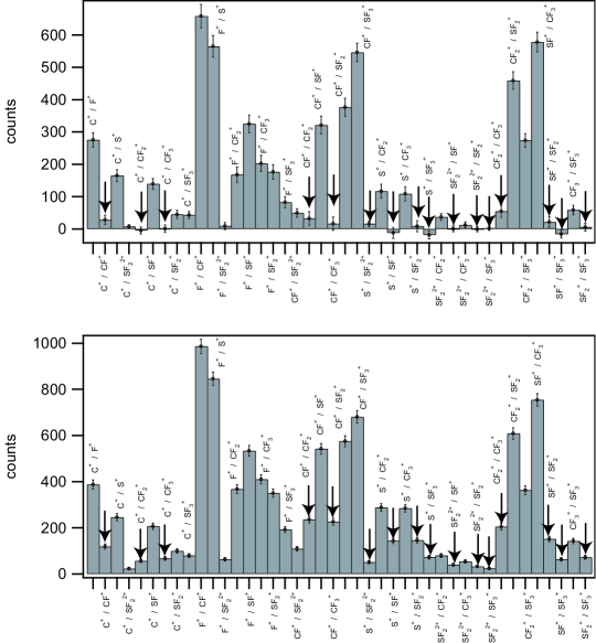
Figure 3: Result of the subtraction for ion pairs. No subtraction lower panel, with subtraction upper panel. The arrows indicate impossible ion combinations.

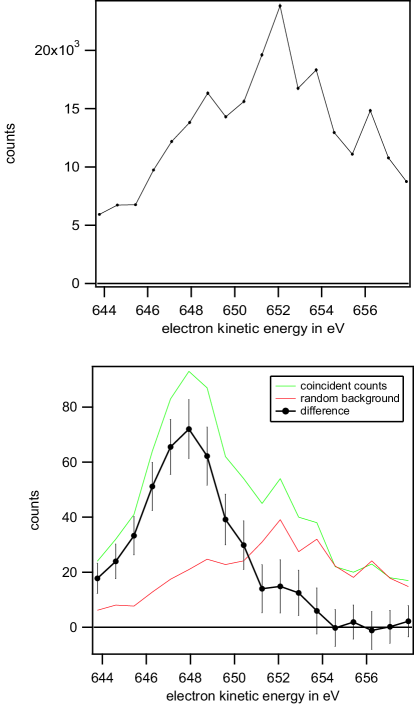
Figure 4: Result of the subtraction for ion pairs in the resonant Auger spectrum at a photon energy of 787.9 eV. Here we have a very low level of ion pair production. Upper panel, total electron spectrum, Lower panel, electrons coincident with ion pairs.

The second test was even more strict. We set the photon energy to 687.9 eV and recorded the resonant Auger electrons in the kinetic energy window from 644 eV to 657 eV. The contribution from ion pairs was very low. Only two ions pairs were found to contribute CF₂⁺ - SF₃⁺ and CF₃⁺ - SF₃⁺. Even though the ion pair production amounts in less than 1 percent of the events, the shape of electron spectrum coincident with these ion pairs, is clearly different from the total electron spectrum. After the subtraction of the random background it shows zero intensity for kinetic energies above 653 eV, in sharp contrast to the non-coincident spectrum. These two examples clearly illustrate the non-trivial effects due to the contribution of the random coincidences that can easily lead to severe misinterpretation of the data, if not considered correctly.

5 Conclusion

A comprehensive method for the treatment of random coincidence events that appear in electron-ion-ion coincidence experiments is given and tested for the fragmentation of SF₅CF₃ following F(1s) core excitation. The method produces reliable results even for high levels of random coincidences. The method does not contain any adjustable parameters and removes all forbidden ion pairs completely. This method is now used as a standard tool in the data evaluation of PEPIPI-coincidence data sets taken at the gas phase beamline SU27 at SPring8 in Japan. These data sets include large molecules with hundreds of possible ion pair combinations. The same method can be used for laser based multi-photon ionization experiments. For high peak powers $>10^{1}4$ watt/cm² multiple ionization becomes the main ionization process for molecules. Under typical experimental conditions, even for low target density there is more than one molecule ionized per laser shot, leading to a substantial contribution of random coincidences.

6 Acknowledgements

The measurements were carried out with the approval of the SPring-8 program review committee and were supported in part by Grants-in-Aid for Scientific Research from the Japan Society for the Promotion of Science. The authors are grateful to the staff of SPring-8 for their help in the course of these studies.

7 Appendix

7.1 How to calculate $TP_{0,1,2,3,4}$

The chance to find no ion after an electron trigger, $etP_{0}$, is the chance to find no true ion $TP_{0}$ and no random ion $rtP_{0}$; the chance to find exactly one ion is the chance to find a true ion and no random ion plus the chance to find no true ion and exactly one random ion; and so on.

$$etP_{0} = rtP_{0}\cdot TP_{0}$$

$$etP_{1} = rtP_{1}\cdot TP_{0}+rtP_{0}\cdot TP_{1}$$

$$etP_{2} = rtP_{2}\cdot TP_{0}+rtP_{1}\cdot TP_{1}+rtP_{0}\cdot TP_{2}$$

$$etP_{3} = rtP_{3}\cdot TP_{0}+rtP_{2}\cdot TP_{1}+rtP_{1}\cdot TP_{2}+rtP_{0}\cdot TP_{3}$$

$$etP_{4} = \sum^{i,j}_{i+j\geq 4}rtP_{i}\cdot TP_{j}$$ (18)

7.2 How to calculate $P_{0,1,2,3,4}$

The probability not to detect an ion is $\overline{PD}=1-PD$. For example, the chance to detect exactly 3 true ions $TP_{3}$ is the chance that exactly 3 true ions are present $P_{3}$ times the chance to detect all of them $PD^{3}$ plus the chance that 4 true ions are present times the chance to detect exactly 3 out of 4 ions $4\cdot\overline{PD}\cdot PD^{3}$. So for given values of PD and $TP_{0,1,2,3,4}$ the values of $P_{0,1,2,3,4}$ can be calculated from the following set of linear equations:

$$TP_{0} = P_{0}+P_{1}\cdot\overline{PD}+P_{2}\cdot\overline{PD}^{2}+P_{3}\cdot\overline{PD}^{3}+P_{4}\cdot\overline{PD}^{4}$$

$$TP_{1} = P_{1}\cdot PD+2\cdot P_{2}\cdot PD\cdot\overline{PD}+3\cdot P_{3}\cdot\overline{PD}^{2}\cdot PD+4\cdot P_{4}\cdot\overline{PD}^{3}\cdot PD$$

$$TP_{2} = P_{2}\cdot PD^{2}+3\cdot P_{3}\cdot\overline{PD}\cdot PD^{2}+6\cdot P_{4}\cdot\overline{PD}^{2}\cdot PD^{2}$$

$$TP_{3} = P_{3}\cdot PD^{3}+4\cdot P_{4}\cdot\overline{PD}\cdot PD^{3}$$

$$TP_{4} = P_{4}\cdot PD^{4}$$ (19)

7.3 How to calculate the statistical errors of $TES_{0,1,2,3}(x)$

$rtP_{0,1,2,3,4}$ are known with good statistics. Their error and the error of $c_{1,2,3}$ can be neglected, so the statistical errors of the electron spectra that belong to the true coincidences can be calculated using the following equations:

$$\Delta TES_{0}(x) = \sqrt{ES_{0}(x)}$$

$$\Delta TES_{1}(x) = \sqrt{ES_{1}(x)+c_{1}^{2}\cdot ES_{0}(x)}$$

$$\Delta TES_{2}(x) = \sqrt{ES_{2}(x)+c_{2}^{2}\cdot ES_{0}(x)+c_{1}^{2}\cdot ES_{1}(x)}$$

$$\Delta TES_{3}(x) = \sqrt{ES_{3}(x)+c_{3}^{2}\cdot ES_{0}(x)+c_{2}^{2}\cdot ES_{1}(x)+c_{1}^{2}\cdot ES_{2}(x)}$$ (20)

7.4 How to calculate $TetI(\hbox{tof})$ and $TetII(\hbox{tof1},\hbox{tof2})$

Let us define the hypothetical spectra $HetI(\hbox{tof})$ and $HetII(\hbox{tof1},\hbox{tof2})$ that would be there without the contribution of the random coincidences. If an ion is detected after an electron trigger, it can be a real or a false ion, i.e. it can come from the same molecule like the electron or not. If two ions A and B are detected, there are four possible cases, 1) A is real and B is real, 2) A is real and B is false, 3) A is false and B is real, 4) A is false and B is false. So we have the following relation between the ion spectra.

$$\frac{etI(\hbox{tof1})}{N_{e}} = rtP_{0}\cdot\frac{HetI(\hbox{tof1})}{N_{e}}+TP_{0}\cdot\frac{rtI(\hbox{tof1})}{N_{RND}}$$

$$\frac{etII(\hbox{tof1},\hbox{tof2})}{N_{e}} = rtP_{0}\cdot\frac{HetII(\hbox{tof1},\hbox{tof2})}{N_{e}}$$

$$+ \frac{HetI(\hbox{tof1})}{N_{e}}\cdot\frac{rtI(\hbox{tof2})}{N_{RND}}+\frac{rtI(\hbox{tof1})}{N_{RND}}\cdot\frac{HetI(\hbox{tof2})}{N_{e}}$$

$$+ TP_{0}\cdot\frac{rtII(\hbox{tof1},\hbox{tof2})}{N_{RND}}$$ (21)

The first equation is easy to understand. $etI(\hbox{tof1})/N_{e}$ is the chance to find exactly one ion and this ion has a TOF close to tof1 after an electron trigger. $rtP_{0}\cdot HetI(\hbox{tof1})/N_{e}$ is the chance to find no false ion and a true ion with the TOF close to tof1. $TP_{0}\cdot rtI(\hbox{tof1})/N_{RND}$ is the chance to find no true ion and a false single ion with the TOF close to tof1.

Now let us consider the second equation. $etII(\hbox{tof1},\hbox{tof2})/N_{e}$ is the chance to find exactly two ions and the first ion has a TOF close to tof1 and the second ion has a TOF close to tof2. $RP_{0}\cdot HetII(\hbox{tof1},\hbox{tof2})/N_{e}$ is the chance to detect no false ion and one real ion with time of flight tof1 and a second real ion with time of flight tof2. $HetI(\hbox{tof1})/N_{e}$ is the chance to detect a real ion with the time of flight tof1 and no further real ion, $rtI(\hbox{tof2})/N_{RND}$ is the chance to detect a random ion with the TOF tof2 and no further random ion, the third term is the same, with the two ions exchanged, $TP_{0}\cdot rtII(\hbox{tof1},\hbox{tof2})/N_{RND}$ is the chance detect no true ion and to detect a pair of random ions with the times, tof1 and tof2 and no further random ion. Analogue to the case of the true electron spectra $TES_{0,1,2,3,4}(x)$ we define $TetI(\hbox{tof})=rtP_{0}\cdot HetI(\hbox{tof}),TetII(\hbox{tof1},\hbox{tof2})=rtP_{0}\cdot HetII(\hbox{tof1},\hbox{tof2})$. We call $TetI(\hbox{tof})$ and $TetII(\hbox{tof1},\hbox{tof2})$ the true ion intensities. Using these definitions, the equations 21 can be solved for $TetI(\hbox{tof})$ and $TetII(\hbox{tof1},\hbox{tof2})$:

$$BetI(\hbox{tof}) = SC\cdot TP_{0}\cdot rtI(\hbox{tof})$$

$$TetI(\hbox{tof}) = etI(\hbox{tof})-BetI(\hbox{tof})$$

$$BetII(\hbox{tof1},\hbox{tof2}) = SC\cdot TP_{0}\cdot rtII(\hbox{tof1},\hbox{tof2})$$

$$- \frac{2\cdot SC\cdot TP_{0}\cdot rtI(\hbox{tof1})\cdot rtI(\hbox{tof2})}{rtP_{0}\cdot N_{RND}}$$

$$+ \frac{etI(\hbox{tof1})\cdot rtI(\hbox{tof2})+rtI(\hbox{tof1})\cdot etI(\hbox{tof2})}{rtP_{0}\cdot N_{RND}}$$

$$TetII(\hbox{tof1},\hbox{tof2}) = etII(\hbox{tof1},\hbox{tof2})-BetII(\hbox{tof1},\hbox{tof2})$$ (22)

To assign an error for $TetI(\hbox{tof})$ , we neglect the error in $SC$ and $TP_{0}$.

$$\Delta TetI(\hbox{tof}) = \sqrt{etI(\hbox{tof})+SC^{2}\cdot TP_{0}^{2}\cdot rtI(\hbox{tof})}$$

7.5 Detector efficiency correction for the electrons and dead time effects for the ions

The detection efficiency of the electron detector depends on the detector position, i.e. on the energy of the electron. Therefore a correction is necessary. We define a correction function $e\_corr(x)$ whose values vary around 1. It is defined as the average detection efficiency divided by the position dependent detection efficiency. It can be applied in the very end to all electron spectra and the electron-ion coincidence map. It does not affect the data treatment mentioned before. So, for example, $TES_{2}IIpair(x,j)$ is simply multiplied by $e\_corr(x)$ point by point.

The value of the dead time of the ion detector $DT$ and the subsequent electronics can easily be determined from an analysis of the time difference of all recorded ion pairs. In practice, the dead time effects of the ion detector have the strongest effect on the ion spectrum containing all ions, $TetAI(\hbox{tof})$. They can lead to an overestimation of $BetAI(\hbox{tof})$ and thus to negative intensity behind a very intense peak in $TetAI(\hbox{tof})$. For a given detection time $tdet$ and a known dead time $DT$, the chance for a dead detector $PDT(tdet)$ due to the true ions is the number of electron triggered true ions inside the detection time interval [$tdet-DT,tdet$] divided by the number of electron triggers. The probability to find the detector alive is given by: $Palive(tdet)=1-PDT(tdet)$. So the formula for the background subtraction including the dead-time is:

$$BetAI(\hbox{tof}) = SC\cdot rtAI(\hbox{tof})\cdot Palive(\hbox{tof})$$

$$TetAI(\hbox{tof}) = etAI(\hbox{tof})-BetAI(\hbox{tof})$$

As the calculation of $Palive(\hbox{tof})$ requires the knowledge of $TetAI(\hbox{tof})$ and vise versa, one has to use an iterative method to obtain both. So in the first loop, set $Palive(\hbox{tof})$ equal to 1. Usually three iteration loops are sufficient.

The dead time has not only an effect for the background subtraction of $TetAI(\hbox{tof})$ but on most other spectra as well. Normally this effect can be neglected. For the sake of completeness we give a brief recipe how to treat the dead time effects in a simple way. We assumed that the chance to detect a random ion is not effected by the presence of the true ions. For high count rates, this is not the case and the values of $rtP_{0,1,2,3,4}$ redistribute because of dead time effects, so that the lower ion numbers become more dominant.

Now we go back to the approximation made earlier. We assumed that the detection probability of a random ion after an electron trigger is equal to the detection probability of a random ion after a random trigger. Knowing $Palive(\hbox{tof})$ we can have a better estimate of this: So far we assumed that the

$$RNDAV1=rtP_{1}+2\cdot rtP_{2}+3\cdot rtP_{3}+4\cdot rtP_{4}=\sum_{t}rtAI(\hbox{tof})/N_{RND}$$ (25)

is the average number of random ions detected in the presence of the true ions. Know we know that

$$RNDAV2=\sum_{t}rtAI(\hbox{tof})\cdot Palive(\hbox{tof})/N_{RND}$$ (26)

is a much better estimate. Because of the dead time effects, $RNDAV2$ is smaller than $RNDAV1$. So, it is better to use modified values of $rtP_{0,1,2,3,4}$.

Now we use a simple model to calculate the new values of $rtP_{0,1,2,3,4}$. $PDT$ is the probability for the detector to be dead, because of the presence of the true ions. For the sake of simplicity we assume that, $PDT$ does not depend on the number of ions detected or on the TOF of an ion. The probability to be alive, is called $PAT=(1-PDT)$. $PAT$ and $PDT$ can be calculated from $RNDAV1$ and $RNDAV2$:

$$PAT = RNDAV2/RNDAV1$$

$$PDT = (1-PAT)$$

$RP^{\prime}_{0,1,2,3,4}$ are the modified values of $rtP_{0,1,2,3,4}$. They are related to the measured values by:

$$rtP_{0}^{\prime} = rtP_{0}+rtP_{1}\cdot PDT+rtP_{2}\cdot PDT^{2}+rtP_{3}\cdot PDT^{3}+rtP_{4}\cdot PDT^{4}$$

$$rtP_{1}^{\prime} = rtP_{1}\cdot PAT+rtP_{2}\cdot PDT\cdot PAT\cdot 2+rtP_{3}\cdot PDT^{2}\cdot PAT\cdot 3$$

$$+ rtP_{4}\cdot PDT^{3}\cdot PAT\cdot 4$$

$$rtP_{2}^{\prime} = rtP_{2}\cdot PAT^{2}+rtP_{3}\cdot PDT\cdot PAT^{2}\cdot 3+rtP_{4}\cdot PDT^{2}\cdot PAT^{2}\cdot 6$$

$$rtP_{3}^{\prime} = rtP_{3}\cdot PAT^{3}+rtP_{4}\cdot PDT\cdot PAT^{3}\cdot 4$$

$$rtP_{4}^{\prime} = rtP_{4}\cdot PAT^{4}$$

The whole data treatment described above stays the same. Only the modified values $rtP_{0,1,2,3,4}^{\prime}$ have to be used instead of $rtP_{0,1,2,3,4}$. Then also the dead time effects of the ion detector will be considered.

Table 1: The symbols and their meaning

$N_{e}$	number of events with proper electron trigger
$N_{RND}$	number of events with proper random trigger
etP0,1,2,3,4	probability to detect 0,1,2,3 or 4 ions after an electron trigger
rtP0,1,2,3,4	probability to detect 0,1,2,3 or 4 ions after a random trigger
TP0,1,2,3,4	probability to detect 0,1,2,3 or 4 true ions after an electron trigger
P0,1,2,3,4	probability for 0,1,2,3 or 4 true ions to be present after an electron trigger
PD	detection efficiency of ions
AES(x)	spectrum of all electrons detected, Area(AES(x)) = $N_{e}$
ES0,1,2,3,4(x)	spectra of electrons detected in coincidence with 0,1,2,3,4 ions
	e.g. Area(ES2(x)) = $N_{e}\cdot$ etP2
BES1,2,3(x)	random contribution to electron spectra ES0,1,2,3,4(x)
TES0,1,2,3(x)	true electron spectra, e.g. TES2(x)=ES2(x)-BES2(x)
Iregion(i)	TOF-interval that contains specific ions
TES1I(x,i)	true electron spectrum, coincident with ions in the interval Iregion(i)
etAI(tof)	spectrum of all ions detected after electron triggers
rtAI(tof)	spectrum of all ions detected after random triggers
BetAI(tof)	random contribution to the ion spectrum etAI(tof)
TetAI(tof)	true ion spectrum TetAI(tof)=etAI(tof)-BetAI(tof)
etI(tof)	tof spectrum of the ions from single ion events triggered by electron detection
etII(tof1,tof2)	corresponding 2D ion TOF spectrum from ion pair events
rtI(tof), RII(tof1,tof2)	corresponding spectra for random triggers
TetI(tof), BetI(tof)	true single ion spectrum and background
TetII(tof1,tof2), BetII(tof1,tof2)	true ion pair 2D-spectrum and background
IIregion(j)	region in the $\hbox{tof1}-\hbox{tof2}$ plane, that contains a specific ion pair
CtsIIpair(j)	number of ion pairs detected inside IIregion(j)
TCtsIIpair(j), BCtsIIpair(j)	number of true ion pairs inside IIregion(j) and and background
etEI(x,tof)	2D electron position, ion tof spectrum from electron ion pair events
TetEI(x,tof), BetEI(x,tof)	corresponding true spectrum and background
ES2IIpair(x,j)	electron spectrum, coincident with in ion pairs inside IIregion(j)
TES2IIpair(x,j), BES2IIpair(x,j)	corresponding true electron spectrum and background

References

- [1] M. Lavol’ee, V. Brems, J. Chem. Phys. 110 (1999) 918.
- [2] Y. Muramatsu, K. Ueda, N. Saito, H. Chiba, M. Lavollée, A. Czasch, T. Weber, O. Jagutzki, H. Schmidt-Böcking, R. Moshammer, U. Becker, K. Kubozuka, I. Koyano, Phys. Rev. Lett. 88 (2002) 133002.
- [3] K. Ueda and J.H.D. Eland, J. Phys. B: At. Mol. Opt. Phys. 38 (2005) S839; and references cited therein.
- [4] F. Heiser, O. Gessner, J. Viefhaus, K. Wieliczek, R. Hentges, U. Becker, Phys. Rev. Lett. 79 (1997) 2435.
- [5] A. Lafosse, M. Lebech, J. C. Brenot, P. M. Guyon, O. Jagutzki, L. Spielberger, M. Vervloet, J. C. Houver, D. Dowek, Phys. Rev. Lett. 84 (2000) 5987.
- [6] A. Landers, Th. Weber, I. Ali, A. Cassimi, M. Hattaass, O. Jagutzki, A. Nauert, T. Osipov, A. Staudte, M.H. Prior, H. Schmidt-Böcking, R. Dörner, Phys. Rev. Lett. 87 (2001) 013002.
- [7] A. De Fanis, N. Saito, A.A. Pavlychev, D.Yu. Ladonin, M. Machida, K. Kubozuka, I. Koyano, K. Okada, K. Ikejiri, A. Cassimi, A. Czasch, R. Dörner, H. Chiba, Y. Sato, K. Ueda, Phys. Rev. Lett. 89 (2002) 023006.
- [8] C. Miron, M. Simon, N. Leclercq, D.L. Hansen, and P. Morin, Phys. Rev. Lett. 81 (1998) 4104.
- [9] O. Kugeler, G. Prümper, R. Hentges, J. Viefhaus, D. Rolles, U. Becker, S. Marburger, U Hergenhahn, Phys. Rev. Lett. 93 (2004) 033002.
- [10] G. Prümper, Y. Tamenori, A. De Fanis, U. Hergenhahn, M. Kitajima, M. Hoshino, H. Tanaka, K. Ueda, J. Phys. B: At. Mol. Opt. Phys. 38 (2005) 1.
- [11] D. Rolles, M. Braune, S. Cvejanovic , O. Geßner, R. Hentges, S. Korica, B. Langer, T. Lischke, G. Pruemper, A. Reinkoester, J. Viefhaus, B. Zimmermann, V. McKoy, U. Becker, Nature 437 (2005) 711.
- [12] B. Kämmerling, B Krässigm V. Schmidt, J. Phys. B: At. Mol. Opt. Phys. 25 (2005) 3621.
- [13] G. Prümper, K. Ueda, U. Hergenhahn, A. De Fanis, Y. Tamenori, M. Kitajima, M. Hoshino, H. Tanaka, J. Electron Spectrosc. Relat. Phenom. 144-147 (2005) 227.
- [14] H. Ohashi, E. Ishiguro, Y. Tamenori, H. Kishimoto, M. Tanaka, M. Irie, T. Tanaka, T. Ishikawa, Nucl. Instrum. Methods Phys. Res. A 467-468 (2001) 529.
- [15] H. Ohashi, E. Ishiguro, Y. Tamenori, H. Okumura, A. Hiraya, H. Yoshida, Y. Senda, K. Okada, N. Saito, I.H. Suzuki, K. Ueda, T. Ibuki, S. Nagoka, I. Koyano, T. Ishikawa, Nucl. Instrum. Methods Phys. Res. A 467-468 (2001) 533.
- [16] T. Tanaka, H. Kitamura, J. Synchrotron Radiat. 3 (1996) 47.