A two-Factor Asset Pricing Model
and the Fat Tail Distribution of Firm Sizes

Abstract

We derive a theoretical two-factor model which has empirically a similar explanatory power as the Fama-French three-factor model. In addition to the usual market risk, our model accounts for a diversification risk, proxied by the equally-weighted portfolio, and which results from an “internal consistency factor” appearing for arbitrary large economies, as a consequence of the concentration of the market portfolio when the distribution of the capitalization of firms is sufficiently heavy-tailed as in real economies. Our model rationalizes the superior performance of the Fama and French three-factor model in explaining the cross section of stock returns: the size factor constitutes an alternative proxy of the diversification factor while the book-to-market effect is related to the increasing sensitivity of value stocks to this factor.

Introduction

In the standard equilibrium and/or arbitrage pricing framework, the value of any asset is uniquely specified from the belief that only the systematic risks need to be remunerated by the market. This is the conclusion of the CAPM (?, ?, ?, ?, ?) and of the APT (?, ?, ?, ?). Here, we show that, even for arbitrary large economies when the distribution of the capitalization of firms is sufficiently heavy-tailed as is the case of real economies, there may exist a new source of significant systematic risk, which has been totally neglected up to now but must be priced by the market. This new source of risk can readily explain several asset pricing anomalies on the sole basis of the internal-consistency of the market model.

This result is based on two ingredients. The first one is the tautological internal consistency condition that the market portfolio, and any other factor that can be replicated by a portfolio of assets traded on the market, is constituted – by construction – of the assets whose returns it is supposed to explain. This internal consistency condition leads mechanically to correlations between the return residuals, as already stressed by ? and ? when the return on the market portfolio is considered as the only explaining factor, or by ? in the case where there exists several linearly independent portfolios that contain only “factor” variance and are therefore optimal for any risk-averse investor. These correlations are equivalent to the existence of at least one internal consistency factor (uncorrelated with the market and the other explanatory factors), which is a function of the weights of the market portfolio and of the portfolios replicating the other factors. The impact of this new factor is usually neglected away on the basis of the law of large numbers applied to well-diversified portfolios.

Actually, when the distribution of the weights of the portfolios replicating the explaining factors – the distribution of the capitalization of firms in the case of the market portfolio, for instance – is sufficiently heavy-tailed, the law of large numbers, which is at the origin of the diminishing contribution of the residual risks to the total risk of “well-diversified portfolios” (?, ?), breaks down. Intuitively, whatever the size of the economy, the largest firms contribute idiosyncratic risks that can not be diversified. In this case, the generalized central limit theorem (?) shows that the impact of an internal consistency factor does not vanish even for infinite economies. This may be the origin of a significant amount of risk for portfolios that would have been otherwise assumed “well-diversified” in its absence. As a consequence, when writing down for instance the APT, an additional explaining factor must be accounted for.

This result must be contrasted with the many seminal papers deriving the APT and providing pricing bounds for finite economies. Indeed, following for instance ? or ?, among others, the residual risk of well-diversified portfolios resulting from the finiteness of the economy should be priced but the pricing error relative to a pure factor model disappeared in the limit of a large economy, as a full diversification of the non-systematic risk is achieved. In contrast, we find that the lack of diversification persists even when the number of traded assets is infinite. Beside, the generalization of ?’s results provided by ? breaks down as a result of this lack of diversification. Indeed, ?’s results explicitly require that the risk of any sequence of portfolios bearing only residual risks converges to zero if the portfolios are well-diversified. Similarly, one cannot apply anymore ?’s result that the APT pricing equation holds exactly if each asset has an infinitesimal weight in the economy. Indeed, in economies with a heavy-tailed distribution of firm sizes, the largest company has a size of the same order as the total size of all the companies. These different remarks are in fact intimately entangled as will become clear in the sequel of this article. We stress that our results are driven by the fat-tailed nature of the distribution of the weights of the portfolios replicating the factors (when replication is possible), as occurs for the market portfolio when the distribution of firm sizes is heavy-tailed. Our results do not rely on any other distributional assumption concerning the explanatory factors or the disturbance terms. For simplification, we will assume that both the factors and the disturbance terms have finite variance, but it is simply for the convenience of the exposition of our results. They could easily be generalized to the case where factors and disturbance terms do not admit a finite second moment on the basis of the result established by ?, for instance.

The introduction of our new “internal consistency factor,” which basically accounts for the lack of diversification of the market portfolio, allows us to provide a theoretical explanation of several well-known pricing anomalies. In particular, the relevance of the two effects studied by Fama and French (?, ?, ?), namely the small-firm effect (first documented by ?) and the book-to-market ratio, can be understood from and rationalized within the theoretical framework of the ATP when the “internal consistency factor”, and its associated diversification premium, is accounted for. Thus, our model bridges the gap between Fama and French phenomenological model and the arbitrage pricing theory. More precisely, our model provides an understanding of the superior performance of Fama and French’s three-factor model in explaining the cross section of stock returns. Indeed, the new internal consistency factor provides a rationalization of the size factor as a proxy of the internal consistency factor. Besides, consistent with the fact that high book-to-market stocks have significantly lower beta’s with respect to the market portfolio compared with low book-to-market stocks (?), the book-to-market effect also emerges naturally from our formalism. In the context of the on-going debate (?, ?) on the interpretation of the two empirical effects analyzed by ?, we provide an explanation with solid economic underpinning.

The article is organized as follows. In the next section, we synthesize the available empirical evidence on the fat-tailed nature of the distribution of firm sizes and their consequence on the lack of diversification of the market portfolio. Then, in section 2, we make clear the consequences of the internal consistency condition mentioned above; due to the internal consistency condition, we show that the disturbance terms must obey a condition which determines their correlation. Next we presents our main results on the asymptotic behavior of the variance of well-diversified portfolios: we show that, together with the market risk, there is an additional source of systematic risk resulting from the internal consistency condition. This additional risk may be of the same order as the market risk even for infinite economies when the distribution of the capitalization of companies is sufficiently heavy-tailed. Section 3 confirms, by use of numerical simulations, the relevance of the concentration effect for markets with a realistic number of traded assets. Then, it discusses the consequences for the arbitrage pricing of financial assets, providing an expression that accounts for the premium required by the investors to bear this systematic “internal consistency” risk and we propose proxies for the empirical assessment of this risk premium. It allows us to provide theoretical economic explanations of some of the empirical factors reported in the literature while an empirical analysis shows that, on the basis of only two factors (the market portfolio and the equally-weighted portfolio), our model is at least as successful as the Fama and French three-factor model over the period Jan. 1927 to Dec. 2005 for the US market data available on Professor French’s website. Section 4 summarizes our results and draw some conclusion.

1 The distribution of firm sizes and the concentration of the market portfolio

The study of the distribution of firm sizes benefits from a rich history. ? made an important early contribution by establishing that US corporation assets approximately followed the law $s(n)\sim 1/n$ (now referred to as the Zipf’s law): when sizes are ranked from the largest to the smallest, Zipf’s law states that the firm size $s(n)$ of the $n^{th}$ largest firm is inversely proportional to its rank $n$. Inverting this relation, we have that the rank of the $n^{th}$ largest firm is inversely proportional to its size $n\sim 1/s(n)$ which is nothing but the sample complementary cumulative distribution of the Pareto law with a tail exponent $\mu=1$.

Zipf’s law seems to be a robust property of business firms (?). Indeed, several proxies for the size of companies have been used which recover the same robust results that the exponent $\mu$ is equal or close to $1$: assets, market capitalizations, number of employees, profits, revenues, sales, value added and so on (?, ?, ?, ?, ?). Beside, ? have analyzed the distribution of firms by revenues in 20 countries in America, Asia and Europe and report an exponent $\mu$ ranging from $0.44$ to $1.25$ with a median value equal to $0.85$.

Several models have attempted to provide explanations for the distribution of firm sizes, in terms of the law of proportional effect (?, ?), of economies of scale and costs reduction (?, ?), of the distribution of managerial talents and efficient allocation of productivity factors across managers (?), or of the partition of the set of workers (?), among others. But, only recently, the closeness of the exponent $\mu$ to the value $1$ has been justified from a simple argument proposed by ?. They have transposed the mechanism given for cities (?, ?, and the references therein) to firm sizes and mutual fund capitalizations: starting from the traditional argument based upon Gibrat’s law of proportional effect, whereby firm growth is treated as a random process and growth rates are independent of firm size, a log-normal process modified with small perturbations to ensure convergence to a non-degenerate steady-state distribution yields a power law distribution. The value of its exponent $\mu=1$ then results from the condition that the average normalized size of firms stays constant in a stationary economy.

Consubstantial with the fat tailed character of the distribution of firm sizes is the concentration of the market portfolio. Indeed, the market portfolio, defined as the value-weighted portfolio of all the assets traded on a given market suffers from an inherent lack of diversification, resulting from the fat tail distribution of firm sizes, in the sense that only a few dozen of companies account for a very large part of the overall market capitalization. For instance, the top ten largest companies of the US market represents about one fifth to one fourth of the US market capitalization.

More generally, given an economy of $N$ firms, whose sizes $S_{i}$, $i=1,\dots,N$, follow a Pareto law with tail index $\mu$, the ratio of the capitalization of the largest firm to the total market capitalization

$$R_{N}=\frac{\max S_{i}}{\sum_{i=1}^{N}S_{i}}$$ (1)

which is nothing but the weight of the largest company in the market portfolio, behaves on average like

$${\rm E}\left[R_{N}\right] \longrightarrow 0,\quad\text{if }\mu>1,$$ (2)

$${\rm E}\left[1/R_{N}\right] \longrightarrow \frac{1}{1-\mu},\quad\text{if }\mu<1,$$ (3)

as the number of firms $N$ goes to infinity (?).

This result means that when the distribution of firm sizes admits a finite mean, the weight of the largest firm in the market portfolio goes to zero, and so do the weights of any other firms, in the limit of a large market. In terms of asset pricing, the fact that the weight of each individual firm in the economy is infinitesimal ensures that the APT pricing equation holds for each asset and not only on average (?). In contrast, when the distribution of firm sizes has no finite mean, the asymptotic weight of the largest firm in the market portfolio does not vanish, illustrating the fact that for such an economy, the market portfolio is not well diversified, all the more so the smallest the tail index $\mu$. A practical consequence is then that the APT pricing equation, if it holds, only holds on average, with possibly large pricing errors for individual assets.

In order to get a closer look at the concentration of the market portfolio, we focus on its Herfindahl index, which is perhaps the most widely used measure of economic concentration (?, ?),

$$H_{N}=||w_{m}||^{2}=\sum_{i=1}^{N}w_{m,i}^{2}~{},$$ (4)

where $w_{m,i}$ denotes the weight of asset $i$ in the market portfolio whose composition is given by the $N$-dimensional vector $w_{m}$. The Herfindahl takes into account the relative size and distribution of the firms traded on the market. It approaches zero when the market consists of a large number of firms with comparable sizes. It increases both as the number of firms in the market decreases and as the disparity in size between those firms increases. Our use of the Herfindahl index is not only guided by common practice but also by its superior ability to provide meaningful information about the degree of diversification of an unevenly distributed stock portfolio (?). Following tradition, we say that a portfolio is well-diversified, if its Herfindahl index goes to zero when the number $N$ of firms traded in the market goes to infinity.

For illustration purpose, let us first concentrate on an economy where the sizes, sorted in descending order, of the $N$ firms are deterministically given by

$$S_{i,N}=\left(\frac{i}{N}\right)^{-1/\mu}.$$ (5)

We have arbitrarily chosen the size of the smallest firm as equal to one. Alternatively, one can think of $S_{i,N}$ as the size of the $i^{th}$ largest firm relative to the size of the smallest one. With this simple model, the rank $i$ of the $i^{th}$ largest company is directly proportional to its size taken to the power of minus $\mu$, as it should in order for the distribution of sizes to obey a Pareto law with a tail index equal to $\mu$. It is easy to check that the weight of the largest firm in the market portfolio goes to zero, as $N$ goes to infinity, when $\mu$ is larger than or equal to one while it goes to some positive constant when $\mu$ is less than one. More precisely, we have

$$w_{m,1} \longrightarrow 0,\quad\text{if }\mu\geq 1,$$ (6)

$$w_{m,1} \longrightarrow \frac{1}{\zeta\left(1/\mu\right)},\quad\text{if }\mu<1,$$ (7)

where $\zeta(\cdot)$ denotes the Riemann zeta function (?, p. 807).

For the Herfindahl index, one gets

$$H_{N}=\left\{\begin{array}[]{lr}\displaystyle\frac{1}{1-\frac{1}{(1-\mu)^{2}}}\cdot\frac{1}{N}+O\left(N^{2/\mu-2}\right),&\quad\mu>2,\\ \displaystyle\frac{\ln N+\gamma}{4N}+O\left(N^{-3/2}\ln N\right),&\quad\mu=2,\\ \displaystyle\left(\frac{1-\mu}{\mu}\right)^{2}\zeta(2/\mu)\cdot\frac{1}{N^{2-2/\mu}}+O\left(N^{3(1/\mu-1)}\right),&\quad 1<\mu<2,\\ \displaystyle\frac{\pi^{2}}{6}\frac{1}{\left(\gamma+\ln N\right)^{2}}+O\left(N^{-1}(\gamma+\ln N)^{-2}\right),&\quad\mu=1,\\ \displaystyle\frac{\zeta(2/\mu)}{\zeta(1/\mu)^{2}}+O\left(N^{1-1/\mu}\right),&\quad\mu<1.\end{array}\right.$$ (8)

In accordance with the behavior of the weight of the largest firm, $H_{N}$ goes to zero when the index $\mu$ is larger than or equal to one, while it goes to some positive constant otherwise. However, the decay rate of $H_{N}$ toward zero becomes slower and slower as $\mu$ approaches $1$ (from above). In practice, when the number of traded firms is large – but finite – the concentration of the market portfolio can remain significant even if $\mu$ is larger than one, specifically when $\mu$ lies between one and two.

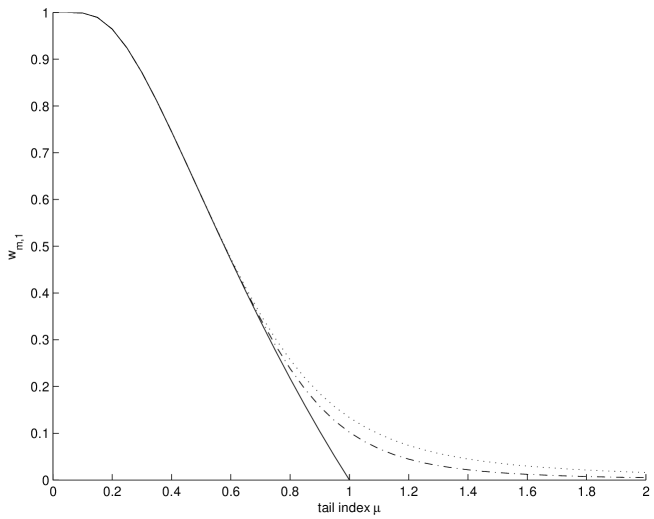
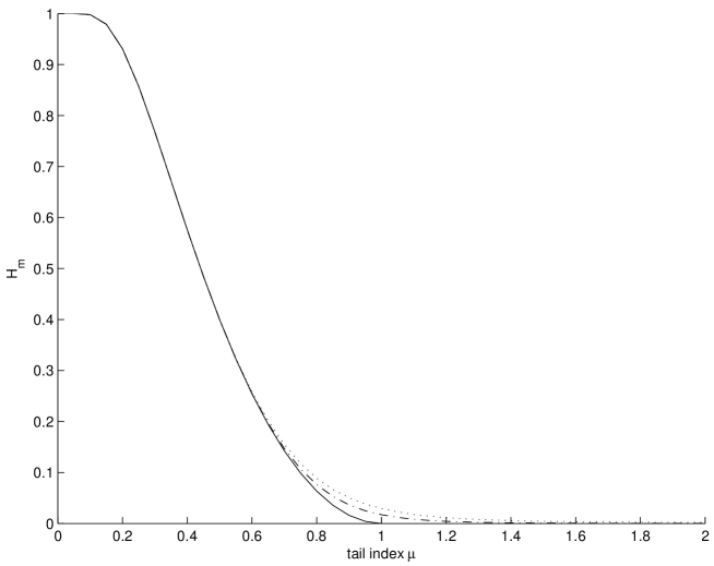
Figure 1: Concentration of the market portfolio. The upper panel shows the weight of the largest firms in the market portfolio as a function of the tail index $\mu$ of the Pareto distribution of firm sizes. The lower panel shows the Herfindahl index of the market portfolio as a function of the tail index $\mu$ of the Pareto distribution of firm sizes. In both cases, the continuous line provides the values in the limit of an infinite economy while the dotted and dash-dotted curves refers to the cases of an economy with one thousand and ten thousand firms respectively.

In order to illustrate this situation, the upper panel of figure 1 depicts the value of the weight of the largest firm in the market portfolio while the lower panel shows the Herfindahl index as a function of $\mu$. The plain curves show the limit situation of an infinite economy while the dotted and dash-dotted curves account for the effect of a finite economy: the dotted curve refers to the case where only one thousand companies are traded while the dash-dotted curve corresponds to an economy with ten thousand firms. Clearly, finite economy size effects cannot be neglected for market sizes as found in the real economy.

[Insert Figure 1 about here]

To be a little bit more general, we now consider the case where the firm sizes are randomly drawn from a power law distribution of size. By application of the generalized law of large numbers (?, ?, ?) and using standard results on the limit distribution of self-normalized sums (?, ?), we can state that

Proposition 1.

The asymptotic behavior of the concentration index $H_{N}$ is the following:

1. provided that ${\rm E}[S^{2}]<\infty$,

   $$H_{N}=\frac{1}{N}\frac{{\rm E}\left[S^{2}\right]}{{\rm E}\left[S\right]^{2}}+o_{p}(1/N),$$

2. provided that $S$ is regularly varying with tail index $\mu=2$ and $s^{\mu}\cdot\Pr\left[S>s\right]\rightarrow c$ as $s\rightarrow\infty$,

   $$H_{N}=\frac{c}{{\rm E}\left[S\right]^{2}}\frac{\ln N}{N}+o_{p}\left(\frac{1}{N\ln N}\right),$$

3. provided that $S$ is regularly varying with tail index $\mu\in(1,2)$ and $s^{\mu}\cdot\Pr\left[S>s\right]\rightarrow c$ as $s\rightarrow\infty$,

   $$H_{N}=\left[\frac{\pi c}{2\Gamma\left(\frac{\mu}{2}\right)\sin\frac{\mu\pi}{4}}\right]^{2/\mu}\frac{1}{{\rm E}\left[S\right]^{2}}\cdot\frac{1}{N^{2-2/\mu}}\cdot\xi_{N}+o_{p}\left(\frac{1}{N^{2-2/\mu}}\right)~{},$$

   where $\xi_{N}$ is a sequence of positive random variables with stable limit law $S(\mu/2,1)$,

4. provided that $S$ is regularly varying with tail index $\mu=1$ and $s^{\mu}\cdot\Pr\left[S>s\right]\rightarrow c$ as $s\rightarrow\infty$,

   $$H_{N}=\frac{\pi}{2\cdot{\ln^{2}N}}\cdot\xi_{N}+O_{p}\left(\frac{1}{\ln^{3}N}\right),$$

   where $\xi_{N}$ is a sequence of positive random variables with stable limit law $S(1/2,1)$,

5. provided that $S$ is regularly varying with tail index $\mu\in(0,1)$ and $s^{\mu}\cdot\Pr\left[S>s\right]\rightarrow c$ as $s\rightarrow\infty$,

   $$H_{N}=\frac{4}{\pi^{1/\mu}}\left[\Gamma\left(\frac{1+\mu}{2}\right)\cos\frac{\pi\mu}{4}\right]^{2/\mu}\cdot\frac{\xi_{N}}{\zeta_{N}^{2}},$$

   where $\xi_{N}$ and $\zeta_{N}$ are two sequences of strongly correlated positive random variables that converge in law to $S(\mu/2,1)$ and $S(\mu,1)$ respectively,

6. provided that $S$ is slowly varying,

   $$H_{N}\rightarrow 1,\quad\text{a.s.}$$

As a consequence of the fourth statement of the proposition above, for economies in which the distribution of firm sizes follows Zipf’s law ($\mu=1$) the asymptotic behavior of the concentration index $H_{N}$ of the market portfolio is given by

$$H_{N}\simeq\frac{\pi}{2\cdot\left(\ln N\right)^{2}}\cdot\xi_{N},$$ (9)

where $\xi_{N}$ is a sequence of positive random variables with stable limit law $S(1/2,1)$, namely the Lévy law with density

$$f(x)=\frac{1}{\sqrt{2\pi}}\cdot x^{-3/2}{\rm e}^{-\frac{1}{2x}},\quad x\geq 0.$$ (10)

This shows that, even if the concentration of the market portfolio goes to zero in the limit of an infinite economy, it goes to zero extremely slowly as the size $N$ of the economy diverges. Accounting for the fact that the median value of the Lévy law (10) is approximately equal to $2.198$, a typical value of $H_{N}$ is $4-5\%$ for a market where $7000$ to $8000$ assets are traded, which is much higher than the concentration index of a well-diversified portfolio – typically the equally-weighted portfolio – which should be of the order of $0.012-0.014\%$. Intuitively, $H_{N}\simeq 4-5\%$ means that there are only about $1/H_{n}\simeq 20-25$ effective assets in a typical portfolio supposedly well-diversified on $7000-8000$ assets.

This simple illustrative example shows, roughly speaking, that the market portfolio reflects the behavior of the 20 to 25 largest assets traded on the market. In this context, one can wonder (i) how the market portfolio alone could explain the expected return on any asset, irrespective of its size, as predicted by the CAPM and (ii) if it is actually optimal for a rational investor to put her money in this risky portfolio alone, as proposed by the two-fund separation theorem. This suggests that the lack of diversification of the market portfolio is responsible, to a large extent, for the failure of the CAPM to explain the cross-section of stock returns. This failure has been documented in particular by Fama and French (?, ?), who find basically no support for the CAPM’s central result of a positive relation between expected returns and the global market risk (quantified by the beta parameter). This therefore raises the question of the existence of a concentration premium.

Many authors have proposed alternative or additional factors in the quest to cure the deficiencies of the CAPM and provide explanations for the so-called pricing anomalies. Three main classes of additional factors can be distinguished: macro-economic factors, firm-specific factors and behavioral factors.

• Macro-economic factors. The positive or negative impact on stock prices of macro-economic factors such as interest rates (?), exchange rates (?, ?), real output (?, ?), inflation and money supply (?, ?, ?, ?, 1985), aggregate consumption (?, and references therein), oil prices (?, ?, ?), labor income (?, ?) and so on, has been underlined in many studies based on the APT (?, ?, ?) or in the context of equilibrium (?, ?).

• Firm-specific factors. The fact that industry sector groupings may be important in the study of the return generating process has been stressed for a long time (?, ?). Similarly, the importance of market capitalization (or small-firm effect) has been documented in the early eighties by ? and ? while ? and ? underlined the role of the book-to-market ratio. If other ratios such as the earnings-to-price ratio (?) and the dividend yield (?, ?, ?) for instance, also predict future returns, most of the attention has been drawn to the size and the book-to-market effect during the past decade as a result of their superior performance to explain the cross-section of stock returns (?, 1993,1995,1996). Among various interpretation of the explaining power of the size and the book-to-market ratio, ? and ? have considered breaking the beta of a stock with the market portfolio into two components, one reflecting news about the market’s future cash flows and one reflecting news about the market’s discount rates in order explain the size and value “anomalies” in stock returns.

• Behavioral factors. Two major issues have been considered. On the one hand, ? and ? have proposed to account for the departure of the distributions of returns from normality and for the sensibility of the investors for the skewness and kurtosis of the distribution of stock returns. The relevance of this approach has been underlined by ? and ? who have tested the role of the asymmetry in the risk premium by accounting for the skewness of the distribution of returns. Along the same line, many other extensions have been presented such as the VaR-CAPM (?), in order to account more carefully for the risk perception of investors. On the other hand, several studies have developed phenomenological models capturing the reversal of long-term returns (?, ?, ?, 1987) and the continuation of short-term trends (?, ?, ?, ?).

Most of these factors actually provide a significant improvement in explaining the cross-section of asset returns. However they do not provide a clear identification of the most prominent ones. Even if the Fama and French three factor model is now widely recognized as the benchmark, the reasons for its superiority in explaining the cross-section of asset returns are still debated. It is in this context that we propose to focus on the consequences of the undisputable fact that the market portfolio is highly concentrated on a small number of very large companies and therefore can obviously not account for the behavior of the smallest ones. As we are going to demonstrate, this will allow us to rationalize the size effect, in relation with what we propose to call a “diversification factor,” which, to some extent, also justify the relevance of the book-to-market factor.

2 Internal consistency conditions of factor models and their consequences on diversification

Under the assumption that the return on the market portfolio is a factor explaining the return on individual assets, our demonstration is based on two ingredients.

• The internal consistency condition states that the market portfolio is made of the assets whose returns it is supposed to explain. As a consequence, there are correlations between the disturbance terms.

• The lack of diversification of the market portfolio (associated with the fat tail distribution of firm sizes) make these correlations non-negligible, giving birth to an additional factor which significantly contributes to the asymptotic variance of a priori well-diversified portfolios.

2.1 The factor model

Consider an economy with $N$ firms whose returns on stock prices are determined according to the following equation

$$\vec{r}=\vec{\alpha}+\vec{\beta}_{m}\cdot\left[r_{m}-{\rm E}\left[r_{m}\right]\right]+B\vec{\phi}+\vec{\varepsilon},$$ (11)

where

• $\vec{r}$ is the random $N\times 1$ vector of asset returns;

• $\vec{\alpha}={\rm E}\left[\vec{r}\right]$ is the $N\times 1$ vector of asset return mean values. We do not make any assumption neither on the ex-ante mean-variance efficiency of the market portfolio, nor on the absence of arbitrage opportunity, so that $\vec{\alpha}$ is not, a priori, specified;

• $r_{m}$ is the random return on the market portfolio;

• $\vec{\beta}_{m}$ is the $N\times 1$ vector of the factor loadings of the market factor;

• $\vec{\phi}$ is the random $N\times 1$ vector of risk factors $\phi_{i}$ which are assumed to have zero mean (${\rm E}\left[\phi_{i}\right]=0$), unit variance, are uncorrelated with each other and with $r_{m}$;

• $B$ is the $N\times q$ matrix of factor loadings;

• $\vec{\varepsilon}$ is the random $N\times 1$ vector of disturbance terms with zero average ${\rm E}\left[\vec{\varepsilon}\right]=\vec{0}$ and covariance matrix $\Omega={\rm E}\left[\vec{\varepsilon}\cdot\vec{\varepsilon}\right]$. The disturbance terms are assumed to be uncorrelated with the market return $r_{m}$ and the factors $\phi_{i}$.

It would be natural to assume that (i) $\Omega$ is diagonal in order to have the $i^{th}$ contribution of $\vec{\varepsilon}$ embodying the specific risk contribution to the $i^{th}$ asset but, as we shall see in the sequel, the internal consistency condition makes this impossible and forces the disturbances $\vec{\varepsilon}$ to be correlated. A weaker hypothesis on $\Omega$ would be that (ii) all its eigenvalues are uniformly bounded from above by some constant $\lambda$ (i.e., the bound is independent of the size of the economy: $\displaystyle\forall N,\max_{||x||=1}x^{\prime}\Omega x\leq\lambda$). This implies that the covariance matrix of the stock returns defined as

$$\Sigma={\rm E}\left[\left(\vec{r}-\vec{\alpha}\right)\left(\vec{r}-\vec{\alpha}\right)^{\prime}\right]=\vec{\beta}\vec{\beta}^{\prime}\cdot{\rm Var}~{}r_{m}+BB^{\prime}+\Omega,$$ (12)

where the prime denotes the transpose operator, has an approximate $q+1$ factor structure, according to the definition in ? and ?. But these two assumptions (i) and (ii) are in fact equivalent, as shown by ?. Indeed, a simple repackaging of the $N$ security returns into $N$ new returns constructed by forming $N$ portfolios of the primitive assets allows one to get a new formulation of expression (11) with mutually uncorrelated disturbance terms.

To understand why the disturbance terms cannot be uncorrelated, let us first denote by $\vec{w}_{m}$ the vector of the weights of the market portfolio. Accounting for the fact that the market factor is itself built upon the universe of assets that it is supposed to explain, the model must necessarily fulfill the internal consistency relation

$$r_{m}=\vec{w}_{m}^{\prime}\cdot\vec{r}.$$ (13)

Left-multiplying (11) by $\vec{w}_{m}^{\prime}$, the internal consistency condition (13) implies the following relationship

$$\left[{\vec{w}^{\prime}}_{m}\cdot{\vec{\beta}}-1\right]\cdot\left(r_{m}-{\rm E}\left[r_{m}\right]\right)+w_{m}^{\prime}B\vec{\phi}+{\vec{w}^{\prime}}_{m}\cdot{\vec{\varepsilon}}=0~{}.$$ (14)

Then, by our assumption of absence of correlation between $r_{m}$, $\vec{\phi}$ and $\vec{\varepsilon}$, it follows trivially that

$$\vec{w}_{m}^{\prime}\cdot\vec{\varepsilon}=0\qquad\text{almost surely},$$ (15)

while

$$\vec{w}_{m}^{\prime}\cdot\vec{\beta}=1\quad\text{and}\qquad\vec{w}_{m}^{\prime}B=0~{}.$$ (16)

Several authors have pointed out a consequence of the internal consistency condition that the market portfolio is made of (or can be replicated by) the assets they are intended to explain (?, ?). An a priori important consequence of this internal consistency condition is the breakdown of the standard assumption of independence (or, at least, of the absence of correlation) between the non-systematic components of the returns of securities. In other words, the standard factor model decompositions assume that the disturbance terms for security $i$ are uncorrelated with the comparable components for security $j$. But, this cannot be strictly the case as can be seen from the above derivation. This presence of correlations between the disturbance terms may a priori pose problems in the pricing of portfolio risks: only when the disturbance terms can be averaged out by diversification can one conclude that the only non-diversifiable risk of a portfolio is born out by the contribution of the market portfolio which is weighted by the beta of the portfolio under consideration. Previous authors have suggested that this is indeed what happens in economies in the limit of a large market $N\to\infty$, for which the correlations between the disturbance terms vanish asymptotically and the internal consistency condition seems irrelevant. For example, while ? concluded that, as a consequence of equation (15), at least two of the disturbances, say $\varepsilon_{i}$ and $\varepsilon_{j}$, must be negatively correlated, he suggested that this problem may disappear in economies with infinitely many securities. Actually, we show below that this apparently quite reasonable line of reasoning does not tell the whole story: even for economies with infinitely many securities, when the companies exhibit a large distribution of sizes as they do in reality, the constraint (15) can lead to the important consequence that the risk born out by an investor holding a well-diversified portfolio does not reduce to the market risk in the limit of a very large portfolio, as usually believed. A significant proportion of “specific risk” may remain which cannot be diversified away by a simple aggregation of a very large number of assets.

2.2 Correlation structure of the disturbance terms

The fact that the disturbance terms $\vec{\varepsilon}$ in the market model (11) are correlated according to the condition (15) means that there exists at least one common “factor” $f$ to the $\varepsilon$’s, so that $\vec{\varepsilon}$ can be expressed as

$$\vec{\varepsilon}=\vec{\gamma}\cdot f+\vec{\eta}~{},$$ (17)

where $\vec{\gamma}$ is the vector of loading of the factor $f$. The factor $f$ could be chosen a priori such as to explain one of the many anomalies reported in the previous section. But, as recalled, we want to move away from this logic of invoking macro-economic, firm-specific or behavioral factors. We prefer to focus on the parsimonious single market factor model, and just account for the lack of diversification of the market portfolio which calls for a diversification premium. As a bonus, we will see that this strategy turns out to provide a fundamental basis of explaining a significant part of the pricing anomalies. Our only requirement is that the covariance matrix of $\vec{\varepsilon}$ exhibits an eigenvalue that goes to infinity in the limit of an infinite economy, when $H_{N}$ does not go to zero. In contrast, when $H_{N}$ goes to zero as $N\to\infty$, the largest eigenvalue should remain bounded. This requirement derives simply from the results of ? and ?, who have linked the existence of $K$ unbounded eigenvalues (in the limit $N\to\infty$) of the covariance matrix of the asset returns to a unique approximate factor structure, such that the $K$ associated eigenvectors converge and play the role of $K$ factor loadings.

For simplicity, we choose $\vec{\eta}$ to be a vector of uncorrelated residuals with zero mean. Since $\vec{w}_{m}^{\prime}\vec{\varepsilon}=0$, $f$ and $\vec{\eta}$ are not independent from one another. More precisely, we have

$$f=-\frac{\vec{w}_{m}^{\prime}\vec{\eta}}{\vec{w}_{m}^{\prime}\vec{\gamma}},$$ (18)

provided that $\vec{w}_{m}^{\prime}\vec{\gamma}\neq 0$; if not, the random vector $\vec{\eta}$ would have to satisfy $\vec{w}_{m}^{\prime}\vec{\eta}=0$, which contradicts our assumption of an absence of correlations between the components of $\vec{\eta}$. Therefore, in this framework, $f$ is not actually a factor – it should be uncorrelated with $\vec{\eta}$ if it was – but is rather an “endogenous” factor. The market model (11) then becomes

$$\vec{r}=\vec{\alpha}+\vec{\beta}\cdot\left[r_{m}-{\rm E}\left[r_{m}\right]\right]+\vec{\gamma}\cdot f+\vec{\eta},$$ (19)

with

• ${\rm Cov}~{}(r_{m},f)={\rm Cov}~{}(r_{m},\vec{\eta})=0$, as the result of the absence of correlation between $r_{m}$ and $\vec{\varepsilon}$,

• ${\rm Var}~{}\vec{\eta}=\Delta$, where $\Delta$ is a diagonal matrix,

• ${\rm Var}~{}f=\frac{\vec{w}_{m}^{\prime}\Delta\vec{w}_{m}}{\left(\vec{w}_{m}^{\prime}\vec{\gamma}\right)^{2}}$, and

• ${\rm Cov}~{}(f,\vec{\eta})=-\frac{1}{\vec{w}_{m}^{\prime}\vec{\gamma}}\cdot\vec{w}_{m}^{\prime}\Delta$.

In order to understand and illustrate the relevance and the limits of the assertion according to which the existence of correlations between two disturbance terms $\varepsilon_{i}$ and $\varepsilon_{j}$ should be negligible in an infinite size market (?, ?), let us now evaluate their typical magnitude. To simplify the notations, let us rescale without loss of generality the vector $\vec{\gamma}$ by $\vec{w}_{m}^{\prime}\vec{\gamma}$, so that the relation (18) becomes

$$f=-\vec{w}_{m}^{\prime}\vec{\eta},$$ (20)

with $\vec{w}_{m}^{\prime}\vec{\gamma}=1$. The covariance matrix $\Omega$ of $\vec{\varepsilon}$ is

$$\Omega=\left(\vec{w}_{m}^{\prime}\Delta\vec{w}_{m}\right)\vec{\gamma}\vec{\gamma}^{\prime}-\vec{\gamma}\vec{w}_{m}^{\prime}\Delta-\Delta\vec{w}_{m}\vec{\gamma}^{\prime}+\Delta,$$ (21)

and the correlation between $\varepsilon_{i}$ and $\varepsilon_{j}$ ($i\neq j$) is

$$\rho_{ij}=\frac{\left(\vec{w}_{m}^{\prime}\Delta\vec{w}_{m}\right)\gamma_{i}\gamma_{j}-\gamma_{i}w_{m,j}\Delta_{jj}-\gamma_{j}w_{m,i}\Delta_{ii}}{\sqrt{\left[\left(\vec{w}_{m}^{\prime}\Delta\vec{w}_{m}\right)\gamma_{i}^{2}-2\gamma_{i}w_{m,i}\Delta_{ii}+\Delta_{ii}\right]\cdot\left[\left(\vec{w}_{m}^{\prime}\Delta\vec{w}_{m}\right)\gamma_{j}^{2}-2\gamma_{j}w_{m,j}\Delta_{jj}+\Delta_{jj}\right]}}~{}.$$ (22)

For illustration purpose, let us assume that all the $\gamma_{i}$’s are equal to one (the condition $\vec{w}_{m}^{\prime}\vec{\gamma}=1$ is then automatically satisfied from the normalization of the weights $\vec{w}_{m}$) and that $\Delta_{ii}=\Delta$ for all $i$’s. The cumbersome relation (22) simplifies into

$$\rho_{ij} = \displaystyle\frac{H_{N}-w_{m,i}-w_{m,j}}{\sqrt{\left(1+H_{N}-2w_{m,i}\right)\left(1+H_{N}-2w_{m,j}\right)}},$$ (23)

$$= \displaystyle\frac{H_{N}}{1+H_{N}}\cdot\left(1+O(w_{m,i(j)}/H_{N})\right)~{}.$$ (24)

Then, expression (24) shows that, provided that the market portfolio is sufficiently well-diversified, namely provided that the weight of each asset and the concentration index goes to zero in the limit of a large market ($N\to\infty$), the correlations $\rho_{ij}$ between any two disturbance terms goes to zero as usually assumed. However, the largest eigenvalue of the correlation matrix, associated with the (asymptotic) eigenvector $\vec{1}=\left(1,1,\dots,1\right)^{\prime}$, is $\lambda_{\max,N}\simeq N\cdot\frac{H_{N}}{1+H_{N}}$ and goes to infinity, as the size of the economy growths unbounded, as soon as $H_{N}$ goes to zero more slowly than $1/N$. This clearly shows that the correlations between the disturbance terms are not necessarily negligible.

The question, that we now have to address, is whether these weak correlations may challenge the usual assumption that well-diversified portfolios do not bear additional non-diversified sources of risks. For this, let us consider a well diversified portfolio $\vec{w}_{p}$, i.e., a portfolio such that $||w_{p}||^{2}\rightarrow 0$ as the size of the economy goes to infinity. From equation (21), the residual variance of this portfolio, namely the part of the variance of the portfolio that cannot be ascribed to systematic risk factors, reads

$$w_{p}^{\prime}\Omega w_{p}=\left(\vec{w}_{m}^{\prime}\Delta\vec{w}_{m}\right)\left(\vec{\gamma}\vec{w}_{p}^{\prime}\right)^{2}-2\left(\vec{w}_{m}^{\prime}\Delta\vec{w}_{p}\right)\left(\vec{\gamma}^{\prime}\vec{w}_{p}\right)+\vec{w}_{p}^{\prime}\Delta\vec{w}_{p}^{\prime}~{}.$$ (25)

In addition to our previous hypothesis that $\Delta$ is a diagonal matrix, we assume that its entries are uniformly bounded from below by some positive constant $c_{1}$ and from above by some constant $c_{2}<\infty$ and that $|\vec{\gamma}\vec{w}_{p}^{\prime}|$ is uniformly bounded from below by some positive constant $c^{\prime}$ and from above by some finite constant $c^{\prime\prime}$ (this is the case, for instance, when one considers $\vec{\gamma}=\vec{1}$, which is compatible with the requirement $w_{m}^{\prime}\cdot\vec{\gamma}=1$ assumed in the representation (21)). Then

$$\vec{w}_{p}^{\prime}\Delta\vec{w}_{p}^{\prime} \leq c_{2}\cdot||\vec{w}_{p}||^{2}\rightarrow 0,$$ (26)

$$\left|\left(\vec{w}_{m}^{\prime}\Delta\vec{w}_{p}\right)\left(\vec{\gamma}^{\prime}\vec{w}_{p}\right)\right| \leq c_{2}\cdot c^{\prime\prime}\cdot||w_{m}||\cdot||w_{p}||\rightarrow 0,$$ (27)

and

$$c_{1}\cdot c^{\prime}\cdot||w_{m}||^{2}\leq\left(\vec{w}_{m}^{\prime}\Delta\vec{w}_{m}\right)\left(\vec{\gamma}\vec{w}_{p}^{\prime}\right)^{2}\leq c_{2}\cdot c^{\prime\prime}\cdot||w_{m}||^{2},$$ (28)

so that

$$w_{p}^{\prime}\Omega w_{p}\sim K\cdot H_{N},\quad K>0,~{}~{}\text{as}~{}~{}~{}N\rightarrow\infty.$$ (29)

Therefore, the residual variance $\vec{w}_{p}^{\prime}\Omega\vec{w}_{p}$ of any “well-diversified portfolio” $\vec{w}_{p}$ goes to zero, as the size $N$ of the economy goes to infinity, if and only if the concentration index $H_{N}$ of the market portfolio goes to zero. In the case of a real economy, section 1 has shown that the Herfindahl index $H_{N}$ of the market portfolio goes to zero but at the particularly slow decay rate of $1/(\ln N)^{2}$. As a consequence, the residual variance may still account for a significant part of the total portfolio variance. We will give a numerical example in the next paragraph providing a more precise statement concerning the behavior of the residual variance of the equally-weighted portfolio.

2.3 Asymptotic behavior of the variance of the excess return of the equally-weighted portfolio

In order to investigate more precisely the impact of the correlations between the disturbance terms induced by the condition of internal consistency on the variance of the returns of a “well-diversified” portfolio, we consider first the simple case of the equally-weighted portfolio whose composition is given by the vector $\vec{w}_{e}=\frac{1}{N}\vec{1}$. Algebraic manipulations yield

$${\rm Var}~{}r_{e}={\beta_{e}}^{2}\cdot{\rm Var}~{}r_{m}+{\bar{\gamma}_{N}}^{2}\cdot\frac{\sum_{i=1}^{N}S_{i}^{2}\Delta_{ii}}{\left(\sum_{i=1}^{N}S_{i}\gamma_{i}\right)^{2}}-2\bar{\gamma}_{N}\frac{1}{N}\cdot\frac{\sum_{i=1}^{N}S_{i}\Delta_{ii}}{\sum_{i=1}^{N}S_{i}\gamma_{i}}+\frac{1}{N}\left(\frac{1}{N}\sum_{i=1}^{N}\Delta_{ii}\right),$$ (30)

where $r_{e}$ denotes the return on the equally-weighted portfolio and $\beta_{e}$ its beta with the market factor. We have reintroduced the explicit dependence on the term $\sum_{i=1}^{N}w_{m,i}\gamma_{i}$ (no more assumed to be scaled to the value $1$) and have explicited the fact that the market weight of firm $i$ is $w_{m,i}=S_{i}/\sum_{i=1}^{n}S_{i}$.

Two of the four terms in the right-hand-side (r.h.s.) of expression (30) are standard. The first term ${\beta_{e}}^{2}\cdot{\rm Var}~{}r_{m}$ is the traditional contribution of the market risk factor weighted by the beta of the portfolio. The last rightmost term in the r.h.s. of (30) represents the usual contribution of the diversifiable risk of the portfolio when one assumes that the disturbance terms are uncorrelated and therefore represents the specific sources of risk. The two other terms are new and result from the existence of correlations between the disturbances. In the absence of such correlations, ${\bar{\gamma}}$ would be zero and these two terms disappear.

Assuming that the $\Delta_{ii}$’s are $N$ iid (positive) random variables with finite expected value ${\rm E}\left[\Delta_{ii}\right]<\infty$, we get that $\frac{1}{N^{2}}\sum_{i=1}^{N}\Delta_{ii}$ and $\frac{1}{N}\left(\bar{\gamma}_{N}\cdot\frac{\sum_{i=1}^{N}S_{i}\Delta_{ii}}{\sum_{i=1}^{N}S_{i}\gamma_{i}}\right)$ are $O_{p}\left(1/N\right)$, irrespective of the fact that the distribution of firm sizes admits or does not admit a finite mean. This implies that, in the limit of large $N$, the third and fourth terms in the r.h.s. of expression (30) can be neglected, leading to

$${\rm Var}~{}r_{e}={\beta_{e}}^{2}\cdot{\rm Var}~{}r_{m}+{\bar{\gamma}_{N}}^{2}\cdot\frac{\sum_{i=1}^{N}S_{i}^{2}\Delta_{ii}}{\left(\sum_{i=1}^{N}S_{i}\gamma_{i}\right)^{2}}+O_{p}(1/N).$$ (31)

The fact that the fourth term in expression (30) disappears in the limit $N\to\infty$ is not surprising since it recovers the standard result on the diversification of the idiosyncratic risks. More interestingly, the fact that the third term in (30) also goes to zero as $1/N$ means that it does not introduce (in the limit of a large market) an additional risk worth considering.

Proposition 2 below reveals through expression (31) that the only significant additional contribution to the risks of the equally-weighted portfolio stems from the term

$${\bar{\gamma}_{N}}^{2}\cdot\frac{\sum_{i=1}^{N}S_{i}^{2}\Delta_{ii}}{\left(\sum_{i=1}^{N}S_{i}\gamma_{i}\right)^{2}}~{},$$ (32)

which is nothing but the variance (conditional of the $\gamma_{i}$’s and the $S_{i}$’s) of the term $\bar{\gamma}_{N}\cdot f$ resulting from the expression of the market model (19).

By the same kind of arguments as in Proposition 1, we get that the contribution (32) exhibits three different behaviors. Either the variance of the distribution of firm sizes is finite and the term (32) goes to zero has $1/N$, or only the mean of the distribution of firm sizes exists and the term (32) goes to zero at a much slower rate or, finally, if the mean of the distribution of firm sizes does not exist, the additional risk term (32) converges to some finite positive value. More precisely, we can state the following results:

Proposition 2.

Assuming that the $\gamma_{i}$’s are iid random variables such that ${\rm E}\left[|\gamma|\right]<\infty$, and that the $\Delta_{ii}$’s are iid positive random variables such that ${\rm E}[\Delta_{ii}]=\bar{\Delta}<\infty$, the asymptotic behavior of the variance of the equally-weighted portfolio is the following:

1. provided that ${\rm E}[S^{2}]<\infty$,

   $${\rm Var}~{}r_{e}={\beta_{e}}^{2}\cdot{\rm Var}~{}r_{m}+O_{p}(1/N),$$

2. provided that $S$ is regularly varying with tail index $\mu=2$ and $s^{\mu}\cdot\Pr\left[S>s\right]\rightarrow c>0$, as $s$ goes to infinity,

   $${\rm Var}~{}r_{e}={\beta_{e}}^{2}\cdot{\rm Var}~{}r_{m}+\frac{c\cdot\bar{\Delta}}{{\rm E}\left[S\right]^{2}}\frac{\ln N}{N}+o_{p}(\ln N/N),$$

3. provided that $S$ is regularly varying with tail index $\mu\in(1,2)$ and $s^{\mu}\cdot\Pr\left[S>s\right]\rightarrow c>0$, as $s$ goes to infinity,

   $${\rm Var}~{}r_{e}={\beta_{e}}^{2}\cdot{\rm Var}~{}r_{m}+\left[\frac{\pi c{\rm E}\left[\Delta^{\mu/2}\right]}{2\Gamma\left(\frac{\mu}{2}\right)\sin\frac{\mu\pi}{4}}\right]^{2/\mu}\frac{1}{{\rm E}\left[S\right]^{2}}\cdot\frac{1}{N^{2-2/\mu}}\cdot\xi_{N}+o_{p}\left(\frac{1}{N^{2-2/\mu}}\right)~{},$$

   where $\xi_{N}$ is a sequence of positive random variables with stable limit law $S(\mu/2,1)$,

4. provided that $S$ is regularly varying with tail index $\mu=1$ and $s^{\mu}\cdot\Pr\left[S>s\right]\rightarrow c>0$, as $s$ goes to infinity,

   $${\rm Var}~{}r_{e}={\beta_{e}}^{2}\cdot{\rm Var}~{}r_{m}+\frac{\pi~{}{\rm E}\left[\Delta^{1/2}\right]^{2}}{2}\frac{{\rm E}\left[\gamma\right]^{2}}{{\rm E}\left[|\gamma|\right]^{2}}\frac{1}{\ln^{2}N}\cdot\xi_{N}+o_{p}\left(1/\ln^{2}N\right),$$

   where $\xi_{N}$ is a sequence of positive random variables with stable limit law $S(1/2,1)$,

5. provided that $S$ is regularly varying with tail index $\mu\in(0,1)$ and $s^{\mu}\cdot\Pr\left[S>s\right]\rightarrow c>0$, as $s$ goes to infinity,

   $${\rm Var}~{}r_{e}={\beta_{e}}^{2}\cdot{\rm Var}~{}r_{m}+{\rm E}\left[\Delta^{\mu/2}\right]^{2/\mu}\frac{{\rm E}\left[\gamma\right]^{2}}{{\rm E}\left[|\gamma|^{\mu}\right]^{2/\mu}}\frac{4}{\pi^{1/\mu}}\left[\Gamma\left(\frac{1+\mu}{2}\right)\cos\frac{\pi\mu}{4}\right]^{2/\mu}\cdot\frac{\xi_{N}}{\zeta_{N}^{2}}+o_{p}(1),$$

   where $\xi_{N}$ and $\zeta_{N}$ are two sequences of strongly correlated positive random variables that converge in law to $S(\mu/2,1)$ and $S(\mu,\beta_{\gamma})$ with $\beta_{\gamma}=\frac{{\rm E}\left[\gamma^{\mu}\cdot 1_{\gamma>0}\right]-{\rm E}\left[|\gamma|^{\mu}\cdot 1_{\gamma<0}\right]}{{\rm E}\left[|\gamma|^{\mu}\right]}$ respectively.

Focusing on the case where $\mu$ is equal (or close) to one, as in real markets, proposition 2 tells us that the asymptotic behavior of the variance of the equally weighted portfolio is given by

$${\rm Var}~{}r_{e}={\beta_{e}}^{2}\cdot{\rm Var}~{}r_{m}+\frac{\pi\cdot{\rm E}\left[\gamma\right]^{2}\cdot{\rm E}\left[\Delta^{1/2}\right]^{2}}{2\cdot{\rm E}\left[|\gamma|\right]^{2}\cdot\left(\ln N\right)^{2}}\cdot\xi_{N}+o_{p}\left(1/\left(\ln N\right)^{2}\right),$$ (33)

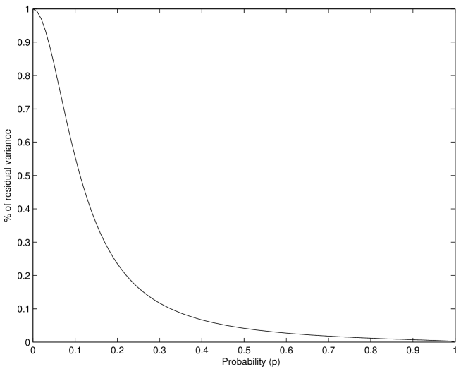
Figure 2: Contribution of the residual variance to the total variance. The figure shows the probability $p$ to reach or exceed a given contribution level, in percentage, of the residual variance to the total variance of the return on the equally weighted portfolio in a market with 7000-8000 traded assets and with a distribution of firm sizes given by Zipf’s law ($\mu=1$).

where $\xi_{N}$ is a sequence of positive random variables with stable limit law $S(1/2,1)$ whose density is given by (10). Expression (33) implies that the variance of the equally-weighted portfolio, while asymptotically proportional to the variance of the market portfolio, receives a significant contribution due to the internal consistent condition together with the Zipf distribution of company sizes. This additional contribution decays to zero extremely slowly with the number $N$ of companies in the economy. For instance, (i) assuming that the variance $\Delta_{ii}$ of the residuals $\eta_{i}$ is the same for all of them and, a priori, of the same order as the variance of the market return: $\Delta_{ii}\sim{\rm Var}~{}r_{m}$, (ii) considering that the ratio $\frac{{\rm E}\left[\gamma\right]^{2}}{{\rm E}\left[|\gamma|\right]^{2}}$ is of the order of one and (iii) accounting for the fact that the median value of the Lévy law is approximately equal to $2.198$, the additional term is typically of the order of $\frac{\pi}{\left(\ln N\right)^{2}}\cdot{\rm Var}~{}r_{m}$. So, assuming that $\beta_{e}$ is about one and considering a market where $7000$ to $8000$ assets are traded, the typical amplitude of the additional term represents $5\%$ of the total variance of the equally-weighted portfolio. More precisely, in one case out of two, the contribution of the additional term is larger than $5\%$ of the total variance. Figure 2 presents the probability to reach or exceed a given level for the contribution of the residual variance to the total variance, in an economy with 7000-8000 traded assets. In one case out at four ($p=0.25$), the contribution of the residual variance to the total variance is larger than $15\%$; in one case out ten ($p=0.1$), it represents more than $50\%$.

[ Insert Figure 2 about here]

2.4 Relation with the concentration of the market portfolio

The variance of the term $\bar{\gamma}_{N}\cdot f$ given by (32) cannot be easily related to observable market variables since it is a mixture of the firm sizes (which are observable) and of the not directly accessible underlying variables $\gamma_{i}$’s and $\Delta_{ii}$’s which describe the correlation structure of the disturbances $\vec{\varepsilon}$ in the model (11). Nevertheless, as a consequence of the assumption that the $\gamma_{i}$’s and $\Delta_{ii}$’s have finite expectations, the behavior of the term $\frac{\sum_{i=1}^{N}S_{i}^{2}\Delta_{ii}}{\left(\sum_{i=1}^{N}S_{i}\gamma_{i}\right)^{2}}$ is the same as that of $\frac{\sum_{i=1}^{N}S_{i}^{2}}{\left(\sum_{i=1}^{N}S_{i}\right)^{2}}$ which is nothing but the Herfindahl index $H_{N}$ of the market portfolio since

$$H_{N}\equiv\sum_{i=1}^{N}w_{m,i}^{2}=\frac{\sum_{i=1}^{N}S_{i}^{2}}{\left(\sum_{i=1}^{N}S_{i}\right)^{2}}~{}.$$ (34)

In fact, propositions 1 and 2 are closely related. Loosely speaking, these two propositions can be summarized as follows

$${\rm Var}~{}r_{e}\stackrel{{\scriptstyle law}}{{\simeq}}\beta_{e}^{2}\cdot{\rm Var}~{}r_{m}+K_{\mu}\cdot H_{N},$$ (35)

where

$$K_{\mu}=\left\{\begin{array}[]{lr}\displaystyle{\rm E}\left[\Delta\right],&\mu\geq 2,\\ \displaystyle{\rm E}\left[\Delta^{\mu/2}\right]^{2/\mu},&1<\mu<2,\\ \displaystyle{\rm E}\left[\Delta^{\mu/2}\right]^{2/\mu}\cdot\frac{{\rm E}\left[\gamma\right]^{2}}{{\rm E}\left[|\gamma|^{\mu}\right]^{2/\mu}},&\mu\leq 1.\\ \end{array}\right.$$ (36)

Expression (35) has a simple intuitive meaning based upon the standard interpretation of the Herfindahl index as the inverse of the effective number of assets of a portfolio, if this portfolio was well-diversified (in fact, equally-weighted). Indeed, considering an equally-weighted portfolio made of $n$ assets, its Herfindahl index is $H=1/n$. Conversely, given a portfolio whose Herfindahl index is $H$, its effective number of assets, defined as the number of assets of an equally-weighted portfolio with the same value $H$ of the Herfindahl index, is $n_{eff}=1/H$. Therefore, considering that the real market is not made of $N$ $(\simeq 7000-8000)$ assets but actually of $N_{eff}=1/H_{N}$ $(\simeq 20-25)$ effective assets, equation (35) expresses the variance of the equally-weighted portfolio as the sum of two terms: the first one gives the variance of the portfolio resulting from the exposition to the market risk $\beta_{e}^{2}\cdot{\rm Var}~{}r_{m}$ while the second one represents the residual variance of the $N_{eff}=1/H_{N}$ assets. The constant $K_{\mu}$ appears as the average residual variance of the $N_{eff}$ assets. Thus, when the market portfolio is well-diversified, $H_{N}$ goes to zero, or equivalently, the number of effective assets goes to infinity so that, by virtue of the law of large numbers, the residual variance $K_{\mu}/N_{eff}$ goes to zero. In contrast, when the market portfolio is concentrated on a few assets, $H_{N}$ does not go to zero, the number of effective assets remains finite in the limit of an infinite economy and the residual variance does not go to zero.

For illustration purpose, we discuss in turn three cases. First, both propositions 1 and 2 show that the concentration index $H_{N}$ and the variance of $f$ are of the order of $1/N$, like the last two terms in the r.h.s. of expression (30), provided that the variance of the distribution of firm sizes is finite. As a consequence, for such distributions of firm sizes, the market portfolio is well diversified insofar as the concentration index is of the same order as the inverse of the number of assets in the portfolio. As a consequence, there is no additional non-diversifiable risk and, in the limit of a large market, we have

$${\rm Var}~{}r_{e}=\beta_{e}^{2}\cdot{\rm Var}~{}r_{m}+O_{p}(N^{-1}).$$ (37)

Let us consider the example of a distribution of firm sizes given by a Gamma law $\Gamma(r,\lambda)$. In such a case, it is well-known that the joint distribution of $\{w_{m,i}\}_{i=1}^{N-1}$ is a multivariate Beta law with parameter $r$ (?), which yields

$${\rm E}[H_{N}]=\frac{r+1}{r\cdot N+1},$$ (38)

in accordance with the fact that $H_{n}=\frac{1}{N}+o_{p}(1/N)$.

Second, if the distribution of firm sizes admits only a finite mean value and, in addition, is regularly varying at infinity with a tail index $\mu\in(1,2)$, the propositions 1 and 2 state that both the concentration index and the variance of $f$ are of the order of $1/N^{2\left(1-1/\mu\right)}$. As a consequence, the contribution to the total risk due to the second term in the r.h.s. of (30) decays to zero much slower than the decay $\sim 1/N$ of the two last terms. Then

$${\rm Var}~{}r_{e}=\beta_{e}^{2}\cdot{\rm Var}~{}r_{m}+\frac{C}{N^{2\left(1-\frac{1}{\mu}\right)}}+O_{p}(N^{-1}),\qquad\text{for some }C>0.$$ (39)

As an example, if the tail index of the distribution of firm sizes is $\mu=3/2$, the ratio of the second term in the r.h.s. of (30) over the last two terms is of the order of $N^{1/3}$. Therefore, assuming that the prefactors of these contributions have the same magnitude, the second term is typically $10,21$ and $46$ times larger than the last two terms, if one thousand, ten thousands and one hundred thousand companies are traded on the market.

Finally, if the distribution of firm sizes does not even admit a finite mean value but is still regularly varying at infinity with a tail index $\mu\in(0,1)$, propositions 1 and 2 show that the Herfindahl index and the variance of $f$ converge to non-degenerated random variables which are the ratio of two positive and dependent stable random variables:

$$H_{N} = H+o_{p}(1),\quad{\rm with}~{}H=\lim_{N\rightarrow\infty}\frac{S_{1}^{2}+\cdots+S_{N}^{2}}{\left(S_{1}+\cdots+S_{N}\right)^{2}},$$ (40)

$${\rm Var}~{}f = \sigma_{f}^{2}+o_{p}(1),\quad{\rm with}~{}\sigma_{f}^{2}=\lim_{N\rightarrow\infty}\frac{\Delta_{11}\cdot S_{1}^{2}+\cdots+\Delta_{NN}\cdot S_{N}^{2}}{\left(\gamma_{1}\cdot S_{1}+\cdots+\gamma_{N}\cdot S_{N}\right)^{2}}~{},$$ (41)

so that

$${\rm Var}~{}r_{e}=\underbrace{\beta_{e}^{2}\cdot{\rm Var}~{}r_{m}}_{\rm specific~{}market~{}risk}+\underbrace{{\rm E}\left[\gamma\right]^{2}\cdot\sigma_{f}^{2}}_{\rm non-diversified~{}risk}+o_{p}(1).$$ (42)

The first term in the r.h.s. of (42) is the non-diversifiable market risk which is remunerated by the market according to the CAPM formula. The second term clearly exemplifies the fact that due to (i) the dependence between the $\vec{\varepsilon}$ resulting from the internal consistency condition and (ii) the Pareto form of the distribution of the size of companies, full diversification cannot occur even in the limit of a market with an infinite number of assets. Consider the example where the distribution of firm sizes is the Lévy law defined by equation (10). Using its properties of stability under convolution, the distribution of the market weights $w_{m,i}$ can be easily obtained. For instance, the density of the marginal law of $w_{i}$ is given by

$$g_{N}(w)=\frac{N-1}{\pi}\cdot\frac{w^{-1/2}(1-w)^{1/2}}{1+\left[(N-1)^{2}-1\right]w}~{},$$ (43)

so that ${\rm E}\left[H_{N}\right]=\frac{1}{2}\cdot\frac{N+1}{N}$, in agreement with the fifth statement of proposition 1 and (40).

2.5 Generalization to arbitrary well-diversified portfolios

The detailed results obtained until now in section 2 refer to one particular portfolio, the equally-weighted portfolio. This portfolio is interesting because it is often taken as a reference and as a starting point to more elaborate allocations by analysts and practitioners. However, from the previous sections, it seems natural to conjecture that the results summarized in proposition 2 also hold (with suitable adaptation) for the entire class of well-diversified portfolios as suggested by equation (29). By well-diversified portfolio is meant a portfolio of $N$ assets whose concentration index goes to zero in the limit of large $N$. In the particular case where we consider a portfolio $p$, with weight on asset $i$ given by $w_{p,i}=\alpha_{i}/N$, where the $\alpha_{i}$’s have to sum up to $N$ in order to ensure that the sum of the fractions of wealth invested in each asset is equal to one and such that $\frac{1}{N}\sum_{i=1}^{N}\alpha_{i}^{2}$ is uniformly bounded from above by some finite constant, the Herfindahl index of $p$ behaves as

$$H_{p,N}\sim\frac{C}{N},\qquad\text{as}~{}N\rightarrow\infty,$$ (44)

where $C$ is a positive and finite constant. Then, the variance of portfolio $p$ reads

$${\rm Var}~{}r_{p}={\beta_{p}}^{2}\cdot{\rm Var}~{}r_{m}+{\rm E}\left[\gamma\right]^{2}\cdot\frac{\sum_{i=1}^{N}S_{i}^{2}\Delta_{ii}}{\left(\sum_{i=1}^{N}S_{i}\gamma_{i}\right)^{2}}+o_{p}(1)~{},$$ (45)

by virtue of the law of large numbers.

This expression shows that the term $\frac{\sum_{i=1}^{N}S_{i}^{2}\Delta_{ii}}{\left(\sum_{i=1}^{N}S_{i}\gamma_{i}\right)^{2}}$ (or equivalently the concentration index $H_{N}$ of the market portfolio) still controls the decay (or the absence of decay) of the contribution to the variance in addition to the variance associated with the correlation of the portfolio $p$ with the market portfolio. Therefore, we conclude that proposition 2 holds for the entire class of portfolios whose Herfindahl index decays to zero as $C/N$, for large $N$. In fact, the result holds for this class of long portfolios, i.e. such that the weights $\alpha_{i}/N$ sum up to one. In the case of an arbitrage portfolio, namely a portfolio whose weights $\alpha_{i}/N$ sum up to zero, no additional term appears in the variance (45).

Finally, when the concentration index of the portfolio under consideration goes to zero, but at rate slower from $1/N$, obtaining a detailed result for the variance of the portfolio’s return involves more complex formulas. For the present work, equation (29) is sufficient to state that, in general, well-diversified portfolios, of which the equally-weighted portfolio is just an example, have generally a non-diversified risk which does not vanish in the limit of large economies, if the distribution of firm capitalizations is sufficiently heavy-tailed. Therefore, holding a portfolio with asymptotically vanishing Herfindahl index does not necessarily diversify away the non-systematic risk.

3 Discussion

3.1 Analysis of synthetic markets generated numerically

In order to assess the impact of the internal consistency factor in real stock markets of finite size, we present in table 1 the results of numerical simulations of synthetic markets with respectively $N=1000$ and $N=10000$ traded assets. We construct the synthetic markets according to model (19) so that the only explicit explaining factor is the market factor and the size distribution of the capitalization of firms is the Pareto distribution

$$\Pr\left[S\geq s\right]=\frac{1}{s^{\mu}}\cdot 1_{s\geq 1}~{}.$$ (46)

We investigate various synthetic markets characterized by different tail index $\mu$, from $\mu=1/2$ (deep in the heavy-tailed regime), $\mu=1$ (borderline case often referred to as the Zipf law when expressed with sizes plotted as a function of ranks) to $\mu=2$ (for which the central limit theorem holds and standard results are expected). It is important to stress that the results presented in table 1 are insensitive to the shape of the bulk of the distribution of firm sizes, and only the tail $\Pr\left[S\geq s\right]\sim{s^{-\mu}}$, for large $s$, matters.

The three values of the tail index $\mu$ equal to $2$, $1$ and $1/2$ correspond to the three major behaviors of the residual variance of a “well-diversified” portfolio, namely the part of the total variance related to the disturbance term $\varepsilon$ only, given by proposition 2:

• for $\mu=2$, the residual variance goes to zero as $1/N$, so that the market return should be the only relevant explaining factor if the the number of traded assets is large enough;

• for $\mu=1$, the residual variance goes very slowly to zero, so that one can expect a significant contribution to the total risk and a strong impact of the internal consistency factor $f$ for large (but finite) market sizes;

• for $\mu=1/2$, the residual variance does not go to zero and one can expect that the contribution of the residual variance to the total risk remains a finite contribution as the size of the market increases without bounds.

For each value $\mu=2$, $\mu=1$ and $\mu=1/2$, we generate 100 synthetic markets of each size $N=1000$ and $N=10000$ (hence a total of $3\times 2\times 100$ synthetic markets). For each market, we construct 20 equally weighted portfolios (randomly drawn from each market) and we regress their returns on the returns of the market portfolio ($r_{m}$), on the returns of the market portfolio and of the internal consistency factor ($r_{m},f$), on the returns of the market portfolio and of the (overall) equally weighted portfolio ($r_{m},r_{e}$), on the returns of the market portfolio and of an arbitrary under-diversified portfolio ($r_{m},r_{u}$) and on the returns of the market portfolio and of an arbitrary well-diversified arbitrage portfolio ($r_{m},r_{a}$). Using the 100 market simulations for each case ($\mu$, $N$), Table 1 summarizes the mean, minimum and maximum values of the coefficient of determination $R^{2}$ of these five regressions of the 20 equally weighted portfolios.

[Insert Table 1 about here]

For $\mu=2$, as was expected, the market return is the only relevant factor: it accounts on average for about 95% and 99% (for $N=1000$ and $N=10000$ assets, respectively) of the total variance of the 20 equally-weighted portfolios under considerations. The fact, that the explained variance increases from 95% to 99% when going from $N=1000$ to $N=10000$ assets, results from the standard diversification effect: for $N=1000$, each of the 20 equally-weighted portfolios are made of only 1000/20=50 assets compared with 10000/20=500 assets for $N=10000$. As a confirmation, the minimum and maximum values of the $R^{2}$ remains very close to their respective mean values.

For $\mu=1$, the market factor explains a much smaller part of the total variance compared with the previous case (80% and 88%, respectively for $N=1000$ and $N=10000$ assets). As expected, this effect is stronger for the markets with the smallest number $N=1000$ of traded assets. In addition, the minimum $R^{2}$ (1% and 20%, resp.) departs strongly from its mean value. Besides, the regression on the market factor and the internal consistency factor $f$ (which is readily accessible in the case of a numerical simulation) provides a level of explanation (95% and 99%, respectively) comparable to that of the case $\mu=2$ for which full diversification of the residual risk occurs. Moreover, the equally-weighted portfolio provides the same level of explanation as $f$ itself. This is particularly interesting insofar as $f$ is not observable in a real market while the return on the equally-weighted portfolio can always be calculated, or at least proxied. We find more generally that any well-diversified portfolio provides overall the same explaining power. This result is simply related to the fact that the internal consistency factor $f$ is responsible for the lack of diversification of “ well-diversified” portfolios (when $\mu\lesssim 1$) so that the return on any “well-diversified” portfolio $p$ reads $r_{p}\simeq\alpha_{p}+\beta_{p}\cdot r_{m}+{\rm E}\left[\gamma\right]\cdot f$. This suggests that the equally-weighted portfolio or any well-diversified portfolio , in so far as it is strongly sensitive to the internal consistency factor $f$, may act as a good proxy for this factor.

In contrast, the regression on any under-diversified portfolio, while improving on the regression performed just using the market portfolio, remains of lower quality: the gain in $R^{2}$ is only 5-6% on average with respect to the regression on the sole market portfolio, while the gain in $R^{2}$ lies in the range 10-15% when using the equally-weighted portfolio. Finally, table 1 shows that the introduction of an arbitrage portfolio does not improve the regression. This is due to the fact that arbitrage portfolios are not asymptotically sensitive to the internal consistency factor $f$ in the large $N$ limit, as recalled in section II-2.5.

The same conclusions hold qualitatively for synthetic markets generated with $\mu=1/2$, with the important quantitative change that the explanatory power of the market factor does not increase with the market size $N$. This expresses the predicted property that the internal consistency factor $f$ should have an asymptotically finite contribution to the residual variance as the size of the market increases without bounds.

Finally, our numerical tests confirm that the distributional properties of the $\gamma$’s (the factors loading of the residuals on the internal consistency factor $f$) have no significant impact on the results of the simulation, provided that ${\rm E}\left[|\gamma|\right]<\infty$.

3.2 Consequences for the Arbitrage Pricing Theory and the standard pricing anomalies

In his article establishing the arbitrage pricing theory, ? explicitly assumes that the disturbance terms in the factor model (11) are “mutually stochastically uncorrelated,” which is inconsistent with the constraint (15) if we assume that the factors (or at least some of them) can be replicated by assets portfolios. Indeed, the derivation of the APT results from the construction of a well-diversified arbitrage portfolio (step 1 in ?) chosen so as to have no systematic risk (step 2). The fact that this arbitrage portfolio is well-diversified is important because it is at the basis of the argument for the diversification of the specific risk of the arbitrage portfolio in the limit of a large number of assets (law of large numbers), which conditions the results of steps 3 and 4 in ?. Unfortunately, as shown in section II-E, if one of the factors can be replicated by a portfolio whose weights are distributed according to a sufficiently fat-tailed distribution, the specific risk of this portfolio cannot be diversified away even if it is a well-diversified portfolio, as defined in section II-E. In that case, the conclusion resulting from steps 3 and 4 in ? breaks down.

Alternatively, we can say that the residual risks exhibit too strong correlations. This problem has been tackled by many authors. In particular, ? and ? have developed the appropriate formalism to deal with it, while ? and ? have provided sharp pricing bounds in the presence of correlation between the error terms. Basically, when all the eigenvalues of their covariance matrix remains bounded as more and more assets are added to the market until its size goes to infinity, the ATP holds. In contrast, when several eigenvalues grow without bound, the factors associated with these eigenvalues must be split off from the residuals and considered as new explaining factors that should be priced. This argument is at the basis of the choice of the specification (17) of the dependence structure of the disturbances of our market model. Therefore, if we explicitly include our additional internal consistency risk factor $f$ in the analysis, the original derivation of Ross’ results still holds, as shown by ?. Indeed, a key technical assumption for the APT to hold is that the $\varepsilon_{i}$’s (in equation (11)) are “sufficiently independent to ensure that the law of large numbers holds” (?, p. 342) and, as explained in the previous sections, this condition breaks down. Nonetheless, this condition holds for the residuals $\eta_{i}$ defined by equations (17-19). Then, for the one factor model (19), the following result holds:

Proposition 3.

Consider a market where $N$ assets are traded and for which the internal consistency condition (15) holds, so that the returns of the set of assets obey the following dynamics: $\vec{r}={\rm E}\left[\vec{r}\right]+\vec{\beta}\cdot\left[r_{m}-{\rm E}\left[r_{m}\right]\right]+\vec{\gamma}\cdot f+\vec{\eta}$, where $f$ is the (zero-mean) additional factor resulting from the internal consistency condition and $r_{m}$ is uncorrelated with $f$ and the centered disturbance vector $\vec{\eta}$. Then, under the usual assumptions required for the APT to hold, the expected return on asset $i$ satisfies

$${\rm E}\left[r_{i}-r_{0}\right]=\beta_{i}\cdot{\rm E}\left[r_{m}-r_{0}\right]+\left(\gamma_{i}-\gamma_{m}\cdot\beta_{i}\right)\cdot{\rm E}\left[r_{icc}-r_{0}\right]~{},$$ (47)

where $r_{0}$ denotes the risk free interest rate and ${\rm E}\left[r_{icc}\right]\geq r_{0}$ is the expected return on any portfolio $\vec{w}_{icc}$ such that $\vec{w}_{icc}^{\prime}\cdot\vec{\beta}=0$, with unit exposure to the factor $f$ – i.e. such that $\vec{w}_{icc}^{\prime}\cdot\vec{\gamma}=1$ – and which is well-diversified in the sense that the variance ${\rm Var}~{}\left(\vec{w}_{icc}\cdot\vec{\eta}\right)$ goes to zero as the number $N$ of assets goes to infinity. $\gamma_{m}=\vec{w}_{m}^{\prime}\cdot\vec{\gamma}$ is the gamma of the market portfolio. The index _icc refers to the “internal consistency condition.”

The proof of this result proceeds as follows. Starting from the model (19) and following step by step the demonstration of theorems I and II in ?, we get the asymptotic result

$${\rm E}\left[\vec{r}\right]=\rho\vec{1}+\lambda_{1}\vec{\beta}+\lambda_{2}\vec{\gamma},$$ (48)

where $\rho$, $\lambda_{1}$ and $\lambda_{2}$ are three non-negative constants. Their values are determined by expressing the expected return on the market portfolio $w_{m}$, on the portfolio $w_{icc}$ and on any well-diversified portfolio without any systematic risk. This leads to identifying $\rho$ with $r_{0}$, $\lambda_{2}$ with ${\rm E}\left[r_{icc}-r_{0}\right]$ and $\lambda_{1}$ with $-\gamma_{m}\cdot{\rm E}\left[r_{icc}-r_{0}\right]-r_{0}$. The quantity $\gamma_{m}=\vec{w}_{m}^{\prime}\cdot\vec{\gamma}$ never vanishes, due to the internal consistency constraint of the model.

Two comments are in order. Firstly, expression (47) looks like a standard APT decomposition of the risk premia of the expected return of a given asset $i$ weighted by their factor loading, except for one important feature: the risk premium due to the internal consistency factor has its amplitude controlled by the factor loading $\gamma_{i}$ (as usual) corrected by the unusual term $-\gamma_{m}\beta_{i}$. In a standard factor decomposition, it is always convenient to impose $\gamma_{m}\equiv{\vec{w}_{m}}^{\prime}.{\vec{\gamma}}=0$ so that the contribution to the total risk premium due to any factor is proportional to its corresponding factor loading $\gamma_{i}$. In the factor decomposition including the internal consistency factor, this is intrinsically impossible, as we have stressed above. In this sense, expression (47) is not the result of a standard factor decomposition. It is however the correct decomposition for a one factor model in the presence of the internal consistency condition, which may lead to the creation of the new internal consistency factor. The later should in fact be referred to as an endogenous factor. This decomposition leading to (47) is the correct one in particular to highlight the crucial consequence of the internal consistency condition in the contribution of the endogenous factor to the total risk premium of a given asset. As we shall see, the fact that the factor loading $\beta_{i}$ of the market portfolio contributes to the amplitude of the risk premium due to the endogenous factor provides an interesting interpretation of the book-to-market effect.

Secondly, in the case where the market portfolio is well-diversified, the contribution of the additional risk factor $f$ vanishes asymptotically so that the risk premium associated with this risk factor goes to zero in the limit of an infinitely large market.

3.3 Empirical consequences

The pricing formula given by proposition 3 offers an interesting new insight into the valuation of asset prices. However, the direct assessment of the risk premium associated with the internal consistency risk factor ICC is not possible because we do not have a priori access to it, so that the practical implementation of this theoretical framework seems problematic. Nonetheless, if we recall that the risk premium associated with the additional term $\left(\gamma_{i}-\gamma_{m}\cdot\beta_{i}\right)\cdot{\rm E}\left[r_{icc}-r_{0}\right]$ is due to the lack of diversification of the so-called “specific risk,” and that well-diversified portfolios such that the equally-weighted portfolio are particularly sensitive to this risk, it seems natural to consider the return on this portfolio in order to probe the market price of the non-diversified risk. Besides, the numerical simulations presented in section 3.1 testify to the relevance of this choice. However, insofar as the equally-weighted portfolio is (by construction) strongly correlated with the market portfolio, it can be desirable to consider instead the arbitrage portfolio made of a long position in the equally-weighted portfolio and of a short position in the market portfolio. This arbitrage portfolio constitutes our proxy for the ICC risk factor and we denote by $r_{icc}(t)$ the time series of its returns. Therefore, this reasoning applied to proposition 3 leads us to estimate the following regression model

$$r_{i,t}-r_{0}=\alpha_{i}+\beta_{i}\cdot\left[r_{m}(t)-r_{0}\right]+\beta^{ICC}_{i}\cdot r_{icc}(t)+\varepsilon_{i}(t)~{}.$$ (49)

In order to assess the explaining power of the new factor, we also include in the regression model the two factors SMB and HML of Fama and French (see ? for the description of the construction of these two portfolios). We use the monthly excess returns of twenty-five equally-weighted portfolios sorted by the quintiles of the distribution of sizes and book-to-market values and the returns of ten value-weighted and equally-weighted industry portfolios. Tables 2 to 8 present our results for the period from Jan. 1927 to Dec. 2005.

[Insert Tables 2 and 3 about here]

Table 2 presents the parameter estimates of the multi-linear time series regression of the excess monthly returns of 25 equally-weighed portfolios (sorted by quintiles of the distribution of sizes – Small, 2, 3, 4 and Big – and by quintiles of the distribution of Book equity to Market equity ratio – Low, 2, 3, 4 and High) regressed on the excess return on the market portfolio, on the two Fama-French factors SMB and HML and on the proxy ICC for the additional risk factor due to the internal consistency constraint given by the difference between the return on the equally-weighted portfolio and the return on the market portfolio:

$$r_{i,t}-r_{0}=\alpha_{i}+\beta_{i}\cdot\left[r_{m}(t)-r_{0}\right]+\beta^{ICC}_{i}\cdot r_{icc}(t)+\beta^{SMB}_{i}\cdot r_{smb}(t)+\beta^{HML}_{i}\cdot r_{hml}(t)+\varepsilon_{i}(t).$$ (50)

The figures decorated by one star (resp. two stars) show the cases which reject the null hypothesis that the factor under consideration is not significant in the presence of the others at the 5% (resp. the 1%) level. Clearly, the three factors SMB, HML and ICC are, almost always, significant at the $1\%$ level, suggesting that it is a priori useful to consider these three factors together. The regressions on the four factors provide a very good explanation of the portfolios excess returns, as witnessed by the $R^{2}$’s which are larger than, or of the order of, $90\%$ for most portfolios, except for three extreme cases: Small-Low, Small-2 and Big-High.

However, these conclusions must be tempered in view of the results summarized in table 3 which gives the $R^{2}$ of the various regressions of the multi-linear times series of the monthly excess returns of these 25 equally-weighed portfolios on the market portfolio (Rm), on the market portfolio and the factor ICC (ICC), on the market portfolio and the size factor (SMB), on the market portfolio and the book to market factor (HML), on the market portfolio and the two Fama&French factors (HML + SMB), on the market portfolio, the factor ICC and the size factor (ICC + SMB), on the market portfolio, the factor ICC and the book to market factor (ICC + HML) and, finally on all four factors (market, ICC, SMB and HML). The numbers in boldface represent the maximum value of the $R^{2}$ within the group of regression with two factors (columns ICC, SMB and HML) and with three factors (columns HML + SMB, ICC + SMB and ICC + HML) while the numbers within parenthesis provide the $95\%$ confidence interval of the $R^{2}$ obtained by bootstrap (?).

Several comments are in order. First, for the two-factor models – namely the regression models which include the market factor and one of the factors ICC, SMB or HML – the internal consistency factor ICC provides the best explanation in 11 cases out of 25. Second, for the groups of portfolios within the first three quintiles of the distribution of sizes, i.e, Small, 2 and 3, the factor ICC provides the largest improvement in 10 cases out of 15. Beside, the improvement provided by the factor ICC is particularly important for the group of the five portfolios built on the first quintile of the distribution of size (group “Small”) with respect to both the size and the book-to-market factors. Third, based upon the $95\%$ confidence intervals (figures within parenthesis) obtained by bootstrap, this improvement is statistically significant with respect to the regression on the sole market factor and also with respect to the regression on the market portfolio and either the size or the book-to-market factor in the group “Small”. In contrast, for portfolios belonging to the two last quintiles of the distribution of size, i.e., portfolios of the group 4 and Big, the factor HML provides the largest improvement 9 times out of 10 and is statistically significant, with respect to the regression on the sole market factor, for 8 of these portfolios.

For the three-factor models, the pair (SMB,HML) provides the best improvement in 13 cases out of 25, before the pair (ICC,HML) which is the best 8 times out of 25, while the pair (SMB,ICC) wins the “horse race” only 4 times out of 25. However, these improvement are statically significant with respect to the best two-factor model (which is most often the market $+$ factor ICC) in only 5 cases out of 25, namely for the portfolios 2-4, 2-High; 3-4, 3-High; and 4-Low. Therefore, the usefulness of a three-factor model is clearly questionable.

To sum up our tests performed on the 25 equally-weighted portfolios ordered by quintiles in size and book-to-market, we have found that, on average, the factor ICC alone provides the best significant improvement with respect to the market factor, and also provides a significant improvement with respect to the market factor and either the size or the book-to-market factor. Overall, the addition of one or two of the Fama and French factors turns out to provide only a marginal improvement. The confidence intervals on the $R^{2}$ obtained by bootstrap suggests that a two-factor model (market portfolio $+$ factor ICC) has almost the same explanatory power than the three-factor Fama-French model, while being more parsimonious and based on solid economic foundation. Beside, the significance of the intercepts $\alpha$’s remains comparable (see the last two lines of Table 3). In all cases, the GRS test (?) underlines that the intercept is significantly different from zero. In this respect, the factor ICC does not really improve on the two factors of Fama and French but, clearly, the GRS statistics reaches its minimum when the size factor is replaced by the ICC factor. Therefore, based on the results on the “Small” group of portfolios, on the GRS test and on our theoretical approach, we can finally conclude to the superiority of the factor ICC with respect to the size factor SMB. On the hand, the explaining power of the book-to-market factor HML seems undisputable even if it is weakened in the presence of ICC.

[Insert Tables 5 and 6 about here]

The following tables provide the same statistics for value-weighted and equally-weighted industry portfolios which confirm the previous conclusions. Table 5 presents the parameter estimates of the multi-linear time series regression of the excess monthly returns of 10 value-weighed industry portfolios regressed, as in table 2, on the excess return on the market portfolio, on the two Fama-French factors and on the factor ICC. In the presence of the risk factor ICC, the factor SMB turns out to be not significant for most portfolios (7 cases out of 10). Conversely, in the presence the factor SMB, the factor ICC has no explanatory power in only 4 cases out of 10. This clearly confirms that, overall, ICC is a superior substitute to SMB. For the HML factor, the table shows that this factor is always significant, even in the presence of the factor ICC. Again, these observations must be tempered by the results of table 6 which provides the $R^{2}$ of the various multi-linear times series regressions of the monthly excess returns of these 10 value-weighed industry portfolios on the same set of factors as in table 3. It is striking to observe that, on the basis of the $95\%$ confidence intervals obtained by bootstrap, none of the factors ICC, SMB and HML or any combination thereof, is able to provide a significant improvement with respect to the regression on the sole market factor (with the exception of the portfolio “Others”). Concerning the factor ICC, this observation is not a big surprise since it is expected to provide a strong explanatory power for well-diversified portfolios. But, by construction, value-weighted portfolios are not diversified, hence the lack of explanatory power of the factor ICC. Moreover, if the number of assets in each industry is large enough, we should expect that the contribution of the residual risk to the total risk goes to zero, as it goes to zero for the market portfolio.

[Insert Tables 7 and 8 about here]

The situation is totally different when one considers the same set of industry portfolios but constructed on an equally-weighted basis. In this case, each industry portfolio is “well-diversified,” in the sense that the weight of each asset in a given industry portfolio is inversely proportional to the number of assets in this portfolio. Tables 7 and 8 summarize the values of the parameter estimates and of the $R^{2}$, respectively, of the multi-linear time series regressions of the excess monthly returns on 10 equally-weighed industry portfolios regressed, as previously, on the excess return on the market portfolio, on the two Fama-French factors and on the factor ICC, on the one hand, and on the same set of factors as in tables 3 and 6, on the other hand. As in the case of the 25 equally-weighted portfolios sorted by size and book-to-market, the addition of the internal consistency factor ICC to the market factor provides overall the best improvement in terms of the $R^{2}$ of two-factor models. In addition, no three- or four-factor model provides a statistically significant improvement while the GRS test does not reject the hypothesis of a zero-intercept for the model “Market factor + ICC factor” at the $2\%$ level.

This confirms that the two-factor model constructed with the market portfolio and with the internal consistency factor ICC has overall the same explanatory power as the three-factor Fama-French model.

3.4 Relation between the internal consistency factor ICC and the two Fama and French factors SMB and HML

As illustrated above, the additional internal consistency factor allows us to explain several well-known pricing anomalies, with a power comparable to the HML $+$ SMB Fama-French factors. We now discuss why this can be expected on the basis of our theoretical results. Specifically, starting from our theoretical framework, we address the question of why should the two additional factors of Fama and French have an explaining power, that is, what could be the origins of the size and book-to-market effects.

The size effect.

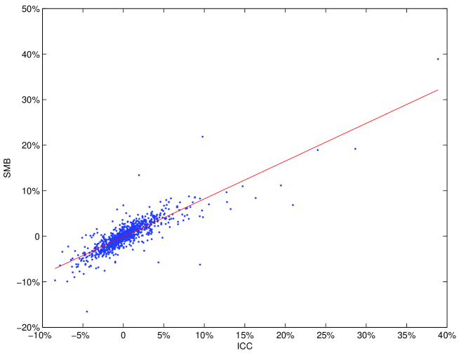
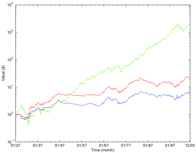
Figure 3: Comparison of ICC and SMB. The upper panel shows the return of the factor SMB versus the return of the factor ICC. The straight line shows the regression line with equation $y=-0.0008+0.8292\cdot x$. The lower panel depicts the value of $1 invested in the market portfolio in Jan. 1927 (grey curve; green online) and the value of a leveraged position of $1 invested in SMB (dark grey curve; blue online) and ICC (black curve; red online) in Jan. 1927. For the two arbitrage portfolios SMB and ICC, the initial endowment of $1 can be thought of as a reserve to ensure against risk losses, from which the returns can be discounted to provide the shown wealth curves.

The size effect is well-known to generally explain the part of the cross-section of expected returns left unexplained by any misspecified asset pricing model (?), which raises the question of its relevance as the signature of a genuine risk factor. Our theoretical model provides an answer to this question by rationalizing the role of the size effect as providing a proxy for the diversification factor $f$ (or ICC). Indeed, since the arbitrage portfolio which proxies the ICC factor is long in the equally-weighted portfolio and short in the market portfolio, it is therefore long on the small caps and short on the large caps, just like the SMB portfolio. There is thus no qualitative difference between the Fama and French’s factor SMB and our proxy of the ICC factor. This is confirmed by the large value of the linear correlation between the two portfolios proxying the SMB and ICC factors equal to 86% over the time interval studied here. As an illustration, the return on each factors is depicted on the left panel of figure 3 while the right panel represents the value of $1 invested in the market portfolio in Jan. 1927 and the value of a leveraged position of $1 invested in SMB and ICC in Jan. 1927.

[Insert figure 3 about here]

The book-to-market effect.

As illustrated by ? and ? in the early eighties and as emphasized more recently by ? (?, ?), stocks with a high book-to-market value tend to overperform stocks with a low book-to-market value. Several economic explanations have been proposed to justify this phenomenon. Among others, ? have proposed that value stocks are companies that are in financial distress while ? have suggested that growth stocks might have speculative investment opportunities that will be profitable only if equity financing is available on sufficiently good terms.

The pricing formula provided by proposition 3 offers a straightforward justification of the book-to-market effect. Indeed, there is good empirical evidence that high book-to-market stocks have significantly lower beta’s with respect to the market portfolio compared with low book-to-market stocks. For instance, using a large sample of firms from 1977 to 2004, ? find that the difference between the beta’s of growth opportunities and the beta’s of assets-in-place is positive and statistically significant, at the 95% level, in 34 out of 37 industry classifications. Bernardo et al. suggest that this results from the fact that, since firms with more growth opportunities have cash flows with longer duration, their values are more sensitive to changes in interest rates and thus should have higher beta’s. Then, ceteris paribus, the additional term $\left(\gamma_{i}-\gamma_{m}\cdot\beta_{i}\right)\cdot{\rm E}\left[r_{icc}-r_{0}\right]$ introduced by the internal consistency constraint leads to a higher expected rate of return for a stock with a low beta if the term $\gamma_{m}$ is positive.

4 Conclusion

Starting from a factorial model in which the only a priori systematic risk is the market portfolio, we have shown that there is a new source of significant systematic risk, which has been totally neglected up to now but which ought to be priced by the market. This occurs when (i) the internal consistency condition holds (which simply means that the market portfolio is constituted of the assets whose returns it is supposed to explain) and (ii) the distribution of the capitalization of firms is sufficiently fat-tailed, as is the case of real economies. The corresponding new internal consistent factors do not disappear for arbitrary large economies because the contribution, to the risk of arbitrary well-diversified portfolios due to the largest firms, remains finite for arbitrary large economies when the distribution of the capitalization of firms is sufficiently heavy-tailed. For this reason, this endogenous factor can be considered as related to the existence of a diversification/concentration premium resulting from the concern of investors with respect to the level of diversification of their portfolio in so far as holding the market portfolio alone does not allow for a good diversification.

Applied to the Arbitrage Pricing Theory, we have shown that the original derivation of Ross’ results still holds, provided that we explicitly include the additional diversification factor in the analysis. As a consequence, this factor is shown to provide possible theoretical economic explanations of some of the empirical factors reported in the literature. In particular, it allows understanding the superior performance of Fama and French three-factor model in explaining the cross section of stock returns. Indeed, the diversification factor provides a rationalization of the SMB factor as a proxy of this factor. Beside, being consistent with the fact that high book-to-market stocks have significantly lower beta’s with respect to the market portfolio compared with low book-to-market stocks, the Value/Growth effect is related to the increasing sensitivity of value stocks to the diversification factor. Finally, on the basis of only two factors (the market portfolio and the equally-weighted portfolio), our model turns out to be at least as successful as the Fama and French three-factor model in explaining the cross-section of monthly returns on US stock over the time period for Jan. 1927 to Dec 2005.

Table 1: Numerical simulations

Average, minimum and maximum value of the $R^{2}$ of the regression of the return of 20 equally weighted portfolios (randomly drawn from a market of $N=1000$ and $N=10000$ assets according to the model (19)) on the market portfolio ($r_{m}$), on the market portfolio and the internal consistency factor ($r_{m},f$), on the market portfolio and the (overall) equally weighted portfolio ($r_{m},r_{e}$), on the market portfolio and an under-diversified portfolio ($r_{m},r_{u}$) and on the market portfolio and a well-diversified arbitrage portfolios ($r_{m},r_{a}$). Different market situations are considered with distributions of firm sizes with tail index $\mu$ which varies from $0.5$ to $2$.

		N=1000						N=10000
		$r_{m}$	$r_{m},f$	$r_{m},r_{e}$	$r_{m},r_{u}$	$r_{m},r_{a}$		$r_{m}$	$r_{m},f$	$r_{m},r_{e}$	$r_{m},r_{u}$	$r_{m},r_{a}$
	Mean	94%	94%	95%	94%	94%		99%	99%	99%	99%	99%
$\mu=2$	Min	90%	93%	93%	90%	90%		99%	99%	99%	99%	99%
	Max	96%	96%	96%	96%	96%		100%	100%	100%	100%	100%
	Mean	80%	95%	95%	86%	82%		88%	99%	99%	93%	89%
$\mu=1$	Min	1%	91%	91%	42%	17%		20%	99%	99%	66%	20%
	Max	95%	100%	100%	95%	95%		99%	100%	100%	99%	99%
	Mean	56%	97%	97%	79%	64%		56%	100%	100%	83%	63%
$\mu=1/2$	Min	2%	89%	89%	34%	15%		1%	96%	97%	15%	3%
	Max	100%	100%	100%	100%	100%		100%	100%	100%	100%	100%

Table 2: Multi-factor time series regressions for monthly excess returns on 25 equally-weighted portfolios sorted by size and book-to-market (beta): Jan. 1927 - Dec. 2005, 948 months

Parameter estimates of the linear regression of the excess returns on 25 equally-weighed portfolios (sorted by quintiles of the distribution of size – Small, 2, 3, 4 and Big – and by quintiles of the distribution of Book equity to Market equity ratio – Low, 2, 3, 4 and High) regressed on the excess return on the market portfolio, on the two Fama-French factors SMB and HML and on the proxy for the additional risk factor due to the internal consistency constraint given by the difference between the return on the equally-weighted portfolio and the return on the market portfolio:

$$r_{i,t}-r_{0}=\alpha_{i}+\beta_{i}\cdot\left[r_{m}(t)-r_{0}\right]+\beta^{ICC}_{i}\cdot r_{icc}(t)+\beta^{SMB}_{i}\cdot r_{smb}(t)+\beta^{HML}_{i}\cdot r_{hml}(t)+\varepsilon_{i}(t).$$

In the four columns labeled $\beta$, $\beta^{SMB}$, $\beta^{HML}$ and $\beta^{ICC}$ the figures decorated by one star (resp. two stars) show the cases which reject the null hypothesis that the factor under consideration is not significant in the presence of the others at the 5% (resp. the 1%) level. For instance, for the portfolio Big-High, the factor SMB is not significant (neither at the 5% nor the 1% level) in the presence of both the market factor, the factor HML and the proxy for the factor ICC. Similarly, the factor ICC is not significant in the presence of the market factor, the SMB and HML factors while, in contrast, the factor HML is still significant at the $1\%$ level in the presence of the market factor, the the SMB and ICC factors.

		$\alpha$	$\beta$	$\beta^{SMB}$	$\beta^{HML}$	$\beta^{ICC}$	$R^{2}$
	Low	-0.0076	1.24∗∗	-0.49∗∗	-0.24∗∗	2.33∗∗	75%
	2	-0.0032	1.05∗∗	0.78∗∗	0.16∗	1.17∗∗	81%
Small	3	0.0007	1.01∗∗	0.37∗∗	0.21∗∗	1.06∗∗	89%
	4	0.0017	0.94∗∗	0.47∗∗	0.36∗∗	1.05∗∗	94%
	High	0.0037	0.93∗∗	0.45∗∗	0.65∗∗	1.32∗∗	92%
	Low	-0.0032	1.11∗∗	0.70∗∗	-0.38∗∗	0.56∗∗	90%
	2	-0.0009	1.11∗∗	0.69∗∗	0.14∗∗	0.34∗∗	94%
2	3	0.0011	0.98∗∗	0.75∗∗	0.33∗∗	0.20∗∗	93%
	4	0.0008	1.00∗∗	0.74∗∗	0.56∗∗	0.11∗∗	95%
	High	-0.0004	1.07∗∗	0.79∗∗	0.83∗∗	0.19∗∗	96%
	Low	-0.0021	1.16∗∗	0.29∗∗	-0.38∗∗	0.61∗∗	92%
	2	0.0010	1.03∗∗	0.44∗∗	0.03	0.11∗	92%
3	3	0.0005	1.04∗∗	0.38∗∗	0.32∗∗	0.08∗∗	93%
	4	0.0011	0.97∗∗	0.51∗∗	0.52∗∗	-0.01∗∗	93%
	High	-0.0007	1.18∗∗	0.31∗∗	0.87∗∗	0.28∗∗	94%
	Low	0.0004	1.08∗∗	0.07	-0.44∗∗	0.26∗∗	93%
	2	-0.0004	1.04∗∗	0.14∗∗	0.10∗∗	0.11∗	91%
4	3	0.0010	1.02∗∗	0.17∗∗	0.29∗∗	0.09	92%
	4	0.0002	1.08∗∗	0.08	0.57∗∗	0.16∗∗	93%
	High	-0.0024	1.27∗∗	0.17∗∗	0.98∗∗	0.28∗∗	93%
	Low	0.0002	1.06∗∗	-0.24∗∗	-0.35∗∗	0.21∗∗	96%
	2	0.0003	1.04∗∗	-0.19∗∗	0.07∗∗	0.13∗∗	94%
Big	3	-0.0001	1.04∗∗	-0.20∗∗	0.32∗∗	0.11∗∗	93%
	4	-0.0015	1.10∗∗	-0.30∗∗	0.66∗∗	0.26∗∗	92%
	High	-0.0012	1.10∗∗	-0.26∗∗	0.82∗∗	0.27∗∗	86%

Table 3: Multi-factor time series regressions for monthly excess returns on 25 equally-weighted portfolios sorted by size and book-to-market ($R^{2}$): Jan. 1927 - Dec. 2005, 948 months

$R^{2}$ of the linear regression of the excess returns of 25 equally-weighed portfolios (sorted by quintiles of the distribution of size – Small, 2, 3, 4 and Big – and by quintiles of the distribution of Book equity to Market equity ratio – Low, 2, 3, 4 and High) on the market portfolio (Rm), on the market portfolio and the factor ICC (ICC), on the market portfolio and the size factor (SMB), on the market portfolio and the book to market factor (HML), on the market portfolio and the two Fama&French factors (HML + SMB), on the market portfolio, the factor ICC and the size factor (ICC + SMB), on the market portfolio, the factor ICC and the book to market factor (ICC + HML) and, finally on all these four factors (Market, ICC, SMB and HML). Figures in boldface represent the maximum value of the $R^{2}$ within the group of regression with two factors (columns ICC, SMB and HML) and with three factors (columns HML + SMB, ICC + SMB and ICC + HML). The two last rows reports ? test statistics and $p$-values.

								HML	ICC	ICC		All
		Rm		ICC	SMB	HML		+	+	+		four
								SMB	SMB	HML		factors
	Low	52.0%		74.8%	66.7%	54.3%		68.6%	74.9%	74.8%		75.2%
		(43.1%,60.6%)		(68.5%,80.3%)	(60.1%,74.5%)	(44.3%,64.3%)		(62.1%,75.8%)	(68.7%,80.9%)	(69.3%,80.6%)		(69.6%,81.0%)
	2	51.8%		79.9%	76.4%	54.9%		78.9%	80.7%	79.9%		80.9%
		(43.4%,61.5%)		(73.0%,86.0%)	(71.9%,81.3%)	(45.7%,66.6%)		(73.3%,84.3%)	(75.1%,86.1%)	(74.0%,86.2%)		(75.5%,86.5%)
Small	3	63.8%		89.0%	82.9%	68.5%		87.0%	89.1%	89.1%		89.4%
		(57.2%,70.3%)		(85.8%,91.8%)	(80.0%,85.6%)	(60.7%,76.5%)		(83.9%,90.2%)	(86.4%,91.9%)	(85.8%,92.5%)		(86.6%,92.6%)
	4	61.7%		92.5%	84.4%	69.4%		91.3%	92.6%	93.2%		93.7%
		(53.8%,69.8%)		(90.9%,94.2%)	(81.6%,87.6%)	(62.1%,77.2%)		(89.3%,93.2%)	(91.0%,94.3%)	(91.7%,95.0%)		(92.5%,95.3%)
	High	53.9%		89.5%	77.2%	67.5%		89.6%	89.7%	92.1%		92.5%
		(46.3%,62.6%)		(86.0%,92.5%)	(71.2%,82.5%)	(60.9%,74.3%)		(85.9%,92.4%)	(86.1%,92.7%)	(89.5%,94.4%)		(89.9%,94.8%)
	Low	70.3%		84.2%	88.9%	70.8%		89.6%	88.9%	89.0%		90.4%
		(66.1%,75.4%)		(81.0%,87.7%)	(86.1%,91.5%)	(66.5%,76.3%)		(87.1%,92.1%)	(86.4%,91.5%)	(86.7%,91.5%)		(88.5%,92.6%)
	2	78.0%		92.2%	92.3%	79.3%		93.4%	93.5%	92.3%		93.7%
		(71.3%,84.1%)		(90.3%,94.1%)	(90.8%,94.0%)	(73.2%,85.0%)		(92.1%,94.9%)	(92.3%,95.0%)	(90.5%,94.2%)		(92.5%,95.2%)
2	3	74.6%		90.8%	89.6%	78.4%		92.9%	91.6%	91.1%		93.0%
		(65.9%,83.0%)		(88.3%,93.8%)	(86.9%,92.8%)	(71.0%,85.9%)		(91.2%,95.3%)	(89.5%,94.2%)	(88.8%,94.1%)		(91.4%,95.4%)
	4	75.8%		91.0%	87.7%	83.6%		94.9%	91.1%	93.2%		95.0%
		(69.2%,81.8%)		(88.4%,93.1%)	(84.7%,90.7%)	(78.5%,88.5%)		(93.7%,96.2%)	(88.6%,93.2%)	(91.4%,94.8%)		(93.8%,96.2%)
	High	71.3%		89.3%	83.4%	84.4%		95.8%	89.4%	94.3%		95.9%
		(65.5%,76.6%)		(85.7%,92.0%)	(79.3%,87.5%)	(80.4%,88.0%)		(94.0%,97.0%)	(85.8%,92.0%)	(92.2%,95.8%)		(94.2%,97.1%)
												(continued)

Table 4: Continued

								HML	ICC	ICC		All
		Rm		ICC	SMB	HML		+	+	+		four
								SMB	SMB	HML		factors
	Low	80.3%		88.6%	90.7%	80.8%		91.4%	90.8%	92.2%		92.5%
		(75.7%,84.8%)		(86.1%,90.8%)	(87.8%,93.0%)	(76.5%,85.5%)		(88.9%,93.5%)	(88.4%,93.1%)	(90.6%,93.7%)		(90.9%,94.0%)
	2	85.6%		90.9%	91.8%	85.7%		92.0%	92.0%	91.1%		92.0%
		(82.7%,88.3%)		(89.1%,92.9%)	(89.7%,93.8%)	(82.9%,88.6%)		(90.1%,93.9%)	(90.1%,93.9%)	(89.2%,93.0%)		(90.2%,93.9%)
3	3	85.4%		91.4%	89.9%	88.8%		93.0%	91.4%	92.4%		93.1%
		(81.9%,88.4%)		(89.2%,93.2%)	(87.3%,92.1%)	(86.3%,90.9%)		(91.5%,94.3%)	(89.3%,93.3%)	(90.8%,93.8%)		(91.5%,94.3%)
	4	80.4%		88.7%	86.0%	87.8%		93.0%	88.7%	91.9%		93.0%
		(75.2%,84.9%)		(85.0%,91.6%)	(82.2%,89.4%)	(84.3%,91.1%)		(91.1%,94.7%)	(85.2%,91.7%)	(89.6%,93.9%)		(91.1%,94.7%)
	High	75.6%		85.9%	79.9%	90.5%		94.3%	87.2%	94.2%		94.4%
		(70.8%,79.7%)		(82.5%,88.9%)	(75.8%,83.9%)	(87.1%,93.1%)		(92.4%,95.8%)	(83.7%,90.3%)	(92.0%,95.8%)		(92.6%,96.0%)
	Low	86.4%		87.0%	88.4%	90.2%		92.3%	89.0%	92.6%		92.6%
		(84.0%,88.7%)		(84.8%,89.3%)	(86.2%,90.4%)	(88.3%,91.8%)		(90.8%,93.7%)	(86.9%,91.2%)	(91.4%,93.9%)		(91.4%,94.0%)
	2	89.4%		91.3%	90.8%	90.0%		91.4%	91.3%	91.4%		91.5%
		(87.1%,91.5%)		(89.0%,93.3%)	(88.2%,93.1%)	(88.0%,91.9%)		(89.3%,93.5%)	(89.1%,93.4%)	(89.3%,93.4%)		(89.4%,93.5%)
4	3	87.3%		90.3%	88.9%	90.5%		92.0%	90.5%	91.9%		92.0%
		(84.5%,89.8%)		(87.5%,92.5%)	(86.2%,91.5%)	(88.5%,92.6%)		(89.8%,94.0%)	(87.8%,92.7%)	(89.7%,93.8%)		(89.8%,94.0%)
	4	82.5%		86.6%	83.5%	91.8%		92.7%	88.1%	92.8%		92.8%
		(78.6%,85.7%)		(82.6%,89.8%)	(79.9%,87.1%)	(89.2%,93.9%)		(90.3%,94.6%)	(84.1%,91.1%)	(90.2%,94.6%)		(90.3%,94.7%)
	High	74.4%		82.1%	76.6%	90.7%		92.5%	84.5%	92.6%		92.7%
		(69.6%,78.9%)		(77.6%,85.9%)	(72.0%,81.1%)	(87.6%,93.2%)		(89.9%,94.5%)	(79.7%,88.7%)	(90.0%,94.6%)		(90.1%,94.6%)
	Low	92.0%		92.5%	92.2%	95.1%		95.2%	92.7%	95.1%		95.5%
		(90.5%,93.3%)		(91.0%,93.8%)	(90.7%,93.5%)	(94.0%,96.1%)		(94.2%,96.2%)	(91.1%,94.1%)	(94.0%,96.1%)		(94.6%,96.4%)
	2	93.3%		93.3%	93.5%	93.7%		93.9%	93.9%	93.7%		94.0%
		(91.0%,94.9%)		(91.0%,95.0%)	(91.5%,95.0%)	(91.6%,95.3%)		(92.0%,95.4%)	(92.1%,95.4%)	(91.8%,95.3%)		(92.2%,95.5%)
Big	3	88.2%		88.3%	88.4%	92.3%		92.7%	90.6%	92.5%		92.7%
		(85.0%,90.6%)		(85.1%,90.9%)	(85.6%,90.9%)	(90.0%,94.2%)		(90.5%,94.5%)	(87.9%,93.0%)	(90.3%,94.3%)		(90.5%,94.6%)
	4	79.0%		80.5%	79.1%	91.9%		92.0%	86.0%	91.9%		92.2%
		(74.3%,82.9%)		(75.8%,84.5%)	(74.7%,83.0%)	(89.2%,94.0%)		(89.3%,94.1%)	(81.5%,89.6%)	(89.2%,94.0%)		(89.6%,94.3%)
	High	70.1%		72.6%	70.1%	86.2%		86.2%	78.5%	86.3%		86.5%
		(64.1%,75.2%)		(66.9%,77.2%)	(64.4%,75.3%)	(82.4%,89.9%)		(82.5%,89.9%)	(72.7%,83.3%)	(82.5%,89.9%)		(82.8%,90.1%)
Average		76.1%		87.3%	84.7%	82.2%		90.6%	88.6%	90.8%		91.4%
		(72.6%,79.7%)		(85.3%,89.3%)	(82.4%,87.2%)	(79.4%,85.3%)		(89.1%,92.2%)	(86.7%,90.6%)	(89.5%,92.2%)		(90.2%,92.8%)
GRS		4.37		4.11	4.41	4.02		4.07	4.19	3.92		4.06
p-value		0.00		0.00	0.00	0.00		0.00	0.00	0.00		0.00

Table 5: Multi-factor time series regressions for monthly excess returns on 10 value-weighted industry portfolios (beta): Jan. 1927 - Dec. 2005, 948 months

Parameter estimates of the linear regression of the excess returns of ten value-weighed industry portfolios regressed on the excess return on the market portfolio, on the two Fama-French factors SMB and HML and on the proxy for the additional risk factor due to the internal consistency constraint given by the difference between the return on the equally-weighted portfolio and the return on the market portfolio:

$$r_{i,t}-r_{0}=\alpha_{i}+\beta_{i}\cdot\left[r_{m}(t)-r_{0}\right]+\beta^{ICC}_{i}\cdot r_{icc}(t)+\beta^{SMB}_{i}\cdot r_{smb}(t)+\beta^{HML}_{i}\cdot r_{hml}(t)+\varepsilon_{i}(t).$$

In the four columns labeled $\beta$, $\beta^{SMB}$, $\beta^{HML}$ and $\beta^{ICC}$, the figures decorated by one star (resp. two stars) show the cases which reject the null hypothesis that the factor under consideration is not significant in the presence of the others at the 5% (resp. the 1%) level. For instance, for the Shops, the Health and the Utilities industries, the factor SMB is not significant (neither at the 5% nor the 1% level) in the presence of both the market factor, the factor HML and the proxy for the factor ICC. Similarly, for the same industry portfolio, the factor ICC is not significant in the presence of the market factor and the SMB and HML factors.

Industry	$\alpha$	$\beta$	$\beta^{SMB}$	$\beta^{HML}$	$\beta^{ICC}$	$R^{2}$
Consumer Non Durables	0.0019	0.78∗∗	0.08	0.07∗	-0.15∗∗	78%
Consumer Durables	-0.0006	1.11∗∗	-0.12	0.11∗	0.24∗∗	75%
Manufacturing	-0.0006	1.10∗∗	0.11∗∗	0.19∗∗	-0.11∗	92%
Energy	0.0018	0.86∗∗	-0.10	0.30∗∗	-0.16	64%
Business Equipment	0.0012	1.27∗∗	-0.21∗∗	-0.45∗∗	0.37∗∗	84%
Telecom	0.0015	0.69∗∗	-0.27∗∗	-0.15∗∗	0.18∗∗	63%
Shops	0.0010	0.96∗∗	0.03	-0.14∗∗	0.06	80%
Health	0.0030	0.91∗∗	-0.01	-0.15∗∗	-0.11	68%
Utilities	-0.0001	0.79∗∗	-0.05	0.35∗∗	-0.11	63%
Others	-0.0016	1.06∗∗	-0.07	0.30∗∗	0.12∗∗	92%

Table 6: Multi-factor time series regressions for monthly excess returns on 10 value-weighted industry portfolios ($R^{2}$): Jan. 1927 - Dec. 2005, 948 months

$R^{2}$ of the linear regressions of the excess returns of ten value-weighed industry portfolios regressed on the (excess return) on the market portfolio (Rm), on the market portfolio and the factor ICC (ICC), on the market portfolio and the size factor (SMB), on the market portfolio and the book to market factor (HML), on the market portfolio and the two Fama&French factors (HML + SMB), on the market portfolio, the factor ICC and the size factor (ICC + SMB), on the market portfolio, the factor ICC and the book to market factor (ICC + HML) and, finally on the four factors (market, ICC, SMB, HML). Figures in boldface represent the maximum value of the $R^{2}$ within the group of regressions with two factors (columns ICC, SMB and HML) and with three factors (columns HML + SMB, ICC + SMB and ICC + HML). The two last rows reports ? test statistics and $p$-values.

							HML	ICC	ICC		All
	Rm		ICC	SMB	HML		+	+	+		four
							SMB	SMB	HML		factors
Consumer Non Durables	77.4%		77.6%	77.5%	77.5%		77.5%	77.6%	77.7%		77.7%
	(72.6%,81.4%)		(72.8%,81.7%)	(72.7%,81.5%)	(72.8%,81.6%)		(73.0%,81.7%)	(72.9%,81.7%)	(73.0%,81.7%)		(73.1%,81.9%)
Consumer Durables	74.0%		74.6%	74.2%	74.8%		74.9%	75.0%	75.1%		75.1%
	(69.0%,78.4%)		(69.8%,78.9%)	(69.2%,78.5%)	(69.9%,79.2%)		(70.1%,79.3%)	(70.2%,79.4%)	(70.3%,79.4%)		(70.4%,79.5%)
Manufacturing	91.6%		91.7%	91.6%	92.3%		92.3%	91.7%	92.3%		92.4%
	(89.6%,93.2%)		(89.7%,93.4%)	(89.6%,93.3%)	(90.5%,93.8%)		(90.5%,93.8%)	(89.8%,93.5%)	(90.5%,93.8%)		(90.6%,93.9%)
Energy	60.1%		60.4%	61.4%	62.2%		63.6%	61.9%	63.7%		63.7%
	(53.9%,65.3%)		(54.2%,65.8%)	(55.5%,66.7%)	(56.0%,67.2%)		(58.2%,68.6%)	(56.0%,67.2%)	(58.2%,68.6%)		(58.3%,68.7%)
Business Equipment	81.3%		81.3%	81.4%	83.6%		83.8%	81.6%	84.0%		84.2%
	(77.3%,84.6%)		(77.5%,84.6%)	(77.9%,84.7%)	(80.7%,86.2%)		(80.9%,86.4%)	(78.1%,84.9%)	(81.3%,86.6%)		(81.6%,86.8%)
Telecom	61.4%		62.0%	62.2%	62.0%		62.7%	62.2%	62.3%		63.0%
	(56.0%,66.5%)		(57.2%,67.0%)	(57.3%,67.2%)	(56.9%,67.0%)		(58.1%,67.6%)	(57.5%,67.3%)	(57.6%,67.2%)		(58.5%,67.9%)
Shops	78.9%		78.9%	79.1%	79.4%		79.5%	79.2%	79.6%		79.6%
	(74.5%,82.7%)		(74.6%,82.7%)	(74.8%,83.1%)	(75.3%,83.1%)		(75.5%,83.4%)	(75.0%,83.2%)	(75.5%,83.3%)		(75.6%,83.4%)
Health	66.0%		67.0%	66.4%	67.3%		67.7%	67.2%	67.7%		67.7%
	(59.1%,71.3%)		(60.8%,72.4%)	(59.8%,71.7%)	(61.0%,72.5%)		(61.6%,72.9%)	(61.5%,72.7%)	(61.8%,73.1%)		(62.2%,73.2%)
Utilities	58.5%		58.5%	59.1%	62.2%		62.9%	60.1%	62.9%		62.9%
	(51.0%,65.3%)		(51.0%,65.5%)	(51.8%,65.6%)	(55.3%,68.7%)		(56.1%,69.1%)	(52.9%,66.8%)	(56.4%,69.2%)		(56.5%,69.2%)
Others	88.4%		89.2%	88.4%	91.7%		91.7%	90.2%	91.8%		91.8%
	(86.5%,90.2%)		(87.2%,91.1%)	(86.5%,90.4%)	(89.9%,93.6%)		(89.9%,93.6%)	(88.4%,92.2%)	(90.0%,93.6%)		(90.0%,93.7%)
Average	73.7%		74.1%	74.1%	75.2%		75.6%	74.6%	75.6%		75.7%
	(70.2%,76.8%)		(70.8%,77.2%)	(70.8%,77.2%)	(72.1%,78.2%)		(72.7%,78.6%)	(71.4%,77.8%)	(72.6%,78.6%)		(72.9%,78.7%)
GRS	2.67		3.23	3.16	3.32		3.69	3.09	3.63		3.65
$p$-value	0.00		0.00	0.00	0.00		0.00	0.00	0.00		0.00

Table 7: Multi-factor time series regressions for monthly excess returns on 10 equally-weighted industry portfolios (beta): Jan. 1927 - Dec. 2005, 948 months

Parameter estimates of the linear regression of the excess returns of ten equally-weighed industry portfolios regressed on the excess return on the market portfolio, on the two Fama-French factors SMB and HML and on the proxy for the additional risk factor due to the internal consistency constraint given by the difference between the return on the equally-weighted portfolio and the return on the market portfolio:

$$r_{i,t}-r_{0}=\alpha_{i}+\beta_{i}\cdot\left[r_{m}(t)-r_{0}\right]+\beta^{ICC}_{i}\cdot r_{icc}(t)+\beta^{SMB}_{i}\cdot r_{smb}(t)+\beta^{HML}_{i}\cdot r_{hml}(t)+\varepsilon_{i}(t).$$

In the four columns labeled $\beta$, $\beta^{SMB}$, $\beta^{HML}$ and $\beta^{ICC}$, the figures decorated by one star (resp. two stars) show the cases which reject the null hypothesis that the factor under consideration is not significant in the presence of the others at the 5% (resp. the 1%) level.

Industry	$\alpha$	$\beta$	$\beta^{SMB}$	$\beta^{HML}$	$\beta^{ICC}$	$R^{2}$
Consumer Non Durables	-0.0003	0.84∗∗	0.08∗	0.10∗∗	0.77∗∗	94%
Consumer Durables	-0.0024	1.12∗∗	0.21∗∗	0.07∗	0.97∗∗	92%
Manufacturing	-0.0004	1.07∗∗	0.12∗∗	0.17∗∗	0.76∗∗	97%
Energy	0.0019	0.95∗∗	0.13	0.34∗∗	0.55∗∗	69%
Business Equipment	0.0016	1.22∗∗	-0.29∗∗	-0.65∗∗	1.52∗∗	92%
Telecom	0.0030	0.92∗∗	-0.30∗∗	-0.54∗∗	0.98∗∗	73%
Shops	0.0000	0.91∗∗	0.11∗	-0.11∗∗	0.93∗∗	90%
Health	0.0037	0.91∗∗	-0.04	-0.54∗∗	0.92∗∗	80%
Utilities	0.0006	0.85∗∗	0.21∗	0.55∗∗	-0.06	66%
Others	-0.0008	0.95∗∗	0.07	0.39∗∗	0.93∗∗	95%

Table 8: Multi-factor time series regressions for monthly excess returns on 10 equally-weighted industry portfolios ($R^{2}$): Jan. 1927 - Dec. 2005, 948 months

$R^{2}$ of the linear regression of the excess returns of ten equally-weighed industry portfolios regressed on the (excess return) on the market portfolio (Rm), on the market portfolio and the factor ICC (ICC), on the market portfolio and the size factor (SMB), on the market portfolio and the book to market factor (HML), on the market portfolio and the two Fama&French factors (HML + SMB), on the market portfolio, the factor ICC and the size factor (ICC + SMB), on the market portfolio, the factor ICC and the book to market factor (ICC + HML) and, finally on the four factors (market, ICC, SMB and HML). Figures in boldface represent the maximum value of the $R^{2}$ within the group of regression with two factors (columns ICC, SMB and HML) and with three factors (columns HML + SMB, ICC + SMB and ICC + HML). The two last rows reports ? test statistics and $p$-values.

							HML	ICC	ICC		All
	Rm		ICC	SMB	HML		+	+	+		four
							SMB	SMB	HML		factors
Consumer Non Durables	75.9%		94.1%	88.4%	79.7%		91.8%	94.1%	94.3%		94.3%
	(70.9%,80.5%)		(92.4%,95.5%)	(85.2%,91.2%)	(74.9%,83.9%)		(89.5%,93.9%)	(92.5%,95.5%)	(92.7%,95.6%)		(92.7%,95.7%)
Consumer Durables	74.4%		92.3%	87.9%	76.9%		90.2%	92.4%	92.3%		92.4%
	(69.2%,79.2%)		(90.2%,94.2%)	(84.8%,91.1%)	(72.2%,81.9%)		(87.6%,92.6%)	(90.3%,94.3%)	(90.2%,94.2%)		(90.4%,94.3%)
Manufacturing	82.2%		96.7%	92.0%	85.9%		95.4%	96.8%	97.0%		97.1%
	(78.3%,86.0%)		(95.7%,97.6%)	(89.9%,93.9%)	(82.5%,88.9%)		(93.9%,96.6%)	(95.7%,97.6%)	(96.1%,97.8%)		(96.2%,97.9%)
Energy	58.3%		67.8%	63.7%	63.4%		68.5%	68.1%	69.3%		69.3%
	(51.7%,64.5%)		(61.9%,73.7%)	(57.6%,69.9%)	(58.6%,68.5%)		(63.0%,74.1%)	(62.3%,74.0%)	(64.0%,74.7%)		(64.0%,74.8%)
Business Equipment	74.5%		87.4%	86.2%	74.8%		86.6%	88.0%	91.6%		91.8%
	(68.7%,79.9%)		(85.0%,89.8%)	(82.5%,89.4%)	(69.3%,80.1%)		(83.2%,89.6%)	(85.9%,90.4%)	(90.1%,93.0%)		(90.4%,93.2%)
Telecom	62.7%		68.2%	68.1%	63.9%		69.4%	68.6%	72.6%		73.0%
	(55.4%,69.2%)		(64.0%,72.8%)	(61.4%,74.0%)	(56.5%,70.5%)		(63.4%,75.1%)	(64.2%,74.2%)	(69.0%,77.0%)		(69.5%,77.3%)
Shops	71.8%		90.1%	86.7%	72.8%		87.6%	90.3%	90.4%		90.5%
	(66.7%,77.0%)		(86.2%,93.1%)	(82.8%,90.5%)	(67.7%,78.2%)		(83.6%,91.2%)	(86.6%,93.4%)	(87.1%,93.3%)		(87.1%,93.4%)
Health	65.1%		74.5%	75.9%	66.4%		77.4%	76.2%	80.5%		80.5%
	(58.2%,71.3%)		(69.5%,79.0%)	(72.0%,79.7%)	(60.0%,72.5%)		(73.7%,81.0%)	(72.8%,79.9%)	(77.3%,83.7%)		(77.4%,83.8%)
Utilities	58.3%		60.8%	58.9%	65.9%		66.5%	61.7%	66.3%		66.5%
	(51.0%,65.3%)		(52.8%,68.8%)	(51.6%,66.8%)	(58.2%,72.8%)		(58.3%,74.0%)	(53.8%,69.5%)	(58.3%,73.6%)		(58.5%,74.1%)
Others	71.9%		92.8%	83.6%	81.6%		92.7%	93.4%	95.2%		95.2%
	(66.1%,77.2%)		(90.5%,94.8%)	(79.3%,87.5%)	(77.5%,85.3%)		(90.1%,94.9%)	(91.1%,95.3%)	(93.4%,96.6%)		(93.5%,96.6%)
Average	69.5%		82.4%	79.1%	73.1%		82.6%	82.9%	84.9%		85.0%
	(65.0%,73.9%)		(79.9%,85.1%)	(76.0%,82.3%)	(69.0%,77.1%)		(79.9%,85.4%)	(80.5%,85.6%)	(82.9%,87.2%)		(83.0%,87.3%)
GRS	2.53		2.21	2.69	2.72		2.61	2.24	2.70		2.70
$p$-value	0.01		0.02	0.00	0.00		0.00	0.01	0.00		0.00

References

- [1]
- [2] [] Abramowitz, Milton, and Irene A. Stegun, 1972, Handbook of Mathematical Functions (Dover Publications).
- [3]
- [4] [] Alexander, Gordon J., and Alexandre M. Baptista, 2002, Economic implications of using a mean-VaR model for portfolio selection: A comparison with mean-variance analysis, Journal of Economic Dynamics & Control 26, 1159-1193.
- [5]
- [6] [] Alexander, Gordon J., and Jack C. Francis, 1986, Portfolio Analysis (Prentice Hall).
- [7]
- [8] [] Axtell, Robert L., 2001, Zipf distribution of U.S. firm sizes, Science 293, 1818-1820.
- [9]
- [10] [] Axtell, Robert L., 2006, Firm sizes: facts, formulae, fables and fantasies, in Claudio Cioffi-Revilla, ed.: Power Laws in the Social Sciences (Cambridge University Press). Forthcoming.
- [11]
- [12] [] Bain, Joe S., 1956, Barriers to New Competition: Their Character and Consequences in Manufacturing Industries ( A. M. Kelley, Reprint edition, September 1993).
- [13]
- [14] [] Banz, Rolf W., 1981, The relationship between return and market values of common stocks, Journal of Financial Economics 9, 3-18.
- [15]
- [16] [] Basu, S., 1977, Investment performance of common stocks in relation to their price-earning ratios: A test of the efficient market hypothesis, Journal of Finance 32, 663-682.
- [17]
- [18] [] Berk, Jonathan B., 1995, A critique of size-related anomalies, Review of Financial Studies 8, 275-286.
- [19]
- [20] [] Bernardo, Antonio E., Bhagwan Chowdry, and Amit Goyal, 2007, Growth Options, Beta, and the Cost of Capital, Financial Management, forthcoming.
- [21]
- [22] [] Bingham, Nicholas H., Charles M. Goldie and Jozef L. Teugels, 1987, Regular Variation (Cambridge University Press).
- [23]
- [24] [] Blume, Marshall E., 1980, Stock returns and dividend yields: some more evidence, Review of Economics and Statistics 62, 567 577.
- [25]
- [26] [] Bodie, Zvi , 1976, Common Stocks as a Hedge Against Inflation, Journal of Finance 31, 459-470.
- [27]
- [28] [] Burmeister, Edwin, and Kent D. Wall, 1986, The arbitrage pricing theory and macroeconomic factor measures, The Financial Review 21, 1-20.
- [29]
- [30] [] Campbell, John Y., and Tuomo Vuolteenaho, 2004, Bad beta, good beta, American Economic Review 94, 1249-1275.
- [31]
- [32] [] Campbell, John Y., Christopher Polk and Tuomo Vuolteenaho, 2005, Growth or Glamour? Fundamentals and Systematic Risk in Stock Returns, NBER Working Paper No. 11389, http://papers.nber.org/papers/w11389
- [33]
- [34] [] Chamberlain, Gary, 1983, Funds, factors and diversification in arbitrage pricing theory, Econometrica 51, 1305-1324.
- [35]
- [36] [] Chamberlain, Gary and Michael Rothschild, 1983, Arbitrage, factor structure, and mean-variance analysis on large asset markets, Econometrica 51, 1281-1304.
- [37]
- [38] [] Chan, Louis K.C., Narasimhan Jegadeesh, and Josef Lakonishok, 1996, Momentum Strategies, Journal of Finance 51, 1681-1713.
- [39]
- [40] [] Chan, Louis K.C., 1988, On the contrarian investment strategy, Journal of Business 61, 147-163
- [41]
- [42] [] Chen Nai-Fu, Richard Roll and Stephen A. Ross, 1986, Economic forces and the stock market, Journal of Business 59, 383-403.
- [43]
- [44] [] Chopra, Navin, Josef Lakonishok and Jay R. Ritter, 1992, Measuring abnormal performance : Do stocks overreact? Journal of Financial Economics 31, 235-268
- [45]
- [46] [] Connor, Gregory, 1982, Asset pricing in factor economies, Doctoral dissertation (Yale university).
- [47]
- [48] [] Cutler, David M., James M. Poterba and Lawrence H. Summers,1989 ,What Moves Stock Prices?, Journal of Portfolio Management 15, 4-12.
- [49]
- [50] [] Daniel, Kent D., David A. Hirshleifer and Avanidhar Subrahmanyam, 2001, Covariance risk, mispricing, and the cross-section of security returns, Journal of Finance 56, 921-965.
- [51]
- [52] [] Darling, D. A., 1952, The influence of the maximum term in the addition of independent random variables, Transactions of the American Mathematical Society 73, 95-107.
- [53]
- [54] [] DeBondt, Werner F. M., and Richard H. Thaller, 1985, Does the stock market overreact, Journal of Finance 40, 793-805.
- [55]
- [56] [] DeBondt, Werner F. M., and Richard H. Thaller, 1987, Further evidence on investor overreaction and stock market seasonality, Journal of Finance 42, 557-581.
- [57]
- [58] [] Dybvig, Philip H., 1983, An explicit bound on individual assets’ deviations from ATP pricing in a finite economy, Journal of Financial Economics 12, 483-496.
- [59]
- [60] [] Efron, Bradley, and Robert J. Tibshirani, 1993, An Introduction to the Bootstrap (Chapman & Hall, CRC).
- [61]
- [62] [] Embrechts, Paul, Claudia Klueppelberg and Thomas Mikosch, 1997, Modelling Extremal Events for Insurance and Finance (Springer-Verlag, Heidelberg)
- [63]
- [64] [] Fama, Eugene F., 1973, A Note on the Market Model and the Two-Parameter Model, Journal of Finance 28, 1181-1185.
- [65]
- [66] [] Fama, Eugene F., 1981, Stock returns, inflation and money, American Economic Review 71, 545-565.
- [67]
- [68] [] Fama, Eugene. F., and Kenneth R. French, 1992, The Cross-Section of Expected Stock Returns, Journal of Finance 47, 427-465.
- [69]
- [70] [] Fama, Eugene. F., and Kenneth R. French, 1993, Common Risk Factors in the Returns on Stocks and Bonds, Journal of Financial Economics 33, 3-56.
- [71]
- [72] [] Fama, Eugene. F., and Kenneth R. French, 1995, Size and Book-to-Market Factors in Earnings and Returns, Journal of Finance 50, 131-155.
- [73]
- [74] [] Fama, Eugene. F., and Kenneth R. French, 1996, Multifactor explanations of asset pricing anomalies, Journal of Finance 51, 55-84.
- [75]
- [76] [] Feller, William, 1971, An Introduction to Probability Theory and its Applications (Wiley).
- [77]
- [78] [] Ferson Wayne E. and Campbell R. Harvey, 1993, The Risk and Predictability of International Equity Returns, Review of Financial Studies 6, 527-566.
- [79]
- [80] [] Flannery, Mark J., and Aris A. Protopapadakis, 2002, Macroeconomic factors do influence aggregate stock returns, Review of Financial Studies 15, 751-782.
- [81]
- [82] [] Gabaix, Xavier, 1999a, Zipf’s Law and the Growth of Cities, American Economic Review 89, 129-132.
- [83]
- [84] [] Gabaix, Xavier, 1999b, Zipf’s Law For Cities: An Explanation, Quarterly Journal of Economics 114, 739-767.
- [85]
- [86] [] Gabaix, Xavier, 2005, The Granular Origins of Aggregate Fluctuations, Working Paper, MIT.
- [87]
- [88] [] Gabaix, Xavier, and Yannis Ioannides, 2004, The evolution of the city size distribution, in V. Henderson and J. Thisse ed.: Handbook of Urban and Regional Economics, Vol. 4 (North Holland).
- [89]
- [90] [] Gabaix, Xavier, Parameswaran Gopikrishnan, Vasiliki Plerou, H. Eugene Stanley, 2006, Institutional Investors and Stock Market Volatility, Quarterly Journal of Economics 121, 461-504.
- [91]
- [92] [] Geske, Robert and Richard Roll, 1983, The Fiscal and Monetary Linkage Between Stock Returns and Inflation, Journal of Finance 38, 1-33.
- [93]
- [94] [] Gibrat, Robert, 1931, Les Inégalitiés Economiques; Applications aux inégalitiés des richesses, à la concentration des entreprises, aux populations des villes, aux statistiques des familles, etc., d’une loi nouvelle, la loi de l’effet proportionnel (Librarie du Recueil Sirey, Paris).
- [95]
- [96] [] Gibbons, Michael R., Stephen A. Ross and Jay Shanken, 1989, A test of the efficiency of a given portfolio, Econometrica 57, 1121-1152.
- [97]
- [98] [] Gnedenko, Boris V. and Andrey N. Kolmogorov, 1954, Limit Distributions for Sums of Independent Random Variables (Addison-Wesley).
- [99]
- [100] [] Grinblatt, Mark, and Sheridan Titman, 1983, Factor pricing in a finite economy, Journal of Financial Economics 12, 497-507.
- [101]
- [102] [] Grinblatt, Mark, and Sheridan Titman, 1983, Approximate factor structures: Interpretations and implications for empirical tests, Journal of Finance 40, 1367-1373.
- [103]
- [104] [] Harvey, Campbell R., 1991, The world price of covariance risk, Journal of Finance 46, 111-157.
- [105]
- [106] [] Harvey, Campbell R. and Akhtar Siddique, 2000, Conditional skewness in asset pricing tests, Journal of Finance 55, 1263-1295.
- [107]
- [108] [] Huberman, Gur , 1982, A simple approach to arbitrage pricing theory, Journal of Economic Theory 28, 183-191.
- [109]
- [110] [] Ibragimov, I. A. and Yu V. Linnik, 1975, Independent and Stationary Sequences of Random Variables (Wolters-Noordhoff).
- [111]
- [112] [] Ijri, Yuji, and Herbert A. Simon, 1977, Skew Distribution of Sizes of Business Firms (North-Holland, Amsterdam).
- [113]
- [114] [] Ingersoll, Jonathan E., 1984, Some results in the theory of arbitrage pricing, Journal of Finance 39, 1021-1039.
- [115]
- [116] [] Jagannathan, Ravi and Zhenyu Wang, 1996, The conditional CAPM and the cross-section of expected returns, Journal of Finance 51, 3 53.
- [117]
- [118] [] Jagannathan, Ravi and Yong Wang, 2007, Lazy investors, discretionary consumption, and the cross-section of stock returns, Journal of Finance Forthcoming.
- [119]
- [120] [] Jegadeesh, Narasimhan, and Sheridan Titman, 1993, Returns to buying winners and selling losers: Implications for stock market efficiency, Journal of Finance 48, 65-91.
- [121]
- [122] [] Jegadeesh, Narasimhan, and Sheridan Titman, 2001, Profitability of Momentum Strategies: An Evaluation of Alternative Explanations, Journal of Finance 56, 699 720.
- [123]
- [124] [] Jones, Charles M. and Gautam Kaul, 1996, Oil and the Stock Markets, Journal of Finance 51, 463-491.
- [125]
- [126] [] Keim, Donald B., 1985, Dividend yields and stock returns, Journal of Financial Economics 14, 473 489.
- [127]
- [128] [] King, Benjamin F., 1966, Market and Industry Factors in Stock Price Behavior, Journal of Business 39, 139-170.
- [129]
- [130] [] Krauss, Alan, and Robert H. Litzenberger, 1976, Skewness preference and the valuation of risk assets, Journal of Finance 31, 1085-1099.
- [131]
- [132] [] Lakonishok, Joseph, Andrei Shleifer, and Robert W. Vishny, 1994, Contrarian investment extrapolation and risk, Journal of Finance 49, 1541-1578.
- [133]
- [134] [] Lovett, William A., 1988, Banking and Financial Institutions Law in a Nutshell (Second Edition, West Publishing Co.).
- [135]
- [136] [] Lim, Kian-Guan, 1989, A new test for the three-moment capital asset pricing model, Journal of Financial & Quantitative Analysis 24, 205-216.
- [137]
- [138] [] Lintner, John, 1965, The valuation of risk assets and the selection of risky investments in stock portfolios and capital budgets, Review of Economics and Statistics 47, 13-37.
- [139]
- [140] [] Logan, B. F., C. L. Mallows, S. O. Rice and L. A. Shepp, 1973, Limit distribution of self-normalized sums, Annals of Probability 1, 788-809.
- [141]
- [142] [] Lucas, Robert E., 1978, On the distribution of business firms, Bell Journal of Economics 9, 508-523.
- [143]
- [144] [] Marsili, Orietta, 2005, Technology and the Size Distribution of Firms: Evidence from Dutch Manufacturing, Review of Industrial Organization 27, 303-328.
- [145]
- [146] [] Meerschaert, Mark M. and Hans-Peter Scheffler, 2001, Limit Distributions for Sums of Independent Random Vectors: Heavy Tails in Theory and Practice (Wiley).
- [147]
- [148] [] Mosimann, James E., 1962, On the compound multinomial distribution, the -distribution and the correlations among proportions, Biometrika 49, 65-82.
- [149]
- [150] [] Mossin, Jan, 1966, Equilibrium in a Capital Asset Market, Econometrica 34, 768-783.
- [151]
- [152] [] Pearce, Douglas K. and V. Vance Roley, 1983, The Reaction of Stock Prices to Unanticipated Changes in Money: A Note, Journal of Finance 38, 1323-1333.
- [153]
- [154] [] Pearce, Douglas K. and V. Vance Roley, 1985, Stock Prices and Economic News, Journal of Business 58, pp. 49-67.
- [155]
- [156] [] Polakoff, Murray, and Thomas A. Durkin, 1981, Financial Institutions and Markets, Second Edition, Houghton Mifflin.
- [157]
- [158] [] Ramsden, J.J. and Gy. Kiss-Haypa, 2000, Company size distribution in different countries, Physica A 277, 220-227.
- [159]
- [160] [] Reinganum, Mark R., 1981, Misspecification of Capital Asset Pricing, Journal of Financial Economics 9, 19 46.
- [161]
- [162] [] Reyfman, Alenxander, 1997, Labor Market Risk and Expected Asset Returns, Doctoral dissertation (University of Chicago).
- [163]
- [164] [] Richards, Anthony J., 1996, Winner-loser reversals in national stock market indices: Can they be explained?, Journal of Finance 52, 2129 - 2144
- [165]
- [166] [] Robinson, Joan, 1961, The Economics of Imperfect Competition (Macmillan).
- [167]
- [168] [] Roll, Richard, 1994, What every CFO should know about scientific progress in financial economics: What is known and what remains to be resolved, Financial Management 23, 69-75.
- [169]
- [170] [] Roll, Richard, and Stephen A. Ross, 1984, An Empirical Investigation of the Arbitrage Pricing Theory, Journal of Finance 35, 1073-1103.
- [171]
- [172] [] Roll, Richard and Stephen A. Ross, 1984, The arbitrage pricing theory approach to strategic portfolio planning, Financial Analysts Journal (May/June), 14-26.
- [173]
- [174] [] Rosenberg, Barr, Kenneth Reid, and Ronald Lanstein, 1985, Persuasive Evidence of Market Inefficiency, Journal of Portfolio Management 11, 9 16.
- [175]
- [176] [] Ross, Stephen A., 1976, The Arbitrage Theory of Capital Asset Pricing, Journal of Economic Theory 13, 341-60.
- [177]
- [178] [] Rozeff, Michael S., 1984, Dividend Yields Are Equity Risk Premiums, Journal of Portfolio Management 10, 68-75.
- [179]
- [180] [] Rubinstein, Mark, 1973, The fundamental theorem of parameter-preference security valuation, Journal of Financial & Quantitative Analysis 8, 61-69.
- [181]
- [182] [] Sharpe, William F., 1964, Capital asset prices: A theory of market equilibrium under conditions of risk, Journal of Finance 19, 425-442.
- [183]
- [184] [] Sharpe, William F., 1990, Capital asset prices with and without negative holdings, Nobel Lecture, December 7, 1990.
- [185]
- [186] [] Simon, Herbert A., and Charles P. Bonini, 1958, The size distribution of business firms, American Economic Review 46, 607-617.
- [187]
- [188] [] Stambaugh, Robert F., 1982, Arbitrage pricing with information, Journal of Financial Economics 12, 357-369.
- [189]
- [190] [] Stattman, Dennis, 1980, Book Values and Stock Returns, Chicago MBA: Journal of Selected Papers 4, 25 45.
- [191]
- [192] [] Treynor, Jack L., 1961, Market Value, Time, and Risk, Unpublished manuscript.
- [193]
- [194] [] Treynor, Jack L., 1999, Toward a Theory of Market Value of Risky Assets, in Robert A. Korajczyk, editor.: Asset Pricing and Portfolio Performance: Models, Strategy and Performance Metrics (Risk Books, London).
- [195]
- [196] [] Wang, Taychang, 1988, Essays in the theory of arbitrage pricing, Doctoral dissertation (University of Pennsylvania).
- [197]
- [198] [] Woerheide, Walt and Don Persson, 1993, An Index of Portfolio Diversification, Financial Review Services 2, 73-85.
- [199]
- [200] [] Zipf, George K., 1949, Human Behavior and the Principle of Least Effort (Addison-Wesley, Cambridge, MA), 498-500.
- [201]