An Application of Reversible Entropic Dynamics on Curved Statistical Manifolds

Abstract

Entropic Dynamics (ED) $\left[1\right]$ is a theoretical framework developed to investigate the possibility that laws of physics reflect laws of inference rather than laws of nature. In this work, a RED (Reversible Entropic Dynamics) model is considered. The geometric structure underlying the curved statistical manifold $\mathcal{M}_{s}$ is studied. The trajectories of this particular model are hyperbolic curves (geodesics) on $\mathcal{M}_{s}$. Finally, some analysis concerning the stability of these geodesics on $\mathcal{M}_{s}$ is carried out.

1 Introduction

We use Maximum relative Entropy (ME) methods $[2,3]$ to construct a RED model. ME methods are inductive inference tools. They are used for updating from a prior to a posterior distribution when new information in the form of constraints becomes available. We use known techniques $\left[1\right]$ to show that they lead to equations that are analogous to equations of motion. Information is processed using ME methods in the framework of Information Geometry (IG) $\left[4\right]$. The ED model follows from an assumption about what information is relevant to predict the evolution of the system. We focus only on reversible aspects of the ED model. In this case, given a known initial state and that the system evolves to a final known state, we investigate the possible trajectories of the system. Reversible and irreversible aspects in addition to further developments on the ED model are presented in a forthcoming paper $\left[5\right]$. Given two probability distributions, how can one define a notion of ”distance” between them? The answer to this question is provided by IG. Information Geometry is Riemannian geometry applied to probability theory. As it is shown in $[6$, $7]$, the notion of distance between dissimilar probability distributions is quantified by the Fisher-Rao information metric tensor.

2 The RED Model

We consider a RED model whose microstates span a $2D$ space labelled by the variables $x_{1}\in\mathbb{R}^{+}$ and $x_{2}\in\mathbb{R}$. We assume the only testable information pertaining to the quantities $x_{1}$ and $x_{2}$ consists of the expectation values $\left\langle x_{1}\rangle\text{, }\langle x_{2}\right\rangle$ and the variance $\Delta x_{2}$. These three expected values define the $3D$ space of macrostates of the system. Our model may be extended to more elaborate systems where higher dimensions are considered. However, for the sake of clarity, we restrict our consideration to this relatively simple case. A measure of distinguishability among the states of the ED model is achieved by assigning a probability distribution $p^{(tot)}\left(\vec{x}|\vec{\theta}\right)$ to each macrostate $\vec{\theta}$ . The process of assigning a probability distribution to each state provides $\mathcal{M}_{S}$ with a metric structure. Specifically, the Fisher-Rao information metric defined in $(6)$ is a measure of distinguishability among macrostates. It assigns an IG to the space of states.

2.1 The Statistical Manifold $\mathcal{M}_{S}$

Consider a hypothetical physical system evolving over a two-dimensional space. The variables $x_{1}$ and $x_{2}$ label the $2D$ space of microstates of the system. We assume that all information relevant to the dynamical evolution of the system is contained in the probability distributions. For this reason, no other information is required. Each macrostate may be thought as a point of a three-dimensional statistical manifold with coordinates given by the numerical values of the expectations $\theta_{1}^{\left(1\right)}=\left\langle x_{1}\right\rangle$, $\theta_{1}^{\left(2\right)}=\left\langle x_{2}\right\rangle$, $\theta_{2}^{\left(2\right)}=\Delta x_{2}$. The available information can be written in the form of the following constraint equations,

$$\begin{array}[]{c}\left\langle x_{1}\right\rangle=\int_{0}^{+\infty}dx_{1}x_{1}p_{1}\left(x_{1}|\theta_{1}^{\left(1\right)}\right)\text{, }\left\langle x_{2}\right\rangle=\int_{-\infty}^{+\infty}dx_{2}x_{2}p_{2}\left(x_{2}|\theta_{1}^{\left(2\right)},\theta_{2}^{\left(2\right)}\right)\text{,}\\ \\ \Delta x_{2}=\sqrt{\left\langle\left(x_{2}-\left\langle x_{2}\right\rangle\right)^{2}\right\rangle}=\left[\int_{-\infty}^{+\infty}dx_{2}\left(x_{2}-\left\langle x_{2}\right\rangle\right)^{2}p_{2}\left(x_{2}|\theta_{1}^{\left(2\right)},\theta_{2}^{\left(2\right)}\right)\right]^{\frac{1}{2}}\text{,}\end{array}$$ (1)

where $\theta_{1}^{\left(1\right)}=\left\langle x_{1}\right\rangle$, $\theta_{1}^{\left(2\right)}=\left\langle x_{2}\right\rangle$ and $\theta_{2}^{\left(2\right)}=\Delta x_{2}$. The probability distributions $p_{1}$ and $p_{2}$ are constrained by the conditions of normalization,

$$\int_{0}^{+\infty}dx_{1}p_{1}\left(x_{1}|\theta_{1}^{\left(1\right)}\right)=1\text{, }\int_{-\infty}^{+\infty}dx_{2}p_{2}\left(x_{2}|\theta_{1}^{\left(2\right)},\theta_{2}^{\left(2\right)}\right)=1\text{.}$$ (2)

Information theory identifies the exponential distribution as the maximum entropy distribution if only the expectation value is known. The Gaussian distribution is identified as the maximum entropy distribution if only the expectation value and the variance are known. ME methods allow us to associate a probability distribution $p^{(tot)}\left(\vec{x}|\vec{\theta}\right)$ to each point in the space of states $\vec{\theta}\equiv\left(\theta_{1}^{\left(1\right)}\text{, }\theta_{1}^{\left(2\right)}\text{, }\theta_{2}^{\left(2\right)}\right)$. The distribution that best reflects the information contained in the prior distribution $m\left(\vec{x}\right)$ updated by the information $(\left\langle x_{1}\right\rangle,\left\langle x_{2}\right\rangle,\Delta x_{2})$ is obtained by maximizing the relative entropy

$$S\left(\vec{\theta}\right)=-\int_{0}^{+\infty}\int_{-\infty}^{+\infty}dx_{1}dx_{2}p^{(tot)}\left(\vec{x}|\vec{\theta}\right)\log\left(\frac{p^{(tot)}\left(\vec{x}|\vec{\theta}\right)}{m\left(\vec{x}\right)}\right)\text{,}$$ (3)

where $m(\vec{x})\equiv m$ is the uniform prior probability distribution. The prior $m\left(\vec{x}\right)$ is set to be uniform since we assume the lack of prior available information about the system (postulate of equal a priori probabilities). Upon maximizing $\left(3\right)$, given the constraints $\left(1\right)$ and $\left(2\right)$, we obtain

$$p^{(tot)}\left(\vec{x}|\vec{\theta}\right)=p_{1}\left(x_{1}|\theta_{1}^{\left(1\right)}\right)p_{2}\left(x_{2}|\theta_{1}^{\left(2\right)},\theta_{2}^{\left(2\right)}\right)=\frac{1}{\mu_{1}}e^{-\frac{x_{1}}{\mu_{1}}}\frac{1}{\sqrt{2\pi\sigma_{2}^{2}}}e^{-\frac{(x_{2}-\mu_{2})^{2}}{2\sigma_{2}^{2}}},$$ (4)

where $\theta_{1}^{\left(1\right)}=\mu_{1}$, $\theta_{1}^{\left(2\right)}=\mu_{2}$ and $\theta_{2}^{\left(2\right)}=\sigma_{2}$. The probability distribution $(4)$ encodes the available information concerning the system. Note that we have assumed uncoupled constraints between the microvariables $x_{1}$ and $x_{2}$. In other words, we assumed that information about correlations between the microvariables need not to be tracked. This assumption leads to the simplified product rule $\left(4\right)$. Coupled constraints however, would lead to a generalized product rule in $\left(4\right)$ and to a metric tensor $\left(7\right)$ with non-trivial off-diagonal elements (covariance terms). Correlation terms may be fictitious. They may arise for instance from coordinate transformations. On the other hand, correlations may arise from external fields in which the system is immersed. In such situations, correlations between $x_{1}$ and $x_{2}$ effectively describe interaction between the microvariables and the external fields. Such generalizations would require more delicate analysis.

3 The Metric Structure of $\mathcal{M}_{s}$

We cannot determine the evolution of microstates of the system since the available information is insufficient. Not only is the information available insufficient but we also do not know the equation of motion. In fact there is no standard ”equation of motion”. Instead we can ask: how close are the two total distributions with parameters $(\mu_{1},\mu_{2},\sigma_{2})$ and $(\mu_{1}+d\mu_{1},\mu_{2}+d\mu_{2},\sigma_{2}+d\sigma_{2})$? Once the states of the system have been defined, the next step concerns the problem of quantifying the notion of change from the state $\vec{\theta}$ to the state $\vec{\theta}+d\vec{\theta}$. A convenient measure of change is distance. The measure we seek is given by the dimensionless ”distance” $ds$ between $p^{(tot)}\left(\vec{x}|\vec{\theta}\right)$ and $p^{(tot)}\left(\vec{x}|\vec{\theta}+d\vec{\theta}\right)$ $\left[4\right]:$

$$ds^{2}=g_{ij}d\theta^{i}d\theta^{j}\text{,}$$ (5)

where

$$g_{ij}=\int d\vec{x}p^{(tot)}\left(\vec{x}|\vec{\theta}\right)\frac{\partial\log p^{(tot)}\left(\vec{x}|\vec{\theta}\right)}{\partial\theta^{i}}\frac{\partial\log p^{(tot)}\left(\vec{x}|\vec{\theta}\right)}{\partial\theta^{j}}$$ (6)

is the Fisher-Rao metric $\left[6\text{, }7\right]$. Substituting $\left(4\right)$ into $\left(6\right)$, the metric $g_{ij}$ on $\mathcal{M}_{s}$ becomes,

$$g_{ij}=\left(\begin{array}[]{ccc}\frac{1}{\mu_{1}^{2}}&0&0\\ 0&\frac{1}{\sigma_{2}^{2}}&0\\ 0&0&\frac{2}{\sigma_{2}^{2}}\end{array}\right)\text{.}$$ (7)

From $\left(7\right)$, the ”length” element $\left(5\right)$ reads,

$$ds^{2}=\frac{1}{\mu_{1}^{2}}d\mu_{1}^{2}+\frac{1}{\sigma_{2}^{2}}d\mu_{2}^{2}+\frac{2}{\sigma_{2}^{2}}d\sigma_{2}^{2}\text{.}$$ (8)

We bring attention to the fact that the metric structure of $\mathcal{M}_{s}$ is an emergent (not fundamental) structure. It arises only after assigning a probability distribution $p^{(tot)}\left(\vec{x}|\vec{\theta}\right)$ to each state $\vec{\theta}$.

3.1 The Statistical Curvature of $\mathcal{M}_{s}$

We study the curvature of $\mathcal{M}_{s}$. This is achieved via application of differential geometry methods to the space of probability distributions. As we are interested specifically in the curvature properties of $\mathcal{M}_{s}$, recall the definition of the Ricci scalar $R$,

$$R=g^{ij}R_{ij}\text{,}$$ (9)

where $g^{ik}g_{kj}=\delta_{j}^{i}$ so that $g^{ij}=\left(g_{ij}\right)^{-1}=diag(\mu_{1}^{2}$,$\sigma_{2}^{2}$,$\frac{\sigma_{2}^{2}}{2})$. The Ricci tensor $R_{ij}$ is given by,

$$R_{ij}=\partial_{k}\Gamma_{ij}^{k}-\partial_{j}\Gamma_{ik}^{k}+\Gamma_{ij}^{k}\Gamma_{kn}^{n}-\Gamma_{ik}^{m}\Gamma_{jm}^{k}\text{.}$$ (10)

The Christoffel symbols $\Gamma_{ij}^{k}$ appearing in the Ricci tensor are defined in the standard way,

$$\Gamma_{ij}^{k}=\frac{1}{2}g^{km}\left(\partial_{i}g_{mj}+\partial_{j}g_{im}-\partial_{m}g_{ij}\right).$$ (11)

Using $\left(7\right)$ and the definitions given above, the non-vanishing Christoffel symbols are $\Gamma_{11}^{1}=-\frac{1}{\mu_{1}}$, $\Gamma_{22}^{3}=\frac{1}{2\sigma_{2}}$, $\Gamma_{33}^{3}=-\frac{1}{\sigma_{2}}$ and $\Gamma_{23}^{2}=\Gamma_{32}^{2}=-\frac{1}{\sigma_{2}}$. The Ricci scalar becomes

$$R=-1<0\text{.}$$ (12)

From $(12)$ we conclude that $\mathcal{M}_{s}$ is a $3D$ curved manifold of constant negative $(R=-1)$ curvature.

4 Canonical Formalism for the RED Model

We remark that RED can be derived from a standard principle of least action (Maupertuis- Euler-Lagrange-Jacobi-type) $\left[1,8\right]$. The main differences are that the dynamics being considered here, namely Entropic Dynamics, is defined on a space of probability distributions $\mathcal{M}_{s}$, not on an ordinary vectorial space $V$ and the standard coordinates $q_{j}$ of the system are replaced by statistical macrovariables $\theta^{j}$.

Given the initial macrostate and that the system evolves to a final macrostate, we investigate the expected trajectory of the system on $\mathcal{M}_{s}$. It is known $\left[8\right]$ that the classical dynamics of a particle can be derived from the principle of least action in the form,

$$\delta J_{Jacobi}\left[q\right]=\delta\int_{s_{i}}^{s_{f}}ds\mathcal{F}\left(q_{j},\frac{dq_{j}}{ds},s,H\right)=0\text{,}$$ (13)

where $q_{j}$ are the coordinates of the system, $s$ is an arbitrary (unphysical) parameter along the trajectory. The functional $\mathcal{F}$ does not encode any information about the time dependence and it is defined by,

$$\mathcal{F}\left(q_{j},\frac{dq_{j}}{ds},s,H\right)\equiv\left[2\left(H-U\right)\right]^{\frac{1}{2}}\left(\underset{j,k}{\sum}a_{jk}\frac{dq_{j}}{ds}\frac{dq_{k}}{ds}\right)^{\frac{1}{2}}\text{,}$$ (14)

where the energy of the particle is given by

$$H\equiv E=T+U\left(q\right)=\frac{1}{2}\underset{j,k}{\sum}a_{jk}\left(q\right)\dot{q}_{j}\dot{q}_{k}+U\left(q\right)\text{.}$$ (15)

The coefficients $a_{jk}\left(q\right)$ are the reduced mass matrix coefficients and $\dot{q}=\frac{dq}{ds}$. We now seek the expected trajectory of the system assuming it evolves from the given initial state $\theta_{old}^{\mu}=\theta^{\mu}$ $\equiv\left(\mu_{1}\left(s_{i}\right),\mu_{2}\left(s_{i}\right),\sigma_{2}\left(s_{i}\right)\right)$ to a new state $\theta_{new}^{\mu}=\theta^{\mu}+d\theta^{\mu}\equiv\left(\mu_{1}\left(s_{f}\right),\mu_{2}\left(s_{f}\right),\sigma_{2}\left(s_{f}\right)\right)$. It can be shown that the system moves along a geodesic in the space of states $\left[1\right]$. Since the trajectory of the system is a geodesic, the RED-action is itself the length:

$$J_{RED}\left[\theta\right]=\int_{s_{i}}^{s_{f}}ds\left(g_{ij}\frac{d\theta^{i}\left(s\right)}{ds}\frac{d\theta^{j}\left(s\right)}{ds}\right)^{\frac{1}{2}}\equiv\int_{s_{i}}^{s_{f}}ds\mathcal{L}\left(\theta,\dot{\theta}\right)$$ (16)

where $\dot{\theta}=\frac{d\theta}{ds}$ and $\mathcal{L}(\theta,\dot{\theta})$ is the Lagrangian of the system,

$$\mathcal{L}(\theta,\dot{\theta})=(g_{ij}\dot{\theta}^{i}\dot{\theta}^{j})^{\frac{1}{2}}\text{.}$$ (17)

The evolution of the system can be deduced from a variational principle of the Jacobi type. A convenient choice for the affine parameter  $s$ is one satisfying the condition $g_{ij}\frac{d\theta^{i}}{d\tau}\frac{d\theta^{j}}{d\tau}=1$. Therefore we formally identify $s$ with the temporal evolution parameter $\tau$. Performing a standard calculus of variations, we obtain,

$$\delta J_{RED}\left[\theta\right]=\int d\tau\left(\frac{1}{2}\frac{\partial g_{ij}}{\partial\theta^{k}}\dot{\theta}^{i}\dot{\theta}^{j}-\frac{d\dot{\theta}_{k}}{d\tau}\right)\delta\theta^{k}=0,\forall\delta\theta^{k}\text{.}$$ (18)

Note that from $\left(18\right)$, $\frac{d\dot{\theta}_{k}}{d\tau}=\frac{1}{2}\frac{\partial g_{ij}}{\partial\theta^{k}}\dot{\theta}^{i}\dot{\theta}^{j}$. This ”equation of motion” is interesting because it shows that if $\frac{\partial g_{ij}}{\partial\theta^{k}}=0$ for a particular $k$ then the corresponding $\dot{\theta}_{k}$ is conserved. This suggests to interpret $\dot{\theta}_{k}$ as momenta. Equations $(18)$ and $\left(11\right)$ lead to the geodesic equations,

$$\frac{d^{2}\theta^{k}(\tau)}{d\tau^{2}}+\Gamma_{ij}^{k}\frac{d\theta^{i}(\tau)}{d\tau}\frac{d\theta^{j}(\tau)}{d\tau}=0\text{.}$$ (19)

Observe that $\left(19\right)$ are second order equations. These equations describe a dynamics that is reversible and they give the trajectory between an initial and final position. The trajectory can be equally well traversed in both directions.

4.1 Geodesics on $\mathcal{M}_{s}$

We seek the explicit form of $(19)$ for the statistical coordinates $(\mu_{1},\mu_{2},\sigma_{2})$ parametrizing the submanifold $\mathit{m}_{s}$ of $\mathcal{M}_{s}$, $\mathit{m}_{s}=\left\{p^{(tot)}\left(\vec{x}|\vec{\theta}\right)\in\mathcal{M}_{s}:\vec{\theta}\text{ satisfies }\left(19\right)\right\}$. Substituting the explicit expression of the connection coefficients found in subsection $(2.3)$ into $\left(19\right)$, the geodesic equations become,

$$\begin{array}[]{c}\frac{d^{2}\mu_{1}}{d\tau^{2}}-\frac{1}{\mu_{1}}\left(\frac{d\mu_{1}}{d\tau}\right)^{2}=0\text{, }\frac{d^{2}\mu_{2}}{d\tau^{2}}-\frac{2}{\sigma_{2}}\frac{d\mu_{2}}{d\tau}\frac{d\sigma_{2}}{d\tau}=0\text{,}\\ \\ \frac{d^{2}\sigma_{2}}{d\tau^{2}}-\frac{1}{\sigma_{2}}\left(\frac{d\sigma_{2}}{d\tau}\right)^{2}+\frac{1}{2\sigma_{2}}\left(\frac{d\mu_{2}}{d\tau}\right)^{2}=0\text{.}\end{array}$$ (20)

This is a set of coupled ordinary differential equations, whose solutions have been obtained by use of mathematics software (Maple) and analytical manipulation:

$$\begin{array}[]{c}\mu_{1}\left(\tau\right)=A_{1}\left(\cosh\left(\alpha_{1}\tau\right)-\sinh\left(\alpha_{1}\tau\right)\right)\text{,}\\ \\ \mu_{2}\left(\tau\right)=\dfrac{A_{2}^{2}}{2\alpha_{2}}\dfrac{1}{\cosh\left(2\alpha_{2}\tau\right)-\sinh\left(2\alpha_{2}\tau\right)+\frac{A_{2}^{2}}{8\alpha_{2}^{2}}}+B_{2}\text{,}\\ \\ \text{ }\sigma_{2}\left(\tau\right)=A_{2}\dfrac{\cosh\left(\alpha_{2}\tau\right)-\sinh\left(\alpha_{2}\tau\right)}{\cosh\left(2\alpha_{2}\tau\right)-\sinh\left(2\alpha_{2}\tau\right)+\frac{A_{2}^{2}}{8\alpha_{2}^{2}}}\text{.}\end{array}$$ (21)

The quantities $A_{1}$, $A_{2}$, $B_{2}$, $\alpha_{1}$ and $\alpha_{2}$ are the five integration constants ($5=6-1$, $\left(\dot{\theta}_{j}\dot{\theta}^{j}\right)^{\frac{1}{2}}=1$). The coupling between the parameters $\mu_{2}$ and $\sigma_{2}$ is reflected by the fact that their respective evolution equations in $(21)$ are defined in terms of the same integration constants $A_{2}$ and $\alpha_{2}$. Equations $(21)$ parametrize the evolution surface of the statistical submanifold $\mathit{m}_{s}\subset\mathcal{M}_{s}$. By eliminating the parameter $\tau$, $\sigma_{2}$ can be expressed explicitly as a function of $\mu_{1}$ and $\mu_{2}$,

$$\sigma_{2}\left(\mu_{1}\text{, }\mu_{2}\right)=\frac{2\alpha_{2}}{A_{1}^{\frac{\alpha_{2}}{\alpha_{1}}}A_{2}}\mu_{1}^{\frac{\alpha_{2}}{\alpha_{1}}}\left(\mu_{2}-B_{2}\right)\text{.}$$ (22)

This equation describes the submanifold evolution surface. To give a qualitative sense of this surface, we plot $\left(22\right)$ in Figure 1 for a special choice of a $1d$ set of initial conditions ($\alpha_{2}=2\alpha_{1}$ while $A_{1}$, $A_{2}$ and $B_{2}$ are arbitrary). Equations $\left(20\right)$ are used to evolve this $1d$ line to generate the $2d$ surface of $\mathit{m}_{s}$. This figure is indicative of the instability of geodesics under small perturbations of initial conditions.

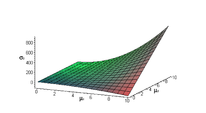
Figure 1: The Statistical Submanifold Evolution Surface

5 About the Stability of Geodesics on $\mathcal{M}_{s}$

We briefly investigate the stability of the trajectories of the RED model considered on $\mathcal{M}_{s}$. It is known $\left[8\right]$ that the Riemannian curvature of a manifold is closely connected with the behavior of the geodesics on it. If the Riemannian curvature of a manifold is negative, geodesics (initially parallel) rapidly diverge from one another. For the sake of simplicity, we assume very special initial conditions: $\alpha=\alpha_{1}=\alpha_{2}\ll\frac{1}{4}$, $\frac{A_{2}}{8\alpha_{2}^{2}}\ll 1$; $A_{1}$ and $B_{2}$ are arbitrary. However, the conclusion we reach can be generalized to more arbitrary initial conditions. Recall that $\mathcal{M}_{s}$ is the space of probability distributions $p^{(tot)}\left(\vec{x}|\vec{\theta}\right)$ labeled by parameters $\mu_{1},$ $\mu_{2},\sigma_{2}$. These parameters are the coordinates for the point $p^{(tot)}$, and in these coordinates a volume element $dV_{\mathcal{M}_{s}}$ reads,

$$dV_{\mathcal{M}_{s}}=g^{\frac{1}{2}}\left(\vec{\theta}\right)d^{3}\vec{\theta}\equiv\sqrt{g}d\mu_{1}d\mu_{2}d\sigma_{2}$$ (23)

where $g=|\det\left(g_{ij}\right)|=\frac{2}{\mu_{1}^{2}\sigma_{2}^{4}}$. Hence, using $\left(23\right)$, the volume of an extended region $\Delta V_{\mathcal{M}_{s}}$ of $\mathcal{M}_{s}$ is,

$$\Delta V_{\mathcal{M}_{s}}\left(\tau;\alpha\right)=V_{\mathcal{M}_{s}}\left(\tau\right)-V_{\mathcal{M}_{s}}\left(0\right)=\mathop{\displaystyle\int}\limits_{\mu_{1}\left(0\right)}^{\mu_{1}\left(\tau\right)}\mathop{\displaystyle\int}\limits_{\mu_{2}\left(0\right)}^{\mu_{2}\left(\tau\right)}\mathop{\displaystyle\int}\limits_{\sigma_{2}\left(0\right)}^{\sigma_{2}\left(\tau\right)}\sqrt{g}d\mu_{1}d\mu_{2}d\sigma_{2}\text{.}$$ (24)

Finally, using $\left(21\right)$ in $\left(24\right)$, the temporal evolution of the volume $\Delta V_{\mathcal{M}_{s}}$ becomes,

$$\Delta V_{\mathcal{M}_{s}}\left(\tau;\alpha\right)=\frac{A_{2}\tau}{\sqrt{2}}e^{\alpha\tau}.$$ (25)

Equation $\left(25\right)$ shows that volumes $\Delta V_{\mathcal{M}_{s}}\left(\tau;\alpha\right)$ increase exponentially with $\tau$. Consider the one-parameter $\left(\alpha\right)$ family of statistical volume elements $\mathcal{F}_{V_{\mathcal{M}_{s}}}\left(\alpha\right)\equiv\left\{\Delta V_{\mathcal{M}_{s}}\left(\tau;\alpha\right)\right\}_{\alpha}$. Note that $\alpha\equiv\alpha_{1}=$ $-\left(\frac{1}{\mu_{1}}\frac{d\mu_{1}}{d\tau}\right)_{\tau=0}>0$. The stability of the geodesics of the RED model may be studied from the behavior of the ratio $\mathit{r}_{V_{\mathcal{M}_{s}}}$ of neighboring volumes $\Delta V_{\mathcal{M}_{s}}\left(\tau;\alpha+\delta\alpha\right)$ and $\Delta V_{\mathcal{M}_{s}}\left(\tau;\alpha\right)$,

$$\mathit{r}_{V_{\mathcal{M}_{s}}}\overset{\text{def}}{=}\frac{\Delta V_{\mathcal{M}_{s}}\left(\tau;\alpha+\delta\alpha\right)}{\Delta V_{\mathcal{M}_{s}}\left(\tau;\alpha\right)}\text{.}$$ (26)

Positive $\delta\alpha$ is considered. The quantity $\mathit{r}_{V_{\mathcal{M}_{s}}}$ describes the relative volume changes in $\tau$ for volume elements with parameters $\alpha$ and $\alpha+\delta\alpha$. Substituting $\left(25\right)$ in $\left(26\right)$, we obtain

$$\mathit{r}_{V_{\mathcal{M}_{s}}}=e^{\delta\alpha\cdot\tau}\text{.}$$ (27)

Equation $\left(27\right)$ shows that the relative volume change ratio diverges exponentially under small perturbations of the initial conditions. Another useful quantity that encodes relevant information about the stability of neighbouring volume elements might be the entropy-like quantity $S$ defined as,

$$S\overset{\text{def}}{=}\log V_{\mathcal{M}_{s}}$$ (28)

where $V_{\mathcal{M}_{s}}$ is the average statistical volume element defined as,

$$V_{\mathcal{M}_{s}}\equiv\left\langle\Delta V_{\mathcal{M}_{s}}\right\rangle_{\tau}\overset{\text{def}}{=}\frac{1}{\tau}\mathop{\displaystyle\int}\limits_{0}^{\tau}\Delta V_{\mathcal{M}_{s}}\left(\tau^{\prime};\alpha\right)d\tau^{\prime}\text{.}$$ (29)

Indeed, substituting $\left(25\right)$ in $\left(29\right)$, the asymptotic limit of $\left(28\right)$ becomes,

$$S\approx\alpha\tau\text{.}$$ (30)

Doesn’t equation $\left(30\right)$ resemble the Zurek-Paz chaos criterion $\left[9\text{, }10\right]$ of linear entropy increase under stochastic perturbations? This question and a detailed investigation of the instability of neighbouring geodesics on different curved statistical manifolds are addressed in $\left[12\right]$ by studying the temporal behaviour of the Jacobi field intensity $\left[11\right]$ on such manifolds.

Our considerations suggest that suitable RED models may be constructed to describe chaotic dynamical systems and, furthermore, that a more careful analysis may lead to the clarification of the role of curvature in inferent methods for physics $\left[12\text{, }13\right]$.

6 Final Remarks

A RED model is considered. The space of microstates is $2D$ while all information necessary to study the dynamical evolution of such a system is contained in a $3D$ space of macrostates $\mathcal{M}_{s}$. It was shown that $\mathcal{M}_{s}$ possess the geometry of a curved manifold of constant negative curvature $\left(R=-1\right)$. The geodesics of the RED model are hyperbolic curves on the submanifold $\mathit{m}_{s}$ of $\mathcal{M}_{s}$. Furthermore, considerations of statistical volume elements suggest that these entropic dynamical models might be useful to mimic exponentially unstable systems. Provided the correct variables describing the true degrees of freedom of a system be identified, ED may lead to insights into the foundations of models of physics.

Acknowledgements: The authors are grateful to Prof. Ariel Caticha for very useful comments.

References

• (1) A. Caticha, ”Entropic Dynamics”, Bayesian Inference and Maximum Entropy Methods in Science and Engineering, ed. by R.L. Fry, AIP Conf. Proc. 617, 302 (2002).
• (2) A. Caticha, ”Relative Entropy and Inductive Inference”, Bayesian Inference and Maximum Entropy Methods in Science and Engineering,ed. by G. Erickson and Y. Zhai, AIP Conf. Proc. 707, 75 (2004).
• (3) A. Caticha and A. Giffin, ”Updating Probabilities”, presented at MaxEnt 2006, the 26th International Workshop on Bayesian Inference and Maximum Entropy Methods (Paris, France), arXiv:physics/0608185; A. Caticha, ”Maximum entropy and Bayesian data analysis: Entropic prior distributions”, Physical Review E 70, 046127 (2004).
• (4) S. Amari and H. Nagaoka, Methods of Information Geometry, American Mathematical Society, Oxford University Press, 2000.
• (5) C. Cafaro, S. A. Ali, A. Giffin, ”Irreversibility and Reversibility in Entropic Dynamical Models”, paper in preparation.
• (6) R.A. Fisher, ”Theory of statistical estimation” Proc. Cambridge Philos. Soc. 122, 700 (1925).
• (7) C.R. Rao, ”Information and accuracy attainable in the estimation of statistical parameters”, Bull. Calcutta Math. Soc. 37, 81 (1945).
• (8) V.I. Arnold, Mathematical Methods of Classical Physics, Springer-Verlag, 1989.
• (9) W. H. Zurek and J. P. Paz, ”Decoherence, Chaos, and the Second Law”, Phys. Rev. Lett. 72, 2508 (1994).
• (10) C. M. Caves and R. Schack, ”Unpredictability, Information, and Chaos”, Complexity 3, 46-57 (1997).
• (11) F. De Felice and C. J. S. Clarke, Relativity on Curved Manifolds, Cambridge University Press (1990).
• (12) C. Cafaro, S. A. Ali, ”Entropic Dynamical Randomness on Curved Statistical Manifolds”, paper in preparation.
• (13) B. Efron, ”Defining the curvature of a statistical problem”, Annals of Statistics 3, 1189 (1975).