Waiting time analysis of foreign currency exchange rates: Beyond the renewal-reward theorem

Abstract

We evaluate the average waiting time between observing the price of financial markets and the next price change, especially in an on-line foreign exchange trading service for individual customers via the internet. Basic technical idea of our present work is dependent on the so-called renewal-reward theorem. Assuming that stochastic processes of the market price changes could be regarded as a renewal process, we use the theorem to calculate the average waiting time of the process. In the conventional derivation of the theorem, it is apparently hard to evaluate the higher order moments of the waiting time. To overcome this type of difficulties, we attempt to derive the waiting time distribution $\Omega(s)$ directly for arbitrary time interval distribution (first passage time distribution) of the stochastic process $P_{W}(\tau)$ and observation time distribution $P_{O}(t)$ of customers. Our analysis enables us to evaluate not only the first moment (the average waiting time) but also any order of the higher moments of the waiting time. Moreover, in our formalism, it is possible to model the observation of the price on the internet by the customers in terms of the observation time distribution $P_{O}(t)$. We apply our analysis to the stochastic process of the on-line foreign exchange rate for individual customers from the Sony bank and compare the moments with the empirical data analysis.

I Introduction

Fluctuation has an important role in lots of phenomena appearing in our real world. For instance, a kind of magnetic alloy possesses magnetism in low temperature, whereas in high temperature, it losses the magnetism due to thermal fluctuation acting on each spin (a tiny magnet in atomic scale length). Thus, the large system undergoes a phase transition at some critical temperature and the transition occurs due to cooperative behavior of huge number of spins, to put it other way, due to competition between thermal fluctuation and exchange interaction between spin pairs making them point to the same direction [1].

To understand these kinds of macroscopic properties or collective behavior of the system from the microscopic point of view, statistical mechanics provides a good tool. Actually, statistical mechanics has been applied to various research subjects in which fluctuation is an essential key point, such as information processing [2] or economics including financial markets and game theory [3]. Especially, application of statistical-mechanical tools to economics, data analysis of financial markets — what we call econophysics — is one of the most developing research fields [4, 5, 6]. Financial data have attracted a lot of attentions of physicists as informative materials to investigate the macroscopic behavior of the markets from the microscopic statistical properties [4, 5, 6]. Some of these studies are restricted to the stochastic variables of the price changes (returns) and most of them is specified by a key word, that is to say, fat tails of the distributions [4]. However, the distribution of time intervals also might have important information about the markets and it is worth while for us to investigate these properties extensively [7, 8, 9, 10, 11, 12].

Such kinds of fluctuation in time intervals between events are not special phenomena in price changes in financial markets but very common in science. In fact, it is well-known that spike train of a single neuron in real brain is time series in which the difference between successive two spikes is not constant but fluctuated. This stochastic process specified by the so-called Inter-Spike Intervals (ISI) is one of such examples [13, 14]. The average of the ISI is about a few milli-second and the distribution of the intervals is well-described by the Gamma distribution [14].

On the other hand, in financial markets, for instance, the time intervals of two consecutive transactions of BUND futures (BUND is the German word for bond) and BTP futures (BTP is the middle and long term Italian Government bonds with fixed interest rates) traded at LIFFE (LIFFE stands for London International Financial Futures and Options Exchange) are $\sim 10$ seconds and are well-fitted by the so-called Mittag-Leffler function [8, 9, 10]. The Mittag-Leffler function behaves as a stretched exponential distribution for short time interval regime, whereas for the long time interval regime, the function has a power-law tails. Thus, the behavior of the distribution described by the Mittag-Leffler function is changed from the stretched exponential to the power-law at some critical point [15]. However, it is non-trivial to confirm if the Mittag-Leffler function supports any other kind of market data, for example, the market data filtered by some rate window.

As such market data, the Sony bank USD/JPY exchange rate [16], which is the rate for individual customers of the Sony bank in their on-line foreign exchange trading service, is a good example to be checked by the Mittag-Leffler function. Actually, our preliminary results imply that the Mittag-Leffler function does not support the Sony bank rate [17]. The Sony bank rate has $\sim 20$ minutes [18] as the average time interval which is extremely longer than the other market rate as the BUND future. This is because the Sony back rate can be regarded as the so-called first passage process [19, 20, 21, 22, 23, 24] of the raw market data.

TABLE I: Typical three examples with fluctuation between the events.

	ISI	BUND future	Sony bank rate
Average time interval	$\sim 3$ [ms]	$\sim 10$ [s]	$\sim 20$ [min]
PDF	Gamma	Mittag-Leffler	Weibull

In Table I, we list the average time intervals and the probability distribution function (PDF) that describes the data with fluctuation between the events for typical three examples, namely, the ISI, the BUND future and the Sony bank rate. From this table, an important question might be arisen. Namely, how long do the customers of the Sony bank should wait between observing the price and the next price change? This type of question is never occurred in the case of the ISI or the BUND future because the average time intervals are too short to evaluate such informative measure.

Obviously, for the customers, an important (relevant) quantity is sometimes a waiting time rather than a time interval between the rate changes. The waiting time we mentioned here is defined by the time for the customers to wait until the next price change since they try to observe it on the World Wide Web for example [16]. If the sequence of the time intervals has some correlations and the customers observe the rate at random on the time axis, the distribution of the waiting time is no longer identical to the distribution of the time intervals. In the previous studies [25, 26, 27], we assumed that the time intervals of the Sony bank USD/JPY exchange rates might follow a Weibull distribution and evaluated the average waiting time by means of the renewal-reward theorem [28, 29]. However, the conventional renewal-reward theorem is restricted to the case in which the customers observe the rate at random on the time axis and it is hard to extend the theorem to the situation in which the time for the customers to observe the rates obeys some arbitrary distributions.

To make these problems and difficulties clear, in this paper, we introduce a different way from the renewal-reward theorem to evaluate the higher-order moments of the waiting time for arbitrary time interval distribution of the price changes and observation time distribution by directly deriving the waiting time distribution. We first show that the result of the renewal-reward theorem [27] is recovered from our new formalism. Then, it becomes clear that our formulation is more general than the conventional renewal-reward theorem. As an advantage of our approach over the renewal-reward theorem, we can evaluate the higher-order moments of the waiting time, and moreover, it becomes possible to consider various situations in which the customers observe the rate according to arbitrary distribution of time.

This paper is organized as follows. In the next section II, we introduce the Sony bank rate [16] which is generated from the high-frequency foreign exchange market rate via the rate window with width $2\epsilon$ yen ($\epsilon=0.1$ yen for the Sony bank). In section III, we summarize a series of our previous studies related to the present paper. To understand the mechanism of the Sony bank rates as the first passage process [19, 20] of the raw market rate, in section IV, we carry out the computer simulations by making use of the GARCH (Generalized AutoRegressive Conditional Heteroscedasicity) model [30, 31, 32] with discrete returns as the time series behind the Sony bank rates. The effect of the rate window on the currency exchange rates is revealed. In the next section V, we explain our method to derive the waiting time distributions. We show that our treatment reproduces the result by the renewal-reward theorem. We also evaluate the deviation around the average waiting time for the Weibull first passage time distribution and uniform observation time distribution. We find that the resultant standard deviation is the same order as the average waiting time. We test our analysis for several cases of the observation time distributions and calculate the higher-order moments. The last section VI is concluding remarks.

II The Sony bank rates as a first passage process

The Sony bank rate (see Fig. 1) we shall deal with in this paper is the rate for individual customers of the Sony bank [16] in their on-line foreign exchange trading service via the internet.

Figure 1: Behavior of the Sony bank rates.

If the USD/JPY market rate changes by greater or equal to $0.1$ yen, the Sony bank USD/JPY exchange rate is updated to the market rate. In this sense, the Sony bank rate can be regarded as a kind of first passage processes [19, 20, 21, 22, 23, 24]. In Fig. 2, we show the mechanism of generating the Sony bank rate from the market rate (This process is sometimes refereed to as first exit process [33]). As shown in the figure, the difference between successive two points in the Sony bank rate becomes longer than the time intervals of the market rates.

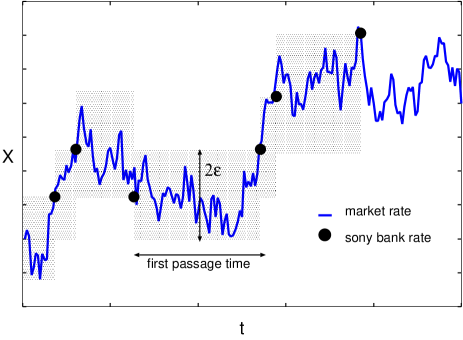
Figure 2: An illustration of generating the filtered rate (black circle) by the rate window with width $2\epsilon$ (shaded area) from the market rate (solid line).

In Table II, we show several data concerning the Sony bank USD/JPY rate vs. tick-by-tick data by Bloomberg for USD/JPY rate.

TABLE II: The Sony bank USD/JPY exchange rate vs. tick-by-tick data for USD/JPY exchange rate.

	Sony bank rate	tick-by-tick data
$\#$ of data a day	$\sim 70$	$\sim 10,000$
The smallest price change	$0.1$ yen	$0.01$ yen
Average interval between data	$\sim 20$ minutes	$\sim 7$ seconds

It is non-trivial problem to ask what kind of distribution is suitable to explain the distribution of the first passage time. For this problem, we attempted to check several statistics from both analytical and empirical points of view under the assumption that the first passage time might obey a non-exponential Weibull distribution [25, 26, 27]. We found that the data is well explained by a Weibull distribution. This fact means that the difference between successive Sony bank rate changes is fluctuated and has some memories.

III Previous related results

Before we start to explain what we attempt to do in the present paper, we shortly summarize the related results which were already obtained by the present authors.

• Sazuka (2006): We checked that the Sony bank rate is well-described by a Weibull distribution by some empirical data analysis (Weibull paper analysis, evaluation of Kullback-Leibuler, Hellinger divergence measures) [25, 26].

• Inoue and Sazuka (2006): We showed analytically that the crossover between non-Gaussian L$\acute{\rm e}$vy regime to Gaussian regime is observed even in the first passage process (which is the same process of the Sony bank rates) for a truncated L$\acute{\rm e}$vy flight (the so-called KoBoL process [34, 35, 36] in mathematics or mathematical finance) [37].

• Inoue and Sazuka (2006): We introduced queueing theoretical approach into the analysis of the Sony bank rate and evaluated average waiting time including expected returns. We also carried out computer simulations by using the GARCH model to investigate the effect of the rate window of the Sony bank [27].

• Sazuka (2006): We observed a phase transition between a Weibull distribution to a power-law distribution at some critical time from the empirical data analysis of the Sony bank rate [26].

• Sazuka and Inoue (2007): We introduced the Gini index to evaluate to what extent a Weibull distribution is well-fitted to explain the behavior of the first passage process of the Sony bank rate. The analytical evaluation and the empirical data analysis gave quite similar results [38, 17].

Then, we focus on the following two points.

• The effect of discreteness of returns in computer simulation by means of the GARCH model.

• Generalization of the renewal-reward theorem to calculate the higher order moments of the average waiting time or to evaluate the average waiting time for the case in which the observation time distribution of the trader is explicitly given.

This paper is intended as an investigation of these two points.

IV Computer simulations by the GARCH model with discrete returns

In the previous studies [27], we carried out computer simulations of the Sony bank USD/JPY exchange rates by assuming that the raw market data might be well-described by the GARCH model [30, 31, 32] in which the successive time intervals $\Delta t$ obey a Weibull distribution specified by a single parameter $m_{0}$, namely,

$$P(\Delta t) = \frac{m_{0}\,(\Delta t)^{m_{0}-1}}{a}\,{\exp}\left[-\frac{(\Delta t)^{m_{0}}}{a}\right].$$ (1)

In [27], we set $a=1$ for a scaling parameter for simplicity to handle. We investigated the stochastic process generated by the rate window and estimated the distribution of time intervals of the stochastic process filtered by the rate window. Then, we assumed that the output of the filter having rate window with width $2\epsilon$ also follows a Weibull distribution with $m(\neq m_{0})$ and estimated $m$ by means of Weibull paper analysis. The plot $m$-$m_{0}$ was obtained and the effect of the rate window on the market rate became clear. However, in those simulations, we assumed that the smallest price change (return) might take continuous values for simplicity to carry out the simulations. As we see in Table 1, the smallest price change unit of the tick-by-tick market data is $0.01$ yen. Therefore, we should modify our computer simulations of the GARCH model by taking into account the discreteness of the price change. In this section, we show the result of the computer simulations. To this end, we deal with here the following modified GARCH(1,1) model [27]:

$$X_{t} = X_{t-\Delta t}+{\mathcal{N}}(0,\sigma_{t}^{2})$$ (2)

$$\sigma_{t}^{2} = \alpha_{0}+\alpha_{1}X_{t-\Delta t}^{2}+\beta_{1}\sigma_{t-\Delta t}^{2}$$ (3)

where the time interval $\Delta t$ obeys a Weibull distribution with parameters $(m,a)$, namely,

$$P(\Delta t) = \frac{m(\Delta t)^{m-1}}{a}\,{\exp}\left[-\frac{(\Delta t)^{m}}{a}\right]$$ (4)

and ${\mathcal{N}}(0,\sigma_{t}^{2})$ in this expression stands for a Gaussian with zero-mean and time dependent variance $\sigma_{t}^{2}$. For simplicity, we set the parameter $a$ as $a=1$. We should notice that the GARCH(1,1) model has the variance $\sigma^{2}$ after observing on a long time intervals $t\to\infty$ and $\sigma^{2}$ leads to

$$\sigma^{2} = \frac{\alpha_{0}}{1-\alpha_{1}-\beta_{1}}.$$ (5)

To make the return $X_{t}$ discrete, for each time step, we regenerate $X_{t}$ by using the next map:

$$X_{t} = \Psi_{\Delta}(X_{t})\equiv\Delta\,{\rm ceil}(\Delta^{-1}X_{t})$$ (6)

where the function ${\rm ceil}(x)$ is defined as the smallest integer no less than $x$. The parameter $\Delta$ appearing in (6) means the length of the minimal variation of the return.

Figure 3: The pdf of the GARCH(1,1) model with discrete returns. We set $\Delta=0.1$ (upper panel) and $\Delta=0.2$ (lower panel). The inset is behavior around small $Y$ regime.

In Fig. 3, we plot the pdf of $Y_{t}=X_{t}-X_{t-\Delta t}$ for the above discrete GARCH model with a parameter set: $(\alpha_{0},\alpha_{1},\beta_{1})=(0.4,0.3,0.3)$ which gives the kurtosis $\kappa=4.17$ and variance $\sigma^{2}=1$ in the limit of $t\to\infty$, and $\Delta=0.1$ and $\epsilon=\sigma=1$. We should keep in mind that the ratio between the width of the rate window and the minimal change of the rate, namely, $\epsilon/\Delta=10$ is the same as that of the Sony bank rate. From this figure, we recognize that the return $Y$ actually takes discrete values as expected.

To investigate the effect of the rate window with width $2\epsilon$, we estimate the Weibull parameter $m$ of the output sequence from the rate window by means of the so-called Weibull paper analysis [25, 26, 27] for the cumulative Weibull distribution.

Figure 4: The Weibull paper for the case of $m_{0}=0.6$ (upper panel) and $1.2$ (lower panel). We choose $\Delta=0.1$.

From Fig. 4, we find that for the case of $m_{0}=0.6,1.2$, the first passage time distribution also obeys a Weibull distribution with a parameter $m$ which is different from $m_{0}$.

Figure 5: The relation between $m_{0}$ and $m$ for the case of $\Delta=0,0.1,0.2$ and $0.5$. For each $\Delta$, we carried out $10$ independent runs of simulations.

In Fig. 5, we plot the relation between $m_{0}$ and $m$ for several values of $\Delta$. From this figure, we find that the relation for the discrete cases with $\Delta=0.1$ and $0.2$ are almost same as the relation for the continuous case $\Delta=0$ reported in our previous papers [27]. Meaningful differences are observed if we increase the value of $\Delta$ up to $0.5$. This result provides us a justification of our previous GARCH modeling [27] of the market rate to simulate the Sony bank USD/JPY exchange rates on the assumption that the minimum price change could take infinitesimal values.

V Derivation of the waiting time distribution

In the previous studies [27], we evaluated the average waiting time for the customers to wait by the next price change since they attempt to observe the price by making use of the renewal-reward theorem [28, 29]. However, the theorem itself is obviously restricted to deriving only the first moment of the waiting time. From this reason, it is very hard to evaluate, for instance, the standard deviation from the average waiting time within the framework of the theorem (for example, see the proof of the theorem provided in [29]). Thus, we need another procedure to calculate it without the conventional derivation of the renewal-reward theorem. In this section, we directly derive the distribution of the waiting time. Our approach here enables us to evaluate not only the first moment of the waiting time but also any order of the moment. This section is a core part of this paper.

V-A The probability distribution of the waiting time

We first derive the probability distribution function of the waiting time $s$. Then, let us suppose that the difference between successive two points of the Sony bank rate change, namely, the first passage time $\tau$ follows $P_{W}(\tau)$. Then, the customers observe the rate in time $t$ ($0\leq t\leq\tau$) that should be measured from the point at which the rate changes previously. In Fig. 6, we show the relation among these points $\tau,t$ and $s$ in time axis.

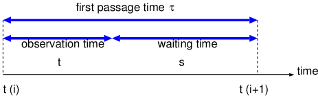
Figure 6: The relation these points $\tau,t$ and $s$ in time axis. The first passage time $\tau$ is given by $\tau=t(i+1)-t(i)$. The observation time is measured from the point $t(i)$.

The waiting time of the customers is naturally defined by $s\equiv\tau-t$. We should notice that the distribution $\Omega(s)$ is written in terms of the first passage time distribution $P_{W}(\tau)$ and the observation time distribution $P_{O}$(t) of the customers as

$$\Omega(s) \propto \int_{0}^{\infty}d\tau\int_{0}^{\tau}dt\,Q(s|\tau,t)P_{O}(t)P_{W}(\tau).$$ (7)

Obviously, probability $Q(s|\tau,t)$ that the waiting time takes $s$ provided that the observation time and the first passage time are given as $t$ and $\tau$, respectively, is given as

$$Q(s|\tau,t) = \delta(s-\tau+t)$$ (8)

with the delta function $\delta(x)$. Taking into account the normalization constant of $\Omega(s)$, we have

$$\Omega(s)=\frac{\int_{0}^{\infty}d\tau P_{W}(\tau)\int_{0}^{\tau}dt\,\delta(s-\tau+t)P_{O}(t)}{\int_{0}^{\infty}ds\int_{0}^{\infty}d\tau P_{W}(\tau)\int_{0}^{\tau}dt\,\delta(s-\tau+t)P_{O}(t)}$$ (9)

where $t$ denotes the observation time for the customers. We should notice that the result of the renewal-reward theorem : $w=\langle s\rangle=E(\tau^{2})/2E(\tau)$ (see for example [29]) is recovered by inserting the uniform observation time distribution $P_{O}(t)=1$ into the above expression as

$$w = \langle s\rangle=\int_{0}^{\infty}dss\Omega(s)=\frac{\int_{0}^{\infty}dss\int_{s}^{\infty}d\tau P_{W}(\tau)}{\int_{0}^{\infty}ds\int_{s}^{\infty}d\tau P_{W}(\tau)}$$ (10)

$$= \frac{\int_{0}^{\infty}\frac{d}{dt}\{s^{2}/2\}ds\int_{s}^{\infty}d\tau P_{W}(\tau)}{\int_{0}^{\infty}\frac{d}{ds}\{s\}ds\int_{s}^{\infty}d\tau P_{W}(\tau)}$$

$$= \frac{(1/2)\int_{0}^{\infty}s^{2}P_{W}(s)ds}{\int_{0}^{\infty}sP_{W}(s)ds}=\frac{E(\tau^{2})}{2E(\tau)}$$

where we defined the $n$-th moment of the first passage time $E(\tau^{n})$ by

$$E(\tau^{n}) = \int_{0}^{\infty}dss^{n}P_{W}(s).$$ (11)

More generally, we may set $P_{O}(t)$. For this general form of the observation time distribution, the probability distribution of the waiting time $s$ is given as follows.

$$\Omega(s) = \frac{\int_{s}^{\infty}d\tau P_{W}(\tau)P_{O}(\tau-s)}{\int_{0}^{\infty}ds\int_{s}^{\infty}d\tau P_{W}(\tau)P_{O}(\tau-s)}$$ (12)

$$= \frac{\int_{s}^{\infty}d\tau P_{W}(\tau)P_{O}(\tau-s)}{E(t)-\delta_{1}}$$

where we defined $\delta_{n}$ by

$$\delta_{n} = \int_{0}^{\infty}\frac{dss^{n}}{n}\int_{s}^{\infty}P_{W}(\tau)\frac{\partial P_{O}(\tau-s)}{\partial s}.$$ (13)

By using the same way as the derivation of the distribution $\Omega(s)$, we easily obtained the first two moments of the waiting time distribution as

$$\langle s\rangle = \frac{E(\tau^{2})/2-\delta_{2}}{E(\tau)-\delta_{1}},\,\,\,\langle s^{2}\rangle=\frac{E(\tau^{3})/3-\delta_{3}}{E(\tau)-\delta_{1}}$$ (14)

and the standard deviation leads to

$$\sigma=\sqrt{\frac{\{4E(\tau^{3})E(\tau)-3E(\tau^{2})\}+G_{\delta_{1},\delta_{2},\delta_{3}}}{12(E(\tau)-\delta_{1})^{2}}}$$ (15)

$$G_{\delta_{1},\delta_{2},\delta_{3}} = -4\delta_{1}E(\tau^{3})-12\delta_{3}E(\tau)$$ (16)

$$+ 12\delta_{2}E(\tau^{2})+12\delta_{1}\delta_{3}-12\delta_{2}^{2}$$

where we defined

$$\langle s^{n}\rangle = \int_{0}^{\infty}dss^{n}\Omega(s).$$ (17)

Thus, this probability distribution $\Omega(s)$ enables us to evaluate any order of the moments for the waiting time.

In following, we evaluate the average waiting time and the deviation around the average for typical two cases, namely, $P_{O}(t)=1$ and $P_{O}(t)={\rm e}^{-t/\tau_{0}}$.

V-A1 The customers’ observation follows $P_{O}(t)=1$

We first consider the case of $P_{O}(\tau)=1$. This case corresponds to the result obtained by the renewal-reward theorem [27]. Obviously, we find that $\delta_{n}=0$ holds for arbitrary integer $n$. Thus, the waiting time distribution $\Omega(s)$ leads to

$$\Omega(s) = \frac{\int_{s}^{\infty}P_{W}(\tau)}{E(\tau)}.$$ (18)

Then, the average waiting time and the deviation around the value lead to

$$w = \frac{E(\tau^{2})}{2E(\tau)},\,\,\,\,\sigma=\sqrt{\frac{4E(\tau^{3})E(\tau)-3E(\tau^{2})^{2}}{12E(\tau)^{2}}}.$$ (19)

For a Weibull distribution having the parameters $m,a$, the above results are rewritten by

$$\Omega(s) = \frac{m\,{\rm e}^{-s^{m}/a}}{a^{1/m}\Gamma\left(\frac{1}{m}\right)}$$ (20)

$$w = a^{1/m}\frac{\Gamma\left(\frac{2}{m}\right)}{\Gamma\left(\frac{1}{m}\right)}$$ (21)

$$\sigma = \frac{a^{1/m}\sqrt{\Gamma(1/m)\Gamma(3/m)-\Gamma(2/m)^{2}}}{\Gamma(1/m)}$$ (22)

where we defined the Gamma function as

$$\Gamma(x) = \int_{0}^{\infty}dt\,t^{x-1}{\rm e}^{-t}.$$ (23)

It is important for us to notice that for an exponential distribution $m=1$, we have $w=\sigma=a$ by taking into account the fact that $\Gamma(n)=(n-1)!$. Moreover, the average waiting time $w$ is identical to the average time interval $E(\tau)$ since $w=E(\tau^{2})/2E(\tau)=E(\tau)$ holds if and only if $m=1$ (The rate changes follow a Poisson arrival process). These results are already obtained in our previous studies [27]. In Fig. 7, we plot the distribution $\Omega(s)$ and the standard deviation $\sigma$ for a Weibull distribution. Especially, for the Sony bank case $a=49.6345,m=0.585$, we find $\sigma=60.2284$ minutes.

Figure 7: The distribution of waiting time for a Weibull distributing $\Omega(s)$ with $a=1$ and $m=0.59,1$ and $2$ (upper panel). In the lower panel, we plot the standard deviation $\sigma$ for a Weibull distribution with $a=49.6345$ as a function of $m$.

V-A2 The customers’ observation follows $P_{O}(t)={\rm e}^{-t/\tau_{0}}$

We test the other observation time distribution of the customers. For instance, we might choose $P_{O}(t)={\rm e}^{-t/\tau_{0}}$ on the assumption that the customers might observe the rate more frequently within the time scale $\tau_{0}$ around the previous rate change than the time scale longer than $\tau_{0}$. Such a case could be possible if the system provides some redundant information about the point of the rate change to customers as quickly as possible.

For this choice of the observation time distribution $P_{O}(t)={\rm e}^{-t/\tau_{0}}$, we have

$$\delta_{n} = \frac{1}{\tau_{0}}\int_{0}^{\infty}\frac{dss^{n}\,{\rm e}^{s/\tau_{0}}}{n}\int_{s}^{\infty}d\tau P_{W}(\tau)\,{\rm e}^{-\tau/\tau_{0}}.$$ (24)

Therefore, from equations (12),(14) and (15), it is possible for us to derive the waiting time distribution $\Omega(s)$ and average waiting time and the deviation from the value. For the choice of a Weibull first passage time distribution $P_{W}(\tau)$, we need some algebra, but easily obtain

$$\Omega(s) = \frac{{\rm e}^{s/\tau_{0}}\mu_{a}^{m}(\tau_{0};s)}{\frac{a^{1/m}}{m}\Gamma\left(\frac{1}{m}\right)-\frac{1}{\tau_{0}}\int_{0}^{\infty}sds\,\mu_{a}^{m}(\tau_{0};s)}$$ (25)

where we defined $\mu_{a}^{m}(\tau_{0};s)$ by the following integral form:

$$\mu_{a}^{m}(\tau_{0};s) = \int_{a^{-1}s^{m}}^{\infty}dz\,{\exp}\left[-z-\frac{(az)^{1/m}}{\tau_{0}}\right].$$ (26)

In Fig. 8, we plot the distribution for the case of several values of $\tau_{0}$ and $m=0.585$ and $a=49.6345$.

Figure 8: The waiting time distribution $\Omega(s)$ for the case of the weight function $P_{O}(t)={\rm e}^{-t/\tau_{0}}$ with several values of $\tau_{0}$. For each plot, we set $m=0.585$ and $a=49.6345$.

From this figure, we find that the probability for large waiting time $s$ increases as the relaxation time $\tau_{0}$ increases. We should notice that the case of $\tau_{0}\to\infty$ turns out to be random observation by the customers.

From the equations (14), the first two moments are obtained by

$$w = \langle s\rangle=\frac{\frac{a^{2/m}}{m}\Gamma\left(\frac{2}{m}\right)-\tau_{0}^{-1}\xi_{m,a}^{(2)}(\tau_{0})}{\frac{a^{1/m}}{m}\Gamma\left(\frac{1}{m}\right)-\tau_{0}^{-1}\xi_{m,a}^{(1)}(\tau_{0})}$$ (27)

$$\langle s^{2}\rangle = \frac{\frac{a^{3/m}}{m}\Gamma\left(\frac{3}{m}\right)-\tau_{0}^{-1}\xi_{m,a}^{(3)}(\tau_{0})}{\frac{a^{1/m}}{m}\Gamma\left(\frac{1}{m}\right)-\tau_{0}^{-1}\xi_{m,a}^{(1)}(\tau_{0})}$$ (28)

where we defined

$$\xi_{m,a}^{(n)}(\tau_{0}) = \int_{0}^{\infty}\frac{dss^{n}{\rm e}^{s/\tau_{0}}}{n}\mu_{a}^{m}(\tau_{0};s).$$ (29)

It should be noted that for large $\tau_{0}$, the leading order of the function $\xi_{m,a}^{(n)}(\tau)$ is evaluated as $\xi_{m,a}^{(n)}(\tau)=1+{\mathcal{O}}(\tau_{0}^{-1})$. Thus, the average waiting time $w$ for $P_{O}(t)={\rm e}^{-t/\tau_{0}}$ becomes smaller than that obtained for $P_{O}(t)=1$ as

$$w = a^{1/m}\frac{\Gamma\left(\frac{2}{m}\right)}{\Gamma\left(\frac{1}{m}\right)}-{\mathcal{O}}(\tau_{0}^{-1}).$$ (30)

However, at the same time, the standard deviation also behaves as

$$\sigma=\frac{a^{1/m}\sqrt{\Gamma(1/m)\Gamma(3/m)-\Gamma(2/m)^{2}}}{\Gamma(1/m)}-{\mathcal{O}}(\tau_{0}^{-1}).$$ (31)

This means that even if the trader observe the rate according to a priori knowledge, namely, the observation time distribution $P_{O}(t)={\rm e}^{-t/\tau_{0}}$, the standard deviation from the average waiting time is the same order as the average waiting time itself.

In this paper, we considered just only two cases of the observation time distribution $P_{O}(t)$, however, the choice of the distribution is completely arbitrary. The detail and more carefully analysis of this point will be reported in our forth coming article [17].

V-A3 Comparison with empirical data analysis

It is time for us to compare the analytical result with that of the empirical data analysis. For uniform observation time distribution $P_{O}(t)=1$, we obtained $\sigma=60.2284$ minutes. On the other hand, from empirical data analysis, we evaluate the quantity (19) by sampling the moment as $E(\tau^{n})=(1/N)\sum_{i=1}^{N}\tau_{i}^{n}$ directly from Sony bank rate data [16] and find $\sigma=74.3464$ minutes. There exists a finite gap between the theoretical prediction and the result by the empirical data analysis, however, the both are the same order. The gap might become small if we take into account the power-law tail of the first passage time distribution. In fact, our preliminary investigation shows that for the average waiting time, the power-law tail makes the gap between the theoretical prediction and empirical observation small [17]. Therefore, the same tail-effect is reasonably expected even in the analysis of the deviation.

VI Concluding remarks

In this paper, we proposed a different procedure from the conventional derivation of the renewal-reward theorem. This derivation enables us to evaluate arbitrary order of the moments of the waiting time of the on-line foreign exchange trading rate for the individual customers. We directly derived the waiting time distribution and evaluated the deviation around the average waiting time, which is not supported by the renewal-reward theorem, for the Sony bank USD/JPY exchange rates. We tested our analysis for several cases of the observation time distribution of the customers and found that the average waiting time and deviation from the value are the same order even if the customers possesses a priori knowledge as a form of the observation time distribution as $P_{O}(t)={\rm e}^{-t/\tau_{0}}$. This result might be understood as follows. As we mentioned, the system we dealt with in this paper has two types of fluctuations, namely, fluctuation in the intervals of events (price changes) and fluctuation in the observation time for the individual customers to observe the rate through the World Wide Web. As well-known, in the $N$-body systems ($N$ is extremely large), there exists theremal fluctuation (quantum-mechanical fluctuation as well in low temperature) affecting on each particle, however, the macroscopic variables (the averages over the Gibbs distribution) like pressure or internal energy are determined as of order $1$ objects and the deviation from the average becomes zero as $N^{-1/2}$. This is a reason why statistical mechanics could predict a lot of physical quantities and we could compare the prediction with the same quantity which was observed in experiments. On the other hand, although the financial market price changes are taken place as a result of trading by many people, the observed rate itself is regarded as a result of effective single particle problems (a complicated single random walker) and there is no such scale parameter like the number of particle $N$. This is an intuitive account of the result, namely, the average and the deviation are the same order even if there exist two kinds of fluctuation in the systems.

Remaining problems concerning the analysis of the Sony bank rate are firstly to investigate the effect of the tail of the first passage time distribution. Our preliminary observation from the empirical data implied that, at some critical point, the distribution changes its shape from a Weibull-law to a power-law [26]. Therefore, it is important for us to check to what extent the prediction by the renewal-reward theorem is modified by taking into account the tail effect of the first passage time distribution. Secondly, we should show explicitly that the first passage time distribution described by the Mittag-Leffler function [9, 10, 15]:

$$P(\tau) = \sum_{n=0}^{\infty}(-1)^{n}\frac{(\tau/\tau_{0})^{\beta n}}{\Gamma(\beta n+1)}\,\,\,\,\,\,\,(0<\beta<1)$$ (32)

is impossible to realize the first passage process of the Sony bank by comparing the analytical result of the average waiting time or the Gini index with those obtained by the empirical data analysis. The detail of these studies will be reported shortly in [17].

As we showed in this paper, our queueing theoretical approach might be useful for us to build artificial markets such as the on-line trading service so as to have a suitable waiting time for the individual customers by controlling the width of the rate window. Moreover, theoretical framework we provided here could predict the average waiting time including the deviation.

We hope that our strategy in order to analyze the stochastic process of markets from the view point of the waiting time of the customers might help researchers or engineers when they attempt to construct a suitable system for their customers.

References

- [1] H.E. Stanley, Introduction to Phase Transitions and Critical Phenomena, Oxford University Press (1987).
- [2] H. Nishimori, Statistical Physics of Spin Glasses and Information Processing : An Introduction, Oxford University Press (2001).
- [3] A.C.C. Coolen, The Mathematical Theory Of Minority Games: Statistical Mechanics Of Interacting Agents (Oxford Finance), Oxford University Press, (2006).
- [4] R.N. Mantegna and H.E. Stanley, An Introduction to Econophysics : Correlations and Complexity in Finance, Cambridge University Press (2000).
- [5] J.-P. Bouchaud and M. Potters, Theory of Financial Risk and Derivative Pricing, Cambridge University Press (2000).
- [6] J. Voit, The Statistical Mechanics of Financial Markets, Springer (2001).
- [7] R. F. Engle and J. R. Russel, Econometrica 66, 1127 (1998).
- [8] F. Mainardi, M. Raberto, R. Gorenflo and E. Scalas, Physica A 287, 468 (2000).
- [9] M. Raberto, E. Scalas and F. Mainardi, Physica A 314, 749 (2002).
- [10] E. Scalas, R. Gorenflo, H. Luckock, F. Mainardi, M. Mantelli and M. Raberto, Quantitative Finance 4, 695 (2004).
- [11] T. Kaizoji and M. Kaizoji, Physica A 336, 563 (2004).
- [12] E. Scalas, Physica A 362, 225 (2006).
- [13] H.C. Tuckwell, Stochastic Processes in the Neuroscience, Society for industrial and applied mathematics, Philadelphia, Pennsylvania (1989).
- [14] W. Gerstner and W. Kistler, Spiking Neuron Models, Cambridge University Press (2002).
- [15] R. Gorenflo and F. Mainardi, The asymptotic universality of the Mittag-Leffler waiting time law in continuous random walks, Lecture note at WE-Heraeus-Seminar on Physikzentrum Bad-Honnef (Germany), 12-16 July (2006).
- [16] http://moneykit.net
- [17] N. Sazuka and J. Inoue, in preparation.
- [18] N. Sazuka, Eur. Phys. J. B 50, 129 (2006).
- [19] S. Redner, A Guide to First-Passage Processes, Cambridge University Press (2001).
- [20] N.G. van Kappen, Stochastic Processes in Physics and Chemistry, North Holland, Amsterdam (1992).
- [21] C.W. Gardiner, Handbook of Stochastic Methods for Physics, Chemistry and Natural Sciences, Springer Berlin, (1983).
- [22] H. Risken, The Fokker-Plank Equation : Methods of Solution and Applications, Springer Berlin, (1984).
- [23] I. Simonsen, M.H. Jensen and A. Johansen, Eur. Phys. J. B 27, 583 (2002).
- [24] S. Kurihara, T. Mizuno, H. Takayasu and M. Takayasu, The Application of Econophysics, H. Takayasu (Ed.), pp. 169-173, Springer (2003).
- [25] N. Sazuka, Busseikenkyu 86 (in Japanese) (2006).
- [26] N. Sazuka, http://arxiv.org/abs/physics/0606005, to appear in Physica A.
- [27] J. Inoue and N. Sazuka, http://arxiv.org/abs/physics/0606040, submitted to Quantitative Finance.
- [28] H.C. Tijms, A first Course in Stochastic Models, John Wiley Sons (2003).
- [29] S. Oishi, Queueing Theory, CORONA PUBLISHING CO., LTD (in Japanese) (2003).
- [30] R.F. Engle, Econometrica 50, 987 (1982).
- [31] T. Ballerslev, Econometrics 31, 307 (1986).
- [32] J. Franke, W. Hrdle and C.M. Hafner, Statistics of Financial Markets : An Introduction, Springer (2004).
- [33] M. Montero and J. Masoliver, http://arxiv.org/abs/physics/0607268 (2006).
- [34] Lvy Processes in Finance: Pricing Financial Derivatives, Weley, New York (2003).
- [35] I. Koponen, Physical Review E 52, 1197 (1995).
- [36] S.I. Boyarchenko and S.Z. Levendorski, Generalizations of the Black-Scholes equation for truncated Lvy processes, Working paper (1999).
- [37] J. Inoue and N. Sazuka, http://arxiv.org/abs/physics/0606038, submitted to Physical Review E.
- [38] N. Sazuka and J. Inoue, http://arxiv.org/abs/physics/0701008, submitted to Physica A.