Betweenness Centrality of Fractal and Non-Fractal Scale-Free Model Networks and Tests on Real Networks

Abstract

We study the betweenness centrality of fractal and non-fractal scale-free network models as well as real networks. We show that the correlation between degree and betweenness centrality $C$ of nodes is much weaker in fractal network models compared to non-fractal models. We also show that nodes of both fractal and non-fractal scale-free networks have power law betweenness centrality distribution $P(C)\sim C^{-\delta}$. We find that for non-fractal scale-free networks $\delta=2$, and for fractal scale-free networks $\delta=2-1/d_{B}$, where $d_{B}$ is the dimension of the fractal network. We support these results by explicit calculations on four real networks: pharmaceutical firms ($N=6776$), yeast ($N=1458$), WWW ($N=2526$), and a sample of Internet network at AS level ($N=20566$), where $N$ is the number of nodes in the largest connected component of a network. We also study the crossover phenomenon from fractal to non-fractal networks upon adding random edges to a fractal network. We show that the crossover length $\ell^{*}$, separating fractal and non-fractal regimes, scales with dimension $d_{B}$ of the network as $p^{-1/d_{B}}$, where $p$ is the density of random edges added to the network. We find that the correlation between degree and betweenness centrality increases with $p$.

I Introduction

Studies of complex networks have recently attracted much attention in diverse areas of science Barabasi_rmp_review ; evol_of_nw ; evol_and_struct ; compl_nw . Many real-world complex systems can be usefully described in the language of networks or graphs, as sets of nodes connected by edges ER ; ER_random graphs . Although different in nature many networks are found to possess common properties. Many networks are known to have a “small-world” property collect_dynam ; sw_problem ; bollobas ; diam_of_www : despite their large size, the shortest path between any two nodes is very small. In addition, many real networks are scale-free (SF) Barabasi_rmp_review ; evol_of_nw ; evol_and_struct ; compl_nw ; faloutsos_etall ; scaling_in_nw , well approximated by a power-law tail in degree distribution, $P(k)\sim k^{-\lambda}$, where $k$ is the number of links per node.

Many networks, such as the WWW and biological networks have self-similar properties and are fractals repulsion ; self-sim ; skeleton_and_fractal ; crit_and_supercrit_skelet ; dissasort . The box-counting algorithm box_count ; self-sim allows to calculate their fractal dimensions $d_{B}$ from the box-counting relation

$$N_{B}\sim\ell_{B}^{-d_{B}},$$ (1)

where $N_{B}$ is the minimum number of boxes of size $\ell_{B}$ needed to cover the entire network (Appendix B). Structural analysis of fractal networks shows that the emergence of SF fractal networks is mainly due to disassortativity or repulsion between hubs repulsion . That is, nodes of large degree (hubs) tend to connect to nodes of small degree, giving life to the paradigm “the rich get richer but at the expense of the poor.” To incorporate this feature, a growth model of SF fractal networks that combines a renormalization growth approach with repulsion between hubs has been introduced repulsion . It has also been noted repulsion that the traditional measure of assortativity of networks, the Pearson coefficient $r$ assortativity does not distinguish between fractal and non-fractal network since it is not invariant under renormalization.

Here, we study properties of fractal and non-fractal networks, including both models and real networks. We focus on one important characteristic of networks, the betweenness centrality (C), centr_definition ; centr_book ; centr_handbook ; newman , defined as,

$$C(i)\equiv\sum_{j,k}\frac{\sigma_{j,k}(i)}{\sigma_{j,k}},$$ (2)

where $\sigma_{j,k}(i)$ is the number of shortest paths between nodes $j$ and $k$ that pass node $i$ and $\sigma_{j,k}$ is the total number of shortest paths between nodes $j$ and $k$.

The betweenness centrality of a node is proportional to the number of shortest paths that go through it. Since transport is more efficient along shortest paths, nodes of high betweenness centrality $C$ are important for transport. If they are blocked, transport becomes less efficient. On the other hand, if the capacitance of high $C$ nodes is improved, transport becomes significantly better superhighways .

Here we show that fractal networks possess much lower correlation between betweenness centrality and degree of a node compared to non-fractal networks. We find that in fractal networks even small degree nodes can have very large betweenness centrality while in non-fractal networks large betweenness centrality is mainly attributed to large degree nodes. We also show that the betweenness centrality distribution in SF fractal networks obeys a power law. We study the effect of adding random edges to fractal networks. We find that adding a small number of random edges to fractal networks significantly decreases the betweenness centrality of small degree nodes. However, adding random edges to non-fractal networks has a significantly smaller effect on the betweenness centrality.

We also analyze the transition from fractal to non-fractal networks by adding random edges and show both analytically and numerically that there exists a crossover length $\ell^{*}$ such that for length scales $\ell<\ell^{*}$ the topology of the network is fractal while for $\ell>\ell^{*}$ it is non-fractal. The crossover length scales as $\ell^{*}\sim p^{-1/d_{B}}$, where $p$ is the number of random edges per node. We analyze seven SF model networks and four real networks.

The four real networks we analyze are the network of pharmaceutical firms Pharm , an Internet network at the AS level obtained from the DIMES project dimes ; Shai , PIN network of yeast Barabasi ; yeast and WWW network of University of Western Sydney uws . Pharmaceutical network is the network of nodes representing firms in the worldwide pharmaceutical industry and the links are collaborative agreements among them. The Internet network represents a sample of the internet structure at the Autonomous Systems(AS) level. The Protein Interaction Network (PIN) of yeast represents proteins as nodes and interactions between them as links between nodes. The WWW network of University of Western Sydney represents web pages (nodes) targeted by links from the uws.edu.au domain. Basic properties of the considered networks are summarized in Table. I.

The manuscript is organized as follows: In section II, we study correlation between the betweenness centrality and degree of nodes, and we compare fractal and non-fractal networks. We analyze the betweenness centrality variance $\sigma_{C}(k)$ of nodes of the same degree $k$ and introduce a correlation coefficient $R$ that describes the strength of betweenness centrality degree correlation. We also analyze the betweenness centrality distribution $P(C)$ of several model and real networks. In section III we study the transition from fractal to non-fractal networks with randomly added edges. Appendix A provides a short summary of the fractal growth model introduced in repulsion . Appendix B discusses the box covering method and its approximations.

II Betweenness centrality of fractal and non-fractal networks

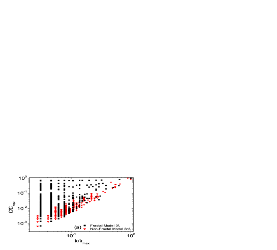
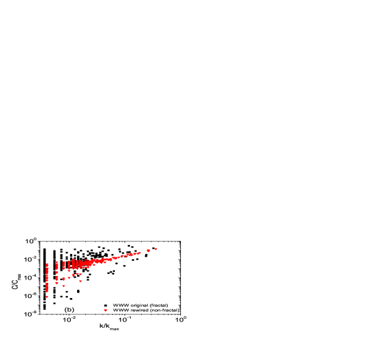
Figure 1: (a) Betweenness centrality versus degree correlation profiles of fractal and non-fractal network models. Note the broader range of betweenness centrality values of small degree nodes of fractal network compared to that of the non-fractal network. (b) Betweenness centrality versus degree correlation profiles of Uni Western Sydney WWW (fractal) network and its random counterpart. The randomly rewired network is non-fractal. Betweenness centrality and degree are correlated much stronger in nodes of the random rewired network.

It is generally accepted Attack_vulnerability that in many networks nodes having a larger degree also have a larger betweenness centrality. Indeed, the larger the degree of a node, the larger the chance that many of the shortest paths will pass through this node; the chance of many shortest paths passing a low degree node is presumably small. Here we show that this is not the case for fractal SF networks. As seen in Fig. 1(a) small degree nodes in fractal SF networks have a broad range of betweenness centrality values. The betweenness centrality of many small degree nodes can be comparable to that of the largest hubs of the network. For non-fractal networks, on the other hand, degree and betweenness centrality of nodes are strongly correlated.

To demonstrate the difference in the relation between degree and betweenness centrality in real networks we compare original networks with their random (uncorrelated) counterparts. We construct the random counterpart network by rewiring the edges of the original network, yet preserving the degrees of the nodes and enforcing its connectivity. As a result we obtain a random network with the same degree distribution which is always non-fractal regardless of the original network. As seen in Fig. 1(b),the betweenness centrality-degree correlation of a random network obtained by rewiring edges of the WWW network is much stronger compared to that of the original network. Ranges of betweenness centrality values for a given degree decrease significantly as we randomly rewire edges of a fractal SF network.

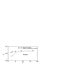
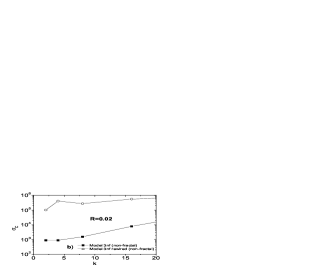
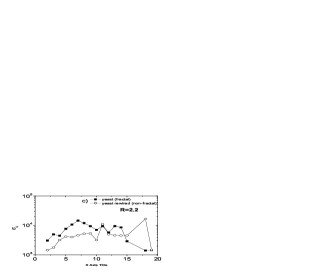
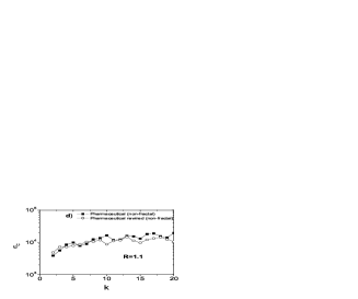
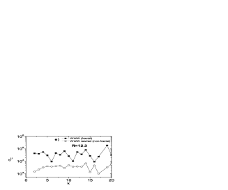
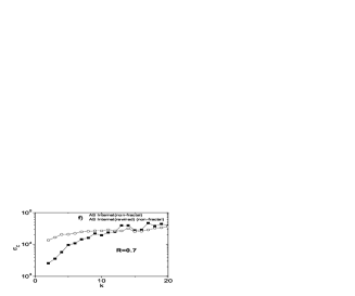
Figure 2: Betweenness centrality variance $\sigma_{C}$ calculated for both original and rewired networks as a function of node degree $k$. Every point of the plot corresponds to the betweenness centrality variance calculated for nodes of the same degree $k$ and normalized over the corresponding average betweenness centrality value $<C>$ of the original network. Each of the plots includes the value of the betweenness centrality- degree correlation dispersion coefficient $R$, see Eq.(3). Note, that small degree nodes of fractal networks: fractal model 3f(a), yeast(c) and Uni Western Sydney WWW(e) have significantly larger variance of betweenness centrality compared to their randomly rewired counterparts which are non-fractals. On the other hand, small degree nodes of the non-fractal networks: non-fractal model 3nf(b), pharmaceutical(d) and AS internet(f) have betweenness centrality variance comparable or even smaller than that of their randomly rewired counterparts. As a result $R>1$ for fractal networks and $R<1$ or $R\approx 1$ for nonfractal networks. Thus, betweenness centrality - degree correlation is weaker in fractal networks than in non-fractals.

The quantitative description of the betweenness centrality - degree correlation can be given by the analysis of the betweenness centrality variance $\sigma_{C}(k)$ attributed to nodes of specific degree $k$. Larger values of the variance $\sigma_{C}(k)$ mean weaker correlations between degree and betweenness centrality of a node since nodes of the same degree have larger variations in betweenness centrality values. As seen in Fig. 2, in a region of small degree, betweenness centrality variance $\sigma_{C}(k)$ of fractal networks is significantly bigger than that of their respective randomly rewired counterparts which are not fractals. At the same time betweenness centrality variance of non-fractal networks is comparable or even smaller than that of the corresponding randomly rewired networks. Thus, the betweenness centrality of nodes of fractal networks is significantly less correlated with degree than in non-fractal networks.

This can be understood as a result of the repulsion between hubs found in fractals repulsion : large degree nodes prefer to connect to nodes of small degree and not to each other. Therefore, the shortest path between two nodes must necessarily pass small degree nodes which are found at all scales of a network. Thus, in fractal networks small degree nodes have a broad range of values of betweenness centrality while in non-fractal networks nodes of small degree generally have small betweenness centrality. Betweenness centralities of small degree nodes in fractal networks significantly decrease after random rewiring since the rewired network is no longer fractal. On the other hand, centralities of nodes in non-fractal networks either do not change or increase after rewiring of edges.

As seen in Fig.1(b), the main difference in the betweenness centrality - degree correlation between fractal and non-fractal SF networks reveals itself in the dispersion of betweenness centrality values attributed to nodes of given degree, rather than in the average betweenness centrality values. So, in order to characterize and quantify the overall betweenness centrality - degree correlation we propose a correlation dispersion coefficient:

$$R=\frac{\sum_{k}\sigma_{C}(k)*p(k)}{\sum_{k}\sigma^{*}_{C}(k)*p(k)},$$ (3)

where $\sigma_{C}(k)$ and $\sigma^{*}_{C}(k)$ are the betweenness centrality variances of the original and randomly rewired networks respectively and $p(k)$ is the degree distribution of both networks. The dispersion coefficient $R$ is the ratio between the mean variance $<\sigma_{C}(k)>$ of the original network and $<\sigma^{*}_{C}(k)>$, the mean variance of the randomly rewired network. We note that fractal SF networks have bigger values of the betweenness centrality variance than their randomly rewired counterparts and therefore, have correlation dispersion coefficient $R>1$. On the other hand $\sigma_{C}(k)$ of the non-fractal SF networks is close or smaller than that of their random counterparts $\sigma^{*}_{C}(k)$ which result in values of the correlation dispersion coefficient $R\approx 1$ or $R<1$. The calculated values of the correlation dispersion coefficient $R$ for the networks we considered in the paper are summarized in Table. I.

The probability density function (pdf) of betweenness centrality has been studied for both Erdös Rényi ER ; ER_random graphs and SF scaling_in_nw networks. It was found that for SF networks the betweenness centrality distribution satisfies a power law

$$P(C)\sim C^{-\delta},$$ (4)

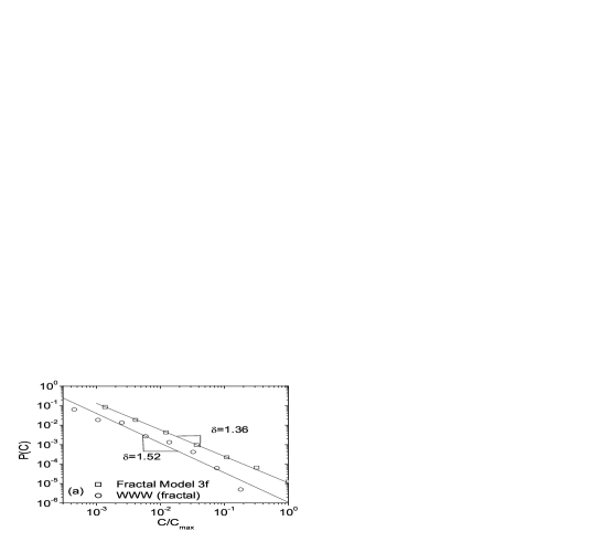
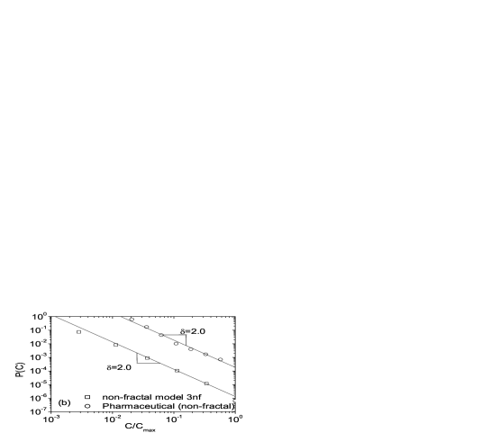
Figure 3: Betweenness centrality distributions of (a) Fractal model 3f and WWW network (fractal) and (b) non-fractal model 3nf and pharmaceutical network (non-fractal). The data have been binned logarithmically. Both fractal and non-fractal networks exhibit a power-law range of betweenness centrality distribution consistent with $P(C)\sim C^{-\delta}$. The measured betweenness centrality distributions (data points) are in good agreement with analytically obtained formula $\delta=2-1/d_{B}$ represented by the straight lines. In non-fractal networks we expect $\delta\rightarrow 2$ since $d_{B}\rightarrow\infty$.

with typical values of $\delta$ between 1 and 2 centr_distr_1 ; centr_distr_2 ; Braunstein_review . Our studies of the betweenness centrality distribution support these earlier results (Fig. 3). We find that $\delta$ increases with dimension $d_{B}$ of analyzed fractal networks. In the case of non-fractal networks, where $d_{B}=\infty$, estimated values of $\delta$ seem to be close to $2$.

An analytic expression for $\delta$ can be derived for SF fractal tree networks by using arguments similar to those used in Braunstein_review to find $\delta$ for the minimum spanning tree (MST). Consider a fractal tree network of dimension $d_{B}$. A small region of the network consisting of $n$ nodes will have a typical diameter $\ell(n)\sim n^{1/d_{B}}$ Bunde_Havlin . Nodes in this region will be connected to the rest of the network via $\ell(n)$ nodes. Thus, the betweenness centrality of those nodes is at least $n$. Since the number of regions of size $n$ is $N/n$, the total number of nodes with betweenness centrality $C>n$ in the network is

$$\phi(C>n)\sim\ell(n){N\over n}\sim n^{1/d_{B}-1}.$$ (5)

Thus, the number of links with betweenness centrality $n$ is

$$P(C)=\Delta\phi\sim\phi(C+1)-\phi(C)\sim C^{1/d_{B}-2}.$$ (6)

Using Eq. (4) we immediately obtain

$$\delta=2-{1\over d_{B}}.$$ (7)

Thus, Eq. (7) shows that $\delta$ increases with $d_{B}$ in agreement with Fig. 3. For non-fractal networks $d_{B}\rightarrow\infty$ and $\delta=2$. So non-fractal networks consist of relatively small number of central nodes and a large number of leaves connected to them. On the other hand in fractal networks, especially in those of small dimensionality, due to the repulsion between hubs, betweenness centrality is distributed among all nodes of a network. Analysis of the box covering method as a fractal test for some fractal and non-fractal networks studied here is shown in Fig. 4.

III Crossover scaling in fractal networks

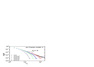
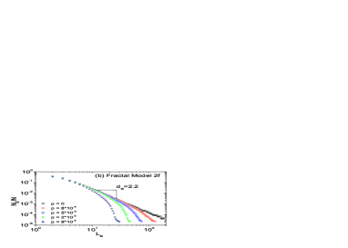
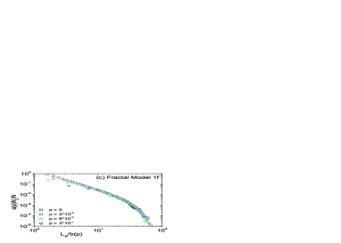
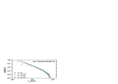
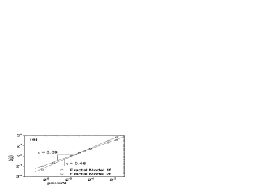
Figure 5: (a,b) Box-covering analysis of fractal models 1f and 2f with added random edges. Networks remain fractal for length scales smaller than certain crossover length $\ell^{*}$. Above $\ell^{*}$ the networks are no longer fractals. The crossover length $\ell^{*}$ becomes smaller as we add more edges. (c,d) Data collapse of $N_{B}(\ell,p)$ for the two fractal models. Appropriate rescaling $N_{B}(\ell_{B})\longrightarrow a(p)N_{B}(\ell_{B}/b(p))$ allows to collapse all the values of $N_{B}(l,p)$ onto a single curve. (e) The rescaling function $b(p)\equiv\ell^{*}$ for fractal models 1f and 2f as a function of $p$ shows a power law scaling of the crossover length $\ell^{*}\sim p^{-\tau}$. Calculated exponents are $\tau_{1}=0.46$ and $\tau_{2}=0.39$ respectively. Calculated values are slightly smaller than the expected values due to finite size effects.

We now study the behavior of fractal and non-fractal networks upon adding random edges. We analyze the crossover from fractal to non-fractal structure when random edges are added. To this end, we study the minimal number of boxes $N_{B}$ of size $\ell_{B}$ needed to cover the network as a function of $\ell_{B}$ as we add random edges to the network. Fig. 5(a) and  5(b) show that the dimension $d_{B}$ of the networks does not change. However, the network remains fractal with a power law regime $N_{B}\sim\ell^{-d_{B}}$ only at length scales $\ell$ below $\ell^{*}$, a characteristic length which depends on $p$. For $\ell>\ell^{*}$, the network with added random edges behaves as non-fractal with exponential decay $N_{B}\sim\exp(-\ell/\ell^{*})$. The crossover length $\ell^{*}$ separating the fractal and non-fractal regions decreases as we add more edges [see Figs. 5(a) and 5(b)]. We employ a scaling approach to deduce the functional dependence of the crossover length on the density of added shortcuts $p$. We propose for $N_{B}$ the scaling ansatz

$$N_{B}(\ell,p)\sim\ell^{*}(p)^{-d_{B}}F({\ell\over\ell^{*}(p)}),$$ (8)

where

$$F(u)\sim\left\{\begin{array}[]{ll}u^{-d_{B}}&~{}~{}~{}u\ll 1\\ \exp(-u)&~{}~{}~{}u\gg 1.\end{array}\right.$$ (11)

With appropriate rescaling we can collapse all the values of $N_{B}(\ell,p)$ onto a single curve [see Figs. 5(c) and 5(d)]. The crossover length $\ell^{*}(p)$ exhibits a clear power law dependence on the density of random shortcuts [Fig. 5(e)],

$$\ell^{*}(p)\sim p^{-\tau}.$$ (12)

We next argue that asymptotically for large $N$,

$$\tau=1/d_{B}.$$ (13)

When a fractal network with $N$ nodes and $E$ edges has additional $\Delta\ll N$ random edges, the probability of a given node $i$ to have a random link is $P_{i}=2\Delta/N$. The mass of the cluster within a size $\ell$ in a fractal network is $M_{C}\sim\ell^{d_{f}}$. The probability of $M_{C}(\ell)$ possessing a random edge is $P=(2\Delta/N)M_{C}$. Thus, at distances $\ell$ for which $(2\Delta/N)M_{C}\ll 1$ we are in the fractal regime. On the other hand, large distances $\ell$ for which $(2\Delta/N)M_{C}\gg 1$ correspond to the non-fractal regime. Thus, the crossover length $\ell^{*}$ corresponds to $(2\Delta/N)M_{C}(\ell^{*})\sim 1$, which implies $\ell^{*}\sim\Delta^{-1/d_{B}}$ or $\ell^{*}\sim p^{-1/d_{B}}$, where $p\equiv\Delta/N$. Note that the values measured for the two fractal networks, shown in Fig. 5(e), $\tau=0.46$ $(d_{B}=1.9)$ and $\tau=0.39$ $(d_{B}=2.3)$, are slightly smaller then the expected asymptotic values, which we attribute as likely to be due to finite size effects.

IV Discussion and Summary

We have shown that node betweenness centrality and node degree are significantly less correlated in fractal SF networks compared to non-fractal SF networks due to the effect of repulsion between the hubs. Betweenness centrality distribution in SF networks obeys a power law $P(C)\sim C^{-\delta}$. We derived an analytic expression for the betweenness centrality distribution exponent $\delta=2-1/d_{B}$ for SF fractal trees. Hence, fractal networks with smaller dimension $d_{B}$ have more nodes with higher betweenness centrality compared to networks with larger $d_{B}$. The transition from fractal to non-fractal behavior was studied by adding random edges to the fractal network. We observed a crossover from fractal to non-fractal regimes at a crossover length $\ell^{*}$. We found both analytically and numerically that $\ell^{*}$ scales with density of random edges $p$ as $\ell^{*}\sim p^{-\tau}$ with $\tau=1/d_{B}$.

V Acknowledgements

We thank ONR, European NEST, project DYSONET and Israel Foundation of Science for financial support. We are grateful to M. Riccaboni, O. Penner, and S. Sreenivasan for helpful discussions.

Appendix A A fractal growth model

A growth model of fractal SF networks was first introduced by Song et al. repulsion . In the core of the growth model lies the network renormalization technique self-sim ; repulsion : A network is covered with $N_{B}$ boxes of size $\ell_{B}$. Subsequently, each of the boxes is replaced by a node to construct the renormalized network. The process is repeated until the network is reduced to a single node. The fractal growth model represents the inverse of this renormalization process. The growth process is controlled by three parameters: $n$, $m$ and $e$ so that:

$$N(t) = n*N(t-1)$$ (14)

$$k_{i}(t) = m*k_{i}(t-1),$$ (15)

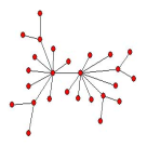
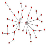
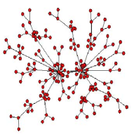
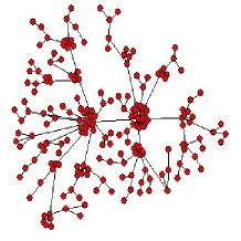
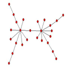
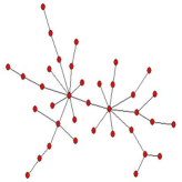
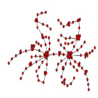
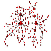
Figure 6: Constructing (a) non-fractal and (b) fractal networks with parameters $n=6$, $m=3$. The key difference between a fractal and non-fractal model is “repulsion between hubs”. In fractal networks nodes of large degree prefer to connect to nodes of small degree and not to nodes of large degree.

where $N(t)$ and $k_{i}(t)$ are, respectively, the number of nodes of the network and degree of node $i$ at time $t$. The parameter $e$ is the probability of hub attraction $e\equiv E_{\rm hubs}/E$. In the present study we limit our consideration to two distinct types of models: fractal ($e=0$) and non-fractal ($e=1$). At each growth step we run through all existing nodes. With probability $e$ we increase the degree of a given node by attaching $(m-1)k_{i}(t-1)$ new nodes (this corresponds to hub attraction). With probability $1-e$ we grow $(m-1)k_{i}(t-1)-1$ nodes using remaining node to repel hubs. Thus, the entire growth process can be summarized as follows (see Fig. 6):

• Start with a single node

• Connect $(m-1)k_{i}(t-1)$ extra nodes to each node $i$ to satisfy Eq. (15). With probability $1-e$ use one of the new nodes to repel node $i$ from the central node.

• Attach the remaining number of nodes to the network randomly to satisfy Eq. (14).

• Repeat steps (2) and (3) for the desired number of generations $g$.

The networks constructed in this way are SF with

$$\lambda=1+{\log n\over\log m}.$$ (16)

Fractal networks have a finite dimension

$$d_{B}={\log n\over\log 2}.$$ (17)

For derivations of Eqs. (16) and (17) see Ref. repulsion .

Here we refer to network models using a set of numbers (g,n,m,e). For example, the set $(4,5,3,0)$ should read as a 4th generation ($g=4$) fractal ($e=0$) network with $n=5$ and $m=3$. According to the above growth process for this example, $(4,5,3,0)$, $N=n^{g}=625$, $E=N-1=624$, $\lambda=1+\log n/\log m=2.46$, and $d_{B}=\log n/\log 2=2.32$.

Appendix B Modified box counting method.

The box counting method is used to calculate the minimum number of boxes $N_{B}$ of size $\ell_{B}$ needed to cover the entire network of $N$ nodes. The size of the box, $\ell_{B}$, imposes a constraint on the number of nodes that can be covered: all nodes covered by the same box must be connected and the shortest path between any pair of nodes in the box should not exceed $\ell_{B}$. The most crucial and time-consuming part of the method is to find the minimum out of all possible combinations of boxes. In the present study we use an approximate method that allows to estimate the number of boxes rather fast.

• Choose a random node (seed) on the network.

• Mark a cluster of radius $\ell_{B}$ centered on the chosen node.

• Choose another seed on the unmarked part of the network.

• Repeat steps (2) and (3) until the entire network is covered. The total number of seeds $N^{\prime}$ is an estimate of the required number of boxes $N_{B}$.

We stress that the estimated number of clusters $N^{\prime}$ is always less than $N_{B}$, the minimal number of boxes needed to cover the entire network. Indeed, the shortest path between any two seeds is greater then the size of the box $\ell_{B}$. Thus, a box cannot contain more than one seed, and in order to cover the whole network we need at least $N^{\prime}$ boxes.

Even though $N^{\prime}$ is always less or equal to $N_{B}$, the estimate may be good or poor based on the order we choose for the nodes. In order to improve the estimation we compute many times $N^{\prime}$ (typically 100–1000) and choose the maximum of all $N^{\prime}$.

Figures 4(a) and 4(b) demonstrate the application of the modified box counting algorithm to several fractal and non-fractal networks. According to Eq. (1), dimensions of the fractal networks are obtained by calculating the slope of the $N_{B}(\ell_{B})$ function in log-log format. The calculated dimensions are slightly underestimated due to a finite size effect of the analyzed networks.

Figure 4(c) represents $d_{B}$ as a function of the inverse number of generations $g$ of the model. As number of generations $g$ increases calculated dimension $d_{B}$ approaches the value given by Eq. (17).

A similar algorithm was introduced in Ref. crit_and_supercrit_skelet . The authors of this algorithm argue that it provides the same dimension of the network no matter how the boxes are chosen. In our algorithm we intend to estimate not only the dimension of the network but also the number of boxes. Thus, we are seeking the maximum $N^{\prime}$ out of many realizations.

Network Name	N	E	$\lambda$	$d_{B}$	Category
Model 1nf(7,4,2,1)	16384	16383	3.0	N/A	Non-Fractal
Model 2nf(6,6,2,1)	46656	46655	3.6	N/A	Non-Fractal
Model 3nf(8,3,2,1)	6561	6560	2.6	N/A	Non-Fractal
Model 1f(7,4,2,0)	16384	16383	3.0	2.	Fractal
Model 2f(6,6,2,0)	46656	46655	3.6	2.6	Fractal
Model 3f(8,3,2,0)	6561	6560	2.6	1.6	Fractal
SF Model	2668	3875	2.5	N/A	Non-Fractal
Uni West Sydney WWW	2526	4097	2.2	2.1	Fractal
Pharmaceutical  Pharm	6776	19801	2.4	N/A	Non-Fractal
Yeast  Barabasi	1458	1948	2.4	4.2	Fractal
AS Internet  dimes	20556	62920	2.1	N/A	Non-Fractal

Table 1: Properties of the networks studied in the paper. Here $N$ is the number of nodes, $E$ the number of edges, $\lambda$ the degree distribution exponent ($P(k)\sim k^{-\lambda}$) and $d_{B}$ is the fractal dimension. The notation of model networks is explained in Appendix A. We consider only the largest connected cluster of the network if the original network is disconnected.

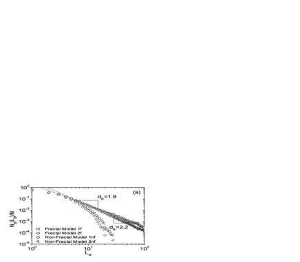
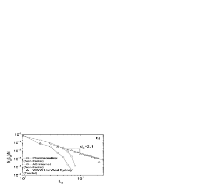
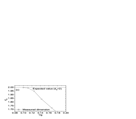
Figure 4: Box-covering method applied to (a) models: 1f, 2f, 1nf and 2nf and (b) real networks: WWW, Pharmaceutical, and AS Internet. The log-log plots of the number of boxes $N_{B}$ needed to cover the network as a function of their size $l_{B}$ show clear “power-law” behavior for the fractal networks. The calculated dimensions are presented in Table I. (c) The calculated dimension of fractal model 1f for different generations $g$ of the same fractal model network. Calculated value of $d_{B}$ approaches the expected value ($d_{B}=2$) as the number of generations increases.

References

- (1) R. Albert and A.-L. Barabási Rev. Mod. Phys. 74, 47 (2002).
- (2) S. N. Dorogovtsev and J. F. F. Mendes, Evolution of Networks: From Biological Nets to the Internet and WWW (Oxford University Press, Oxford, 2003).
- (3) R. Pastor-Satorras and A. Vespignani, Evolution and Structure of the Internet: A Statistical Physics Approach (Cambridge University Press, Cambridge, 2004).
- (4) R. Cohen and S. Havlin (Cambridge University Press, Cambridge,in press 2007).
- (5) P. Erdös and A. Rényi, Publ. Math. Inst. Hung. Acad. Sci. 6, 290 (1959).
- (6) P. Erdös and A. Rényi, Publ. Math. Inst. Hung. Acad. Sci. 5, 17 (1960).
- (7) B. Bollobas, Random Graphs (Cambridge University Press, 2001).
- (8) S. Milgram, Psychol. Today 2, 60 (1967).
- (9) D. J. Watts and S. H. Strogatz, Nature 393, 440 (1998).
- (10) R. Albert, H. Jeong, and A.-L. Barabasi, Nature 401, 130 (1999).
- (11) A. L. Barabási and R. Albert, Science 286, 509 (1999).
- (12) M. Faloutsos, P. Faloutsos, and C. Faloutsos, Comput. Comm. Rev. 29, 251 (1999).
- (13) C. Song, S. Havlin, and H. Makse, Nature 433, 392 (2005).
- (14) C. Song, S. Havlin, and H. Makse, Nature Physics 2, 275 (2006).
- (15) K. I. Goh, G. Salvi, B. Kahng, and D. Kim, Phys. Rev. Lett. 96, 018701 (2006).
- (16) J. S. Kim, K. I. Goh, G. Salvi, E. Oh, B. Kahng, and D. Kim, cond-mat/0605324.
- (17) S.-H. Yook, F. Radicci and H. Meyer-Ortmanns, Phys. Rev. E. 72, 045105(R) (2005).
- (18) J. Feder, Fractals (Plenum, New York, 1988).
- (19) M.E.J. Newman, Phys. Rev. Lett. 89, 208701 (2002).
- (20) L. C. Freeman, Social Networks 1, 215 (1979).
- (21) S. Wasserman and K. Faust, Social Network Analysis (Cambridge University Press, Cambridge, 1994)
- (22) J. Scott, Social Network Analysis: A Handbook (Sage Publications, London, 2000)
- (23) M. E. J. Newman, Phys. Rev. E. 64, 016132 (2001).
- (24) Z. Wu, L. A. Braunstein, S. Havlin and H. E. Stanley, Phys. Rev. Lett. 96, 148702 (2006).
- (25) L. Orsenigo, F. Pammolli, and M. Riccaboni, Research Policy, 30(3), 485 (2001).
- (26) http://netdimes.org (The DIMES project).
- (27) S. Carmi, S. Havlin, S. Kirkpatrick, Y. Shavitt and E. Shir, cs.NI/0607080 (2006).
- (28) http://www.nd.edu/alb/ (Home page of A. L. Barabási).
- (29) H. Jeong, S. Mason, A.-L. Barabási), Z.N.Oltvai, Nature 411, 41 (2001).
- (30) http://cybermetrics.wlv.ac.uk/database/ (The Academic Web Link Database Project).
- (31) P. Holme, B. J. Kim, C. N. Yoon, and S. K. Han, Phys. Rev. E 65, 056109 (2002).
- (32) D. H. Kim, J.D. Noh, and H. Jeong, Phys. Rev. E 70, 046126 (2004).
- (33) K. I. Goh, J. D. Noh, B. Kahng, and D. Kim, Phys. Rev. E 72, 017102 (2005).
- (34) L. A. Braunstein, Z. Wu, T. Kalisky, Y. Chen, S. Sreenivasan, R. Cohen, E. López, S. V. Buldyrev, S. Havlin, and H. E. Stanley, “Optimal Path and Minimal Spanning Trees in Random Weighted Networks”, Journal of Bifurcation and Chaos xx, xxx–xxx (2006). cond-mat/0606338.
- (35) A. Bunde and S. Havlin, eds., Fractals in Science (Springer, Berlin, 1996).