Deterministic Modularity Optimization

Abstract

We study community structure of networks. We have developed a scheme for maximizing the modularity $Q$ newman:04a based on mean field methods. Further, we have defined a simple family of random networks with community structure; we understand the behavior of these networks analytically. Using these networks, we show how the mean field methods display better performance than previously known deterministic methods for optimization of $Q$.

I Introduction

A theoretical foundation for understanding complex networks has developed rapidly over the course of the past few years albert:02 ; dorogovtsev:02 ; newman:03a . More recently, the subject of detecting network communities has gained an large amount of attention, for reviews see Refs newman:04d ; danon:05a . Community structure describes the property of many networks that nodes divide into modules with dense connections between the members of each module and sparser connections between modules.

In spite of a tremendous research effort, the mathematical tools developed to describe the structure of large complex networks are continuously being refined and redefined. Essential features related to network structure and topology are not necessarily captured by traditional global features such as the average degree, degree distribution, average path length, clustering coefficient, etc. In order to understand complex networks, we need to develop new measures that capture these structural properties. Understanding community structures is an important step towards developing a range of tools that can provide a deeper and more systematic understanding of complex networks. One important reason is that modules in networks can show quite heterogenic behavior newman:06b , that is, the link structure of modules can vary significantly from module to module. For such heterogenic systems, global measures can be directly misleading. Also, in practical applications of network theory, knowledge of the community structure of a given network is important. Access to the modular structure of the internet could help search engines supply more relevant responses to queries on terms that belong to several distinct communities. In biological networks, modules can correspond to functional units of some biological system barabasi:04 .

II The Modularity

This section is devoted to an analysis of the modularity $Q$. Identifying communities in a graph has a long history in mathematics and computer science chung:97 ; newman:04d . One obvious way to partition a graph into $C$ communities is distribute nodes into the communities, such that the number of links connecting the different modules of the network is minimized. The minimal number of connecting links is called the cut size $R$ of the network.

Consider an unweighted and undirected graph with $n$ nodes and $m$ links. This network can be represented by an adjacency matrix $\mathbf{A}$ with elements

$$A_{ij}=\left\{\begin{array}[]{ll}1,&\hbox{if there is a link joining nodes $i$ and $j$;}\\ 0&\hbox{otherwise.}\end{array}\right.$$ (1)

This matrix is symmetric with $2m$ entries. The degree $k_{i}$ of node $i$ is given by $k_{i}=\sum_{j}A_{ij}$. Let us express the cut-size in terms of $\mathbf{A}$; we find that

$$R=\frac{1}{2}\sum_{i,j}A_{ij}[1-\delta(c_{i},c_{j})],$$ (2)

where $c_{i}$ is the community to which node $i$ belongs and $\delta(\alpha,\beta)=1$ if $\alpha=\beta$ and $\delta(\alpha,\beta)=0$ if $\alpha\neq\beta$. Minimizing $R$ is an integer programming problem that can be solved exactly in polynomial time goldschmidt:88 . The leading order of the polynomial, however, is $n^{C^{2}}$ which very expensive for even very small networks. Due to this fact, most graph partitioning has been based on spectral methods (more below).

Newman has argued newman:04d ; newman:06a ; newman:06b that $R$ is not the right quantity to minimize in the context of complex networks. There are several reasons for this: First of all, the notion of cut-size does not capture the essence of our ‘definition’ of network as a tendency for nodes to divide into modules with dense connections between the members of module and sparser connections between modules. According to Newman, a good division is not necessarily one, in which there are few edges between the modules, it is one where there are fewer edges than expected. There are other problems with $R$: If we set the community sizes free, minimizing $R$ will tend to favor small communities, thus the use of $R$ forces us to decide on and set the sizes of the communities in advance.

As a solution to these problems, Girvan and Newman propose the modularity $Q$ of a network newman:04a , defined as

$$Q=\frac{1}{2m}\sum_{ij}[A_{ij}-P_{ij}]\delta(c_{i},c_{j}).$$ (3)

The $P_{ij}$, here, are a null model, designed to encapsulate the ‘more edges than expected’ part of the intuitive network definition. It denotes the probability that a link exists between node $i$ and $j$. Thus, if we know nothing about the graph, an obvious choice would be to set $P_{ij}=p$, where $p$ is some constant probability. However, we know that the degree distributions of real networks are often far from random, therefore the choice of $P_{ij}\sim k_{i}k_{j}$ is sensible; this model implies that the probability of a link existing between two nodes is proportional to the degree of the two nodes in question. We will make exclusive use of this null model in the following; the properly normalized version is $P_{ij}=(k_{i}k_{j})/(2m)$. It is axiomatically demanded that that $Q=0$ when all nodes are placed in one single community. This constrains the $P_{ij}$ such that

$$\sum_{ij}P_{ij}=2m,$$ (4)

we also note that $\mathbf{P}=(\mathbf{P})^{T}$, which follows from the symmetry of $\mathbf{A}$.

Comparing Eqs. (2) and (3), we notice that there are two differences between $Q$ and $R$. The first is that $Q$ implies that we maximize the number of intra-community links instead of minimizing the the number of inter-community links as is the case for $R$—this is the difference between multiplying by $\delta(c_{i},c_{j})$ and $[1-\delta(c_{i},c_{j})]$. The second difference lies in the the introduction of the $P_{ij}$ in Equation (3). The subtraction of $P_{ij}$ serves to incorporate information about the inter-community links into the quantity we are optimizing.

Use of modularity to identify network communities is not, however, completely unproblematic. Criticism has been raised by Fortunato and Barthélemy fortunato:06 who point out that the $Q$ measure has a resolution limit. This stems from the fact that the null model $P_{ij}\sim k_{i}k_{j}$ can be misleading. In a large network, the expected number of links between two small modules is small and thus, a single link between two such modules is enough to join them into a single community. A variation of the same criticism has been raised by Rosvall and Bergstrom rosvall:06a . These authors point out that the normalization of $P_{ij}$ by the total number of links $m$ has the effect that if one adds a distinct (not connected to the remaining network) module to the network being analyzed and partition the whole network again allowing for an additional module, the division of the original modules can shift substantially due to the increase of $m$.

In spite of these problems, the modularity is a highly interesting method for detecting communities in complex networks when we keep in mind the limitations pointed out above. What makes the modularity particularly interesting compared to other clustering methods is its ability to inform us of the optimal number of communities for a given network.

III Spectral Optimization of Modularity

The question of finding the optimal $Q$ is a discrete optimization problem. We can estimate the size of the space we must search to find the maximum. The number of ways to divide $n$ vertices into $C$ non-empty sets (communities) is given by the Stirling number of the second kind $S_{n}^{(C)}$ mathworld . Since we do not know the number of communities that will maximize $Q$ before we begin dividing the network, we need to examine a total of $\sum_{C=2}^{n}S_{n}^{(C)}$ community divisions newman:04b . Even for small networks, this is an enormous space, which renders exhaustive search out of the question.

Motivated by the success of spectral methods in graph partitioning, Newman suggests a spectral optimization of $Q$ newman:06a . We define a matrix, called the modularity matrix $\mathbf{B}=\mathbf{A}-\mathbf{P}$ and an $(n\times C)$ community matrix $\mathbf{S}$. Each column of $\mathbf{S}$ corresponds to a community of the graph and each row corresponds to a node, such that the elements

$$S_{ic}=\left\{\begin{array}[]{ll}1,&\hbox{if node $i$ belongs to community $c$;}\\ 0&\hbox{otherwise.}\end{array}\right.$$ (5)

Since each node can only belong to one community, the columns of $\mathbf{S}$ are orthogonal and $\mathrm{Tr}(\mathbf{S}^{T}\mathbf{S})=n$. The $\delta$-symbol in Equation (3) can be expressed as

$$\delta(c_{i},c_{j})=\sum_{k=1}^{C}S_{ik}S_{jk},$$ (6)

which allows us to express the modularity compactly as

$$Q=\frac{1}{2m}\sum_{i,j=1}^{n}\sum_{k=1}^{C}B_{ij}S_{ik}S_{jk}=\frac{\mathrm{Tr}(\mathbf{S}^{T}\mathbf{B}\mathbf{S})}{2m}.$$ (7)

This is the quantity that we wish to maximize.

The next step is the ‘spectral relaxation’, where we relax the discreteness constraints on $\mathbf{S}$, allowing elements of this matrix to possess real values. We do, however, constrain the length of the column vectors by $\mathbf{S}^{T}\mathbf{S}=\mathbf{M}$, where $\mathbf{M}$ is a $C\times C$ matrix with the number of nodes in each community $n_{1},n_{2},\ldots,n_{C}$ along the diagonal. In order to determine the maximum, we take

$$\frac{\partial}{\partial\mathbf{S}}\left(\frac{1}{2m}\mathrm{Tr}[\mathbf{S}^{T}\mathbf{B}\mathbf{S}]+\mathrm{Tr}[(\mathbf{S}^{T}\mathbf{S}-\mathbf{M})\tilde{\Lambda}]\right)=0,$$ (8)

where $\tilde{\Lambda}$ is a $C\times C$ diagonal matrix of Lagrange multipliers. The maximum is given by

$$\mathbf{B}\mathbf{S}=\mathbf{S}\Lambda,$$ (9)

where $\Lambda=-2m\tilde{\Lambda}$ for cosmetical reasons. Eq. (9) is a standard matrix eigenvalue problem. Optimizing in the relaxed representation, we substitute this solution into Eq. (7), and see that in order to maximize $Q$, we must choose the $C$ largest eigenvalues of $\mathbf{B}$ and their corresponding eigenvectors. Since all rows and columns of $\mathbf{B}$ sum to zero by definition, the vector $(1,1,\ldots,1)^{T}$ is always an eigenvector of $\mathbf{B}$ with the eigenvalue $0$. In general the modularity matrix can have both positive and negative eigenvalues. It is clear from Eq. (7) that the eigenvectors corresponding to negative eigenvalues can never yield a positive contribution to the modularity. Thus, the number of positive eigenvalues presents an upper bound on the number of possible communities.

However, we need to convert our problem back to a discrete one. This is a non-trivial task. There is no standard way to go from the $n$ continuous entries in each of the $C$ largest eigenvectors of the modularity matrix and back to discrete $0,1$ values of the community matrix $\mathbf{S}$. One simple way of circumventing this problem is to use repeated bisection of the network. This is the procedure that Newman newman:06a recommends. In Newman’s scheme, the only eigenvector utilized is the eigenvector corresponding to the largest eigenvalue $b_{\rm max}$ of $\mathbf{B}$ (with highest contribution to $Q$). The $0,1$ vector most parallel to this continuous eigenvector, is one where the positive elements of the eigenvector are set to one and the negative elements zero. This is the first column of the community matrix $\mathbf{S}$. The second column must contain the remaining elements.

We can increase the modularity iteratively by bisecting the network into smaller and smaller pieces. However, this repeated bisection of the network is problematic. There is no guarantee that that the best division into three groups can be arrived at by finding by first determine the best division into two and then dividing one of those two again. It is straight forward to construct examples where a sub-optimal division into communities is obtained when using bisection newman:06b ; reichardt:06a .

Spectral optimization is not perfect—especially when only the eigenvector corresponding to $b_{\rm max}$ is employed. Therefore, Newman suggests that it should only be used as a starting point. In order to improve the modularity, Newman has devised an algorithm inspired by the classical Kernighan-Lin (KL) scheme kernighan:70 . The procedure is as follows: After each bisection of the network we go through the nodes and find the one that yields the highest increase in the modularity of the entire network (or smallest decrease if no increase is possible) if moved to the other module. This node is now moved to the other module and becomes inactive. The next step is to go through the remaining $n-1$ nodes and perform the same action. We continue like this until all nodes have been moved. Finally, we go through all the intermediate states and pick the one with the highest value of $Q$. This is the new starting division. We proceed iteratively from this configuration until no further improvement can be found. Let us call this optimization the ‘KLN-algorithm’.

In the spectral optimization, the computational bottleneck is the calculation of the leading eigenvector(s) of $\mathbf{B}$, which is non-sparse. Naively, we would expect this to scale like $O(n^{3})$. However, $\mathbf{B}$’s structure allows for a faster calculation. We can write the product of $\mathbf{B}$ and a vector $\mathbf{v}$ newman:06a as

$$\mathbf{B}\mathbf{v}=\mathbf{A}\mathbf{v}-\frac{\mathbf{k}(\mathbf{k}^{T}\mathbf{v})}{2m}.$$ (10)

This way we have a divided the multiplication into (i) sparse matrix product with the adjacency matrix that takes $O(m+n)$, and (ii) the inner product $\mathbf{k}^{T}\mathbf{v}$ that takes $O(n)$. Thus the entire product $\mathbf{B}\mathbf{v}$ scales like $O(m+n)$. The total running for a bisection determining the eigenvector(s) is therefore $O((m+n)n)$ rather than the naive guess of $O(n^{3})$. Using Eq. (10) during the KLN-algorithm reduces the cost of this step to $O((m+n)n)$ newman:06a .

IV Mean Field Optimization

Simulated annealing was proposed by Kirkpatrick et al. Kirkpatrick83 who noted the conceptual similarity between global optimization and finding the ground state of a physical system. Formally, simulated annealing maps the global optimization problem onto a physical system by identifying the cost function with the energy function and by considering this system to be in equilibrium with a heat bath of a given temperature $T$. By annealing, i.e., slowly lowering the temperature of the heat bath, the probability of the ground state of the physical system grows towards unity. This is contingent on whether or not the temperature can be decreased slowly enough such that the system stays in equilibrium, i.e., that the probability is Gibbsian

$$P(\mathbf{S}|T)=\frac{1}{Z}\exp\left(-\frac{1}{T}Q(\mathbf{S})\right)=\frac{1}{Z}\exp\left(-\frac{\mathrm{Tr}(\mathbf{S}^{T}\mathbf{B}\mathbf{S})}{2m}\right).$$ (11)

Here, $Z$ is a constant ensuring proper normalization. Kirkpatrick et al. realized the annealing process by Monte Carlo sampling. The representation of the constrained modularity optimization problem is equivalent to a $C$-state Potts model. Gibbs sampling for the Potts model with the modularity $Q$ as energy function has been investigated by Reichardt and Bornholdt, see e.g., reichardt:06a .

Mean field annealing is a deterministic alternative to Monte Carlo sampling for combinatorial optimization and has been pioneered by Peterson et al. Peterson87 ; Peterson89 . Mean field annealing avoids extensive stochastic simulation and equilibration, which makes the method particularly well suited for optimization. There is a close connection between Gibbs sampling and MF annealing. In Gibbs sampling, every variable is updated by random draw of a Potts state with a conditional distribution,

$$P(S_{i1},...,S_{iC}|\mathbf{S}_{\{-i\}},T)=\frac{P(\mathbf{S}|T)}{\sum_{S_{i1},...,S_{iC}}P(\mathbf{S}|T)},$$ (12)

where the sum runs over the $C$ values of the $i$’th Potts variable and $\mathbf{S}_{\{-i\}}$ denotes the set of Potts variables excluding the $i$’th node. As noted by reichardt:06a , Eq. (12) is local in the sense that the part of the energy function containing variables not connected with the $i$’th cancels out in the fraction. The mean field approximation is obtained by computing the conditional mean of the set of variables coding for the $i$’th Potts variable using Eq. (12) and approximating the Potts variables in the conditional probability by their means Peterson89 . This leads to a simple self-consistent set of non-linear equations for the means,

$$\mu_{ik}=\frac{\exp(\phi_{ik}/T)}{\sum_{k^{\prime}=1}^{C}\exp(\phi_{ik^{\prime}}/T)},\ \ \phi_{ik}=\sum_{j}B_{ij}\mu_{jk}.$$ (13)

For symmetric connectivity matrices with $\sum_{j}B_{ij}=0$, the set of mean field equations has the unique high-temperature solution $\mu_{ik}=1/C$. This solution becomes unstable at the mean field critical temperature, $T_{c}=b_{\rm max}/C$, determined by the maximal eigenvalue $b_{\rm max}$ of $\mathbf{B}$.

This mean field algorithm is fast. Each synchronous iteration (see Section VI for details on implementation) requires a multiplication of $\mathbf{B}$ by the mean vector $\mathbf{\mu}$. As we have seen, this operation can be performed in $O(m+n)$ time using the trick in Eq. (10). In these experiments, we have used a fixed number of iterations of the order of $O(n)$, which gives us a total of $O((m+n)n)$ similar to the case of by spectral optimization. (A forthcoming paper discusses the relationship between Gibbs sampling, mean field methods, and computational complexity.)

V A Simple Network

We will perform our numerical experiments on a simple model of networks with communities. This model network consists of $C$ communities with $n_{c}$ nodes in each, the total network has $n=n_{c}C$ nodes. Without loss of generality, we can arrange our nodes according to their community; a sketch of this type of network is displayed in Figure 1.

$$\begin{array}[]{cccccc}\framebox[28.45274pt][c]{\begin{minipage}[c]{28.45274pt} \begin{center}\vspace{.25cm} $p$ \vspace{.25cm} \end{center}\end{minipage}}&\framebox[28.45274pt][c]{\begin{minipage}[c]{28.45274pt} \begin{center}\vspace{.25cm} $q$ \vspace{.25cm} \end{center}\end{minipage}}&\cdots&\framebox[28.45274pt][c]{\begin{minipage}[c]{28.45274pt} \begin{center}\vspace{.25cm} $q$ \vspace{.25cm} \end{center}\end{minipage}}&$$\bigg{\}}n_{c}$$\\ \framebox[28.45274pt][c]{\begin{minipage}[c]{28.45274pt} \begin{center}\vspace{.25cm} $q$ \vspace{.25cm} \end{center}\end{minipage}}&\framebox[28.45274pt][c]{\begin{minipage}[c]{28.45274pt} \begin{center}\vspace{.25cm} $p$ \vspace{.25cm} \end{center}\end{minipage}}&&&\\ \vdots&&\ddots&&\\ \framebox[28.45274pt][c]{\begin{minipage}[c]{28.45274pt} \begin{center}\vspace{.25cm} $q$ \vspace{.25cm} \end{center}\end{minipage}}&&&\framebox[28.45274pt][c]{\begin{minipage}[c]{28.45274pt} \begin{center}\vspace{.25cm} $p$ \vspace{.25cm} \end{center}\end{minipage}}&\\ \lx@intercol\hfil\underbrace{\hskip 113.81102pt}_{n}\hfil\lx@intercol&\end{array}$$

Figure 1: A sketch of the simple network model. The figure displays the structure of the adjacency matrix with nodes arranged according to community. Inside each community (the blocks) along the diagonal, the probability of a link between two nodes is $p$ and between communities, the probability of a link is $q$.

Communities are defined as standard random networks, where the probability of a link between two nodes is given by $p$, with $0<p\leq 1$. Between the communities the probability of a link between is given by $0\leq q<p$. The networks are unweighted and undirected.

Let us calculate $Q$ for this network in the case where $p=1$ and $q=0$. In this case, we can calculate everything exactly. First, we note that all nodes have the same number of links, and that the degree of node $i$, $k_{i}=n_{c}-1$ (since a node does not link to itself). Thus the total number of links $m_{c}$ in each sub-network is

$$m_{c}=\frac{1}{2}n_{c}(n_{c}-1),$$ (14)

and since our network consists of $C$ identical communities the total number of links is $m=Cm_{c}$. We can now write down the contribution $Q_{c}$ from each sub-network to the total modularity

$$Q_{c} = \frac{1}{2m}\sum_{ij}(A_{ij}-P_{ij})\delta(c,c)$$ (15)

$$= \frac{1}{2m}\left[n_{c}(n_{c}-1)-n_{c}^{2}\frac{(n_{c}-1)^{2}}{2m}\right].$$ (16)

If we insert $m$ and use that $Q=CQ_{c}$, we find

$$Q=CQ_{c}=1-\frac{1}{C}.$$ (17)

We see explicitly that when $C\to\infty$ the modularity approaches unity.

Now, let us examine at the general case. Since our network is connected at random, we cannot calculate the number of links per node exactly, but we know that the network is well-behaved (Poisson link distribution), thus we can calculate the average number of links per node. We see that

$$k=(n_{c}-1)p+n_{c}(C-1)q,$$ (18)

which is equal to the number of expected intra-community links plus the number of expected number of inter-community links. The number of links in the entire network is therefore given by

$$m=\frac{1}{2}Cn_{c}k=\frac{Cn_{c}}{2}[(n_{c}-1)p+n_{c}(C-1)q].$$ (19)

We write down $Q$

$$Q = \frac{C}{2m}\left[n_{c}(n_{c}-1)p-n_{c}^{2}\frac{\{(n_{c}-1)p+n_{c}(C-1)q\}^{2}}{2m}\right]$$ (20)

$$= \frac{(n_{c}-1)p}{(n_{c}-1)p+n_{c}(C-1)q}-\frac{1}{C}.$$

When $n_{c}\gg 1$ (which is always the case), we have that

$$Q=\frac{p}{p+q(C-1)}-\frac{1}{C},$$ (21)

When we write $q$ as some fraction $f$ of $p$, that is $q=fp$, with $0\leq f\leq 1$, we find

$$Q(C,f)=\frac{1}{1+(C-1)f}-\frac{1}{C},$$ (22)

which is independent of $p$. Thus, for this simple network, the only two relevant parameters are the number of communities and the density of the inter-community links relative to the intra-community strength. We can also see that our result from Eq. (17) is valid even in the case $p<1$, as long as the communities are connected and $q=0$.

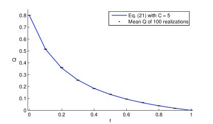
Figure 2: Equation (22) and $Q_{\text{design}}$. This figure displays $Q$ as a function of $f$ (the relative probability of a link between communities), with $C=5$ for the simple network defined in Figure 1. The blue line is given by Eq. (22) and the black dots with error-bars are mean values of $Q_{\text{design}}$ in realizations of the simple network with $p=1/10$ and $n=500$; each data-point is the mean of $100$ realizations. The error bars are calculated as the standard deviation divided by square root of the number of runs.

If we design an adjacency matrix according to Figure 1, we can calculate the value $Q_{\text{design}}=\mathrm{Tr}(\mathbf{S}_{\text{d}}^{T}\mathbf{B}\mathbf{S}_{\text{d}})/(2m)$, where $\mathbf{S}_{\text{d}}$ is a community-matrix that reflects the designed communities. Values of $Q_{\rm design}$ should correspond to Eq. (22). We see in Figure 2 that this expectation is indeed fulfilled. The blue curve is $Q$ as a function of $f$ with $C=5$. The black dots with error-bars are mean values of $Q_{\text{design}}$ in realizations of the simple network with $p=1/10$ and $n=500$; each data-point is the mean of $100$ realizations and the error bars are calculated as the standard deviation divided by square root of the number of runs. The correspondence between prediction and experiment is quite compelling.

We should note, however, that the value of $Q_{\rm design}$ may be lower than the actual modularity found for the network by a good algorithm: We can imagine that fluctuations of the inter-community links could result in configurations that would yield higher values of $Q$—especially for high values of $f$. We can quantify this quite precisely. Reichardt and Bornholdt reichardt:06a have shown that demonstrated that random networks can display significantly larger values of $Q$ due to fluctuations; when $f=1$, our simple network is precisely a random network (see also related work by Guimerà et al. guimera:04a ). In the case of the network we are experimenting on, ($n=500$, $p=1/10$), they predict $Q\approx 0.13$.

Thus, we expect that the curve for $Q(f,C)$ with fixed $C$ will be deviate from the $Q_{\text{design}}$ displayed in Figure 2; especially for values of $f$ that are close to unity. The line will decrease monotonically from $Q(0,C)=1-1/C$ towards $Q(1,C)=0.11$ with the difference becoming maximal as $f\to 1$.

VI Numerical Experiments

We know that the running time of mean field method scales like that of the spectral solution. In order to compare the precision of the mean field solutions to the solutions stemming from spectral optimization, we have created a number of test networks with adjacency matrices designed according to Figure 1. We have created $100$ test networks using parameters $n_{c}=100$, $C=5$, $p=0.1$ and $f\in[0,1]$. Varying $f$ over this interval allows us to interpolate between a model with $C$ disjunct communities and a random network with no community structure.

We applied the following three algorithms to our test networks

1. Spectral optimization,

2. Spectral optimization and the KLN-algorithm, and

3. Mean field optimization.

Spectral optimization and the KLN-algorithm were implemented as prescribed in newman:06a . The $nC$ non-linear mean field annealing equations were solved approximately using a $D=300$-step annealing schedule linear in $\beta=1/T$ starting at $\beta_{c}$ and ending in $3\beta_{c}$ at which temperature the majority of the mean field variables are saturated. The mean field critical temperature $T_{c}=b_{\rm max}/C$ is determined for each connectivity matrix. The synchronous update scheme defined as parallel update of all means at each of the $D$ temperatures

$$\mu_{ik}^{(d+1)} = \frac{\exp(\phi_{ik}^{(d)}/T)}{\sum_{k^{\prime}=1}^{C}\exp(\phi_{ik^{\prime}}^{(d)}/T)}$$

$$\phi_{ik}^{(d)} = \sum_{j}B_{ij}\mu_{jk}^{(d)}$$ (23)

can grow unstable at low temperatures. A slightly more effective and stable update scheme is obtained by selecting random fractions $\rho<1$ of the means for update in $1/\rho$ steps at each temperature. We use $\rho=0.2$ in the experiments reported below. A final $T=0$ iteration, equivalent to making a decision on the node community assignment, completes the procedure. We do not assume that actual the number of communities $C<C_{\rm max}$ is known in advance. In these experiments we use $C_{max}=8$. This number is determined after convergence by counting the number of non-empty communities

The results of the numerical runs are displayed in Figure 3. This figure shows the point-wise differences between the value of $Q_{\text{algorithm}}$ found by the algorithm in question and $Q_{\text{\rm design}}$ plotted as a function of the inter-community noise $f$.

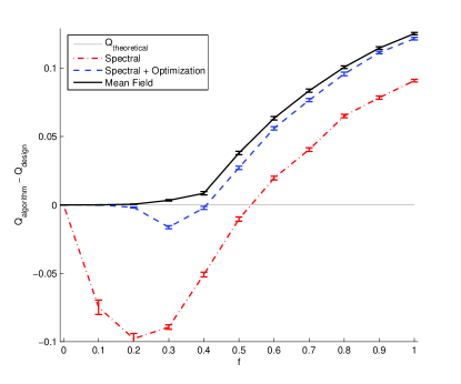
Figure 3: Comparing spectral methods with the mean field solution. The networks were created according to the simple model, using parameters $n_{c}=100$, $C=5$, $p=0.1$ and $f\in[0,1]$. All data points display the point-wise differences between the value of $Q_{\text{algorithm}}$ found by the algorithm in question and $Q_{\text{\rm design}}$. The error-bars are calculated as in Figure 2. The dash-dotted red line shows the results for the spectral method. The dashed blue line shows the results for the spectral optimization followed by KLN post-processing. The solid black curve shows the results for the mean field optimization. The grey, horizontal line corresponds to the theoretical prediction (Eq. (22)) for the designed communities.

The line of $Q_{\text{algorithm}}-Q_{\rm design}=0$ thus corresponds to the curve plotted in Figure 2. We see from Figure 3 that the mean field approach uniformly out-performs both spectral optimization and spectral optimization with KLN post-processing. We also ran a Gibbs sampler reichardt:06a for with a computational complexity equivalent to the mean field approach. This lead to communities with $Q$ slightly lower than the mean field results, but still better than spectral optimization with KLN post-processing.

We note that the obtained $Q_{\rm algorithm}$ for a random network ($f=1$) is consistent with the prediction made by Reichardt and Bornholdt reichardt:06a . We also see that the optimization algorithms can exploit random connections to find higher values of $Q_{\rm algorithm}$ than expected for the designed communities $Q_{\rm design}$. In the case of the mean field algorithm this effect is visible for values of $f$ as low as $0.2$.

Figure 4 shows the median number of communities found by the various algorithms as a function of $f$.

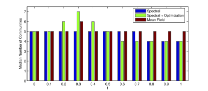
Figure 4: The median number of communities found by the various algorithms. The panel shows the median number of communities as a function of the relative fraction of inter-community links $f$. All optimization schemes consistently pick four or five communities for the highest values of $f$. This finding is consistent with theoretical and experimental results by Reichardt and Bornholdt reichardt:06a

It is evident from Figs. 3 and 4 that—for this particular set of parameters—the problem of detecting the designed community structure is especially difficult around $f=0.3$. Spectral clustering with and without the KLN algorithm find values $Q_{\rm algorithm}$ that are significantly lower than $Q_{\rm desigm}$. The mean field algorithm manages to find a value of $Q_{\rm algorithm}$ that is higher than the designed $Q$ but does so by creating extra communities. As $f\to 1$ it becomes more and more difficult to recover the designed number of communities.

VII Conclusions

We have introduced a deterministic mean field annealing approach to optimization of modularity $Q$. We have evaluated the performance of the new algorithm within a family of networks with variable levels of inter-community links, $f$. Even with a rather costly post-processing approach, the spectral clustering approach suggested by Newman is consistently out-performed by the mean field approach for higher noise levels. Spectral clustering without the KLN post-processing finds much lower values of $Q$ for all $f>0$.

Speed is not the only benefit of the mean field approach. Another advantage is that the implementation of mean field annealing is rather simple and similar to Gibbs sampling. This method also avoids the inherent problems of repeated bisection. The deterministic annealing scheme is directed towards locating optimal configurations without wasting time at careful thermal equilibration at higher temperatures. As we have noted above, the modularity measure $Q$ may need modification in specific non-generic networks. In that case, we note that the mean field method is quite general and can be generalized to many other measures.

References

- (1) M.E.J. Newman and M. Girvan. Finding and evaluating community structure in networks. Physical Review E, 69:026113, 2004, cond-mat/0308217.
- (2) R. Albert and A.-L. Barabási. Statistical mechanics of complex networks. Reviews of modern physics, 74:47, 2002.
- (3) S. N. Dorogovtsev and J. F. F. Mendes. Evolution of networks. Advances in Physics, 51:1079, 2002.
- (4) M. E. J. Newman. The structure and function of complex networks. SIAM Review, 45:167, 2003.
- (5) M.E.J. Newman. Detecting community structure in networks. The European Physical Journal B, 38:321, 2004.
- (6) L. Danon, J. Duch, A. Diaz-Guilera, and A. Arenas. Comparing community structure identification. Journal of Statistical Mechanics, page P09008, 2005, cond-mat/0505245.
- (7) M. E. J. Newman. Finding community structure in networks using the eigenvectors of matrices. Physical Review E, 74:036104, 2006.
- (8) A.-L. Barabási and Z. N. Oltvai. Network biology: Understanding the cell’s functional organization. Nature Reviews Genetics, 5:101, 2004.
- (9) F. K. R. Chung. Spectral Graph Theory. American Mathematical Society, 1997.
- (10) O. Goldscmidt and D. S. Hochbaum. Polynomial algorithm for the -cut problem. In Proceedings of the 29th Annual IEEE Symposium on the Foundations of Computer Science, page 444. Institute of Electrical and Electronics Engineers, 1988.
- (11) M. E. J. Newman. Modularity and community structure in networks. Proceedings of the National Academy of Sciences, USA, 103:8577, 2006.
- (12) S. Fortunato and M. Barthelemy. Resolution limit in community detection. Proceedings of the National Academy of Sciences USA, 104:36, 2007.
- (13) M. Rosvall and C. T. Bergstrom. An information-theoretic framework for resolving community structure in complex networks. 2006, physics/0612035.
- (14) Mathworld. http://mathworld.wolfram.com/.
- (15) M.E.J. Newman. Fast algorithm for detecting community structure in networks. Physical Review E, 69:066133, 2004, cond-mat/0309508.
- (16) J. Reichardt and S. Bornholdt. Statistical mechanics of community detection. Physical Review E, 74:016110, 2006.
- (17) B. M. Kernighan and S. Lin. An efficient heuristic procedure for partitioning graphs. The Bell System Technical Journal, 49:291, 1970.
- (18) S. Kirkpatrick, C.D. Gelatt Jr., , and M.P. Vecchi. Optimization by simulated annealing. Science, 220:671–680, 1983.
- (19) C. Peterson and J.R. Anderson. A mean field theory learning algorithm for neural networks. Complex Systems, 1:995–1019, 1987.
- (20) C. Peterson and B. Söderberg. A new method for mapping optimization problems onto neural networks. Int J Neural Syst, 1:3–22, 1989.
- (21) R. Guimerá, M. Sales-Pardo, and L. A. N. Amaral. Modularity from fluctuations in random graphs and complex networks. Physical Review E, 70:025101, 2004, cond-mat/0403660.